Merging History Trees of Dark Matter Haloes: a Tool for Exploring Galaxy Formation Models

Abstract

A method of deriving and using merging history trees of dark matter galaxy haloes directly from pure gravity N-body simulations is presented. This combines the full non-linearity of N-body simulations with the flexibility of the semi-analytical approach.

Merging history trees derived from power-law initial perturbation spectrum simulations (for indices $n=-2$ and $n=0$) by [Warren et al.] (1992) are shown. As an example of a galaxy formation model, these are combined with evolutionary stellar population synthesis, via simple scaling laws for star formation rates, showing that if most star formation occurs during merger-induced bursts, then a nearly flat faint-end slope of the galaxy luminosity function may be obtained in certain cases.

Interesting properties of hierarchical halo formation are noted: (1) In a given model, merger rates may vary widely between individual haloes, and typically 20%$\sim$30% of a halo’s mass may be due to infall of uncollapsed material. (2) Small mass haloes continue to form at recent times: as expected, the existence of young, low redshift, low metallicity galaxies (e.g., [Izotov et al.] 1997) is consistent with hierarchical galaxy formation models. (3) For $n=-2,$ the halo spatial correlation function can have a very high initial bias due to the high power on large scales.

1 Introduction

As quantitatively pioneered by those such as [Hoyle] (1953), [Silk] (1977) and [Rees & Ostriker] (1978) and more recently noted by authors such as Frenk et al. (1995), hierarchical galaxy formation models in $\Omega_{0}=1$ cold dark matter (CDM) universes typically combine assumptions on up to six distinct physical processes: (1) the non-linear growth phase of matter density peaks (known as “haloes”), (2) cooling gas dynamics, (3) star formation, (4) star-to-gas energy feedback, (5) stellar evolution, (6) galaxy mergers. In principle, if there are more free parameters describing these processes than independent observational galaxy statistics, then the observations should provide little constraint on galaxy formation “recipes”. Fortunately, the contrary is presently the case for the “semi-analytical ab initio” models which make various analytical estimates of process (1), combine semi-empirical and simple scaling parametrisations to represent processes (2)-(4) and (6) and use evolutionary stellar population synthesis for process (5). Since each of these models have problems explaining at least some of the observations means, the models are better constrained than might have been hoped for.

These models can be considered to be semi-analytical because rather than calculating what is possibly the most important process, the non-linear formation and merging history of collapsed objects [process (1)], via N-body simulations, various statistical analytical approximations are used. The models of Lacey et al. (1993) use an approximation developed in [Lacey & Silk] (1991) from the BBKS peaks formalism ([Bardeen et al.] 1986), Kauffmann et al. ([Kauffmann & White] 1993; [Kauffmann et al.] 1993) use a probabilistic method ([Bower] 1991) based on the Press-Schecter formalism (e.g., [Press & Schechter] 1974; White & Frenk 1991) and excursion set mass function calculations ([Bond et al.] 1991) while [Cole et al.] (1994) use a spatially quantised “block” method described in [Cole & Kaiser] (1988).

Further semi-analytical developments include those adding spatial auto-correlation information to a Press-Schechter formalism ([Mo & White] 1996) or to the “block” model ([Rodrigues & Thomas] 1996; [Nagashima & Gouda] 1997) and a technique of separately treating global, weakly non-linear and local, strongly non-linear dynamics (the “peak-patch” formalism, [Bond & Myers] 1996).

Each of the models which has been compared to observational statistics has difficulty in simultaneously explaining the flatness of the present-day (surface-brightness limited) galaxy luminosity function (e.g., Loveday et al. 1992), the steepness of the faint galaxy counts (e.g., [Tyson & Seitzer] 1988; [Tyson] 1988), the shape of the moderately faint galaxy ($B\,\lower 2.58334pt\hbox{$\buildrel<\over{\sim}$}\,23$) spectroscopic redshift distributions (e.g., [Colless et al.] 1990; [Colless et al.] 1993), the Tully-Fisher relation and the colour distributions of present-day galaxies, in a CDM $\Omega_{0}=1$ universe. Even though the [Cole et al.] (1994) model is better than the previous models in allowing big $z=0$ galaxies to be at least as red as higher $z$ galaxies, it shares the problem of the other models in lacking big red ellipticals. It also shares with the [Kauffmann et al.] model the problem that if the large number of small haloes predicted by CDM models at $z\approx 0$ follow the IR Tully-Fisher relation (e.g., [Pierce & Tully] 1992), then the slope of the faint end of the general galaxy luminosity function should be steeper than that estimated locally (e.g., Loveday et al. 1992). Changing the cosmology in the [Cole et al.] models ([Heyl et al.] 1995: low $H_{0}$, low $\Omega_{0}$, non-zero $\lambda_{0}$ and CHDM models) is insufficient to match the observations. Another way of allowing these models to fit the observations is to make a strong assumption for process (6)—to suppose that galaxies can merge as fast as galaxy haloes merge, or even faster—but simple present-day constraints on the products of the mergers ([Dalcanton] 1993) and the relative weakness of the faint galaxy angular auto-correlation function ([Roukema & Yoshii] 1993) strongly restrict this possibility.

In order to avoid problems which may be due to the approximation of non-linear gravitational collapse and evolution by the semi-analytical techniques mentioned above, an alternative technique is to calculate both processes (1) and (2) from first principles in numerical N-body simulations, folding in the other physical processes as simple scaling formulae or using stellar population synthesis for (5). Several authors (e.g., [Evrard] 1988; [Navarro & Benz] 1991; [Cen & Ostriker] 1992; [Umemura et al.] 1993; [Steinmetz & Müller] 1995) have experimented with these techniques, but resolution limits on present-day computers make the results hard to interpret. For example, [Weinberg et al.] (1997) point out that although low resolution gravito-hydrodynamic simulations suggest that a UV photoionisation background can suppress galaxy formation (by heating the gas so that it is unable to cool and form stars), higher resolution simulations show that this is a numerical artefact: the higher resolution simulations show little sensitivity to either the details of photoionisation or star formation.

In this article, rather than claiming a global “recipe” for galaxy formation, our primary purpose is to concentrate on process (1) in a way complementary to that of other techniques. This is unlikely to be sufficient to solve all the observational conflicts. On the contrary, this method should increase the ability of modellers to verify the extent to which model predictions are sensitive to the precision of modelling of gravity.

The method presented here is to derive merging history trees of dark matter haloes directly from N-body simulations. Rather than just investigating virialised haloes for a particular dark matter model (e.g., CDM), (a) both $n=-2$ and $n=0$ initial perturbation spectrum simulations (where $n$ is the index of the power spectrum) are examined, and (b) since the halo-to-galaxy relationship may be more complex than a simple one-to-one mapping, two significantly different density thresholds are used for halo detection. This reveals the sensitivity of halo merger history trees and halo statistics to these parameters. The N-body simulations used are presented in §2.1.1, the choice of a group-finding algorithm in §2.1.2 and the defining criterion and algorithm for calculating the merging history trees in §2.1.3.

Properties of the haloes detected are discussed in §2.2. In particular, the resulting merging history trees are presented in graphical form in §2.2.3, enabling patterns of halo merging calculated from fully non-linear simulations to be visualised directly.

If processes (2)-(5) are simple enough, and if process (6), galaxy merging, corresponds in a one-to-one way with halo merging, then these halo merger history trees would lead directly to galaxy merger history trees. We therefore examine an example application of the merger history trees by making minimal assumptions for processes (2)-(4), using stellar evolutionary population synthesis for process (5), and for process (6), assuming maximal galaxy merging (every halo merger corresponds to a galaxy merger). §3.1 presents (6)+(3) merger-induced star formation and §3.2 explains how process (5) is modelled.

In order for these processes to have an effect on the luminosity function, an option is considered in which each merger induces a burst of star formation, scaled according to the appropriate halo and gas masses and the dynamical time scale. Apart from this star formation rate option, we do not explore parameter space for non-gravitational processes in this paper; we merely adopt simple observationally normalised scaling laws. Resulting luminosity functions are presented in §3.3.

Applications of N-body derived halo merger trees with more complex assumptions for processes (2)-(6) are of course possible, and indeed to be welcomed. The galaxy formation “recipe” explored here is only one simple example.

Cosmological conventions adopted for this paper are a Hubble constant of $H_{0}=50\,$km s^-1Mpc^-1, comoving units (at $t=t_{0}$) and an $\Omega_{0}=1{\cdot}0,\Lambda=0$ universe is assumed, except where otherwise specified.

2 Halo Merger Histories (Gravity)

2.1 Method

2.1.1 N-body Models of Matter Density

The non-linear gravitational evolution of matter density is modelled by N-body cosmological simulations run by [Warren et al.] (1992). These simulations use a 128³ initial particle mesh, of side length 10 Mpc. [The simulations analysed here are for power law initial perturbation spectra ($n=-2$ and $n=0$), so this is simply a default choice for the scaling of units. This default scaling is used hereafter except where otherwise specified.] Particles are placed on this mesh, making a cube of $\sim 2{\scriptstyle\times}10^{6}$ particles.

An initial perturbation spectrum is imposed on this cube by Fourier transforming the initial complex amplitudes from the perturbation spectrum and using the Zel’dovich growing mode method ([Warren et al.] 1992) on this Fourier transform and the $128^{3}$ particle mesh. The amplitude of the perturbation spectrum is chosen such that linear perturbation growth implies that $(\delta M/M)(r=0{\cdot}5\mbox{$h^{-1}\mbox{\rm Mpc}$})=2{\cdot}0$ at $z=0,$ where $(\delta M/M)(r)$ is the r.m.s. value of the excess mass (over uniform density) in spheres of radius $r$ ([Warren et al.] 1992). This choice ensures that the haloes which collapse are about the same size for different values of $n,$ so that the dependence on $n$ of properties of halo dynamics—or merging histories—can easily be studied. The absolute normalisation of the spatial correlation function of the haloes cannot be directly interpreted in terms of observational quantities. The relative amount of power on different scales (or slope of the spatial correlation function), and the halo detection threshold, are the parameters which may affect the rates and ways in which haloes merge with one another.

The initial cube of perturbed particles is trimmed to a sphere, i.e., particles more than $5000\,$kpc from the centre of the cube are removed, resulting in a sphere of $\sim 1{\cdot}1{\scriptstyle\times}10^{6}$ particles.

This is then evolved forward gravitationally via a tree-code (e.g., see [Barnes & Hut] 1986), initially with roughly logarithmic time steps up to $t=0{\cdot}3\,$Gyr, after which equal time steps of $0{\cdot}03\,$Gyr are used. Every hundredth time step is stored on disk; these are the time steps available for halo analysis (hereafter “time stages”). A vacuum boundary condition is used and the softening parameter is 5 kpc (proper units).

2.1.2 Group-Finding Algorithm

The simulation data are searched for density peaks at each time step by an algorithm which uses the “oct-tree” method to find all overdense regions without overwhelming computer memory, followed by an iterative means of joining together contiguous overdense regions.

Alternative group-finding methods which could be used include the “friends-of-friends” (FOF) algorithm (e.g., [White et al.] 1987), the algorithm used by [Warren et al.] (1992) or the DENMAX algorithm ([Gelb & Bertschinger] 1994).

The FOF group-finder has the advantage of low memory requirements and an obvious relation between the mean particle separation and the group-finding resolution, but has the disadvantages that if the link parameter $l$ is too low, then low density haloes—or the low density envelopes of haloes—are missed, while if $l$ is higher, small but distinct haloes may be erroneously joined together as single objects.

[Warren et al.]’s (1992) method, based on the accelerations of individual particles, and the DENMAX algorithm, which includes a de-binding procedure to separate haloes which are only temporarily close to one another, are both more physically motivated than FOF. However, for a first investigation of the use of N-body generated merging history trees in galaxy formation models, the use of the simple method outlined below seems prudent. Since two different density detection thresholds are used, the implications of having either a low or a high fixed density threshold (which are similar to the cases of high or low $l$ respectively in FOF) can be seen. For further development, it would certainly be useful to consider use of a more complex algorithm such as DENMAX.

Details of the method are as follows.

Conceptually, a cube concentric to the sphere of particles, having as side length the diameter of the sphere, is divided into eight equally sized subcubes. Any of these subcubes containing more than one particle is itself subdivided into eight subcubes. By not subdividing cubes with only one or zero particles, computer memory is not wasted on analysing “empty” space. The subdividing process is iterated to a depth of $n_{\mbox{\rm\small levels}}$ levels below the original cube, unless at some level all the cubes have one or zero particles in them, in which case subdividing stops (this would happen at $n_{\mbox{\rm\small levels}}=8$ for this $1{\cdot}1{\scriptstyle\times}10^{6}$-particle model for a uniform particle distribution). The side length of the smallest cube is $174\,$kpc and $20\,$kpc for $n_{\mbox{\rm\small levels}}=6$ and $n_{\mbox{\rm\small levels}}=9$ respectively at $z=0.$

The “primary” list of density peaks is then simply the list of each cube at the deepest level (i.e., of size $2^{-n_{\mbox{\rm\tiny levels}}}$ times the simulation sphere diameter) whose density is at or above $r_{\mbox{\rm\small thresh}}$ times the mean density. The list of particles in each of these peaks is recorded.

The results presented here are for $r_{\mbox{\rm\small thresh}}=5$ and $r_{\mbox{\rm\small thresh}}=1000.$ For a flat rotation curve of the Galaxy of $220\mbox{\rm\,km\,s${}^{-1}$},$ the cumulative mass to a radius $r$ is $M(<r)\propto r,$ and the density is $\rho(r)=1{\cdot}2{\scriptstyle\times}10^{7}\rho_{c}r^{-2}$ for $H_{0}$ as above and $r$ in kpc. So, detection densities of $r_{\mbox{\rm\small thresh}}=5$ and $r_{\mbox{\rm\small thresh}}=1000$ correspond to the total (baryonic plus nonbaryonic) matter density at galactocentric distances of about 1500 kpc and 110 kpc respectively. The latter is a reasonable value for the halo radius, but the former is several times greater than the largest radii claimed for the halo of the Galaxy.

The key to a simple way to join together contiguous “primary” peaks is to order the primary density peak list by mass, from largest to smallest, so that each “secondary” peak can be created by starting from its nucleus (densest region) and successively joining on regions of lower and lower density which are adjacent to the region which has already been aggregated.

The parameters used to decide on adjacency are the radius $r$ (from centre to outermost particle) of each secondary peak and an “incremental radius”, $r_{\mbox{\rm\small inc}}$, defined as $1{\cdot}1$ times half of the largest diagonal of the small cube used in finding the primary density peaks. A primary peak is considered adjacent to a secondary peak if its centre is within $r+r_{\mbox{\rm\small inc}}$ of the secondary peak. The radius $r$ is re-evaluated each time a primary peak is joined to a secondary peak. The nucleus of the first secondary peak is the first (i.e., most massive) primary peak; each following secondary peak starts with the most massive primary peak not previously included in a secondary peak.

The final secondary peak list, corresponding to all separated regions inside isodensity contours of $r_{\mbox{\rm\small thresh}}$ times the mean density, is hereafter simply termed a peak list, since the list of primary peaks is not of astrophysical interest. The members of this list are considered to be dark matter haloes.

2.1.3 Creation of History Tree

A peak (halo) merging history tree is obtained as follows.

Peak lists for a series of time stages of the model are obtained by the algorithm just described, each obtained with the same values of $n_{\mbox{\rm\small levels}}$ and $r_{\mbox{\rm\small thresh}}.$ For each pair of successive output times, $t_{i},t_{i+1},$ the peaks at the two times are compared. Two arrays, $a_{i},a_{i+1},$ each with as many elements as the number of particles in the simulation, are created. For each element $j$ of array $a_{i},$ the integer $k$ identifying the peak that particle $j$ is a member of is assigned to $a_{i}(j)$, where this is a peak according to the peak list for $t_{i}$. The array $a_{i+1}$ is evaluated in the same way using the peak list for $t_{i+1}.$ If the particle is not a member of any peak, a null value is assigned. A simultaneous sort is performed on arrays $a_{i}$ and $a_{i+1}$, permuting both in the same way in order that $a_{i+1}$ is a non-decreasing arithmetical sequence.

The result is that with the new ordering of $a_{i}$ and $a_{i+1},$ (1) a peak $k$ at $t_{i+1}$ is represented by a contiguous list $a_{i+1}(j)$ to $a_{i+1}(j^{\prime})$ (each containing the peak number $k$) and (2) $a_{i}(j)$ to $a_{i}(j^{\prime})$ (for the same $j,$ $j^{\prime}$) represent the same particles and contain values $(k_{1},k_{2},...)$ indicating the peaks (at $t_{i}$) of which the particles were members. In other words, the peak membership at $t_{i}$ of particles in a single peak at $t_{i+1}$ is listed in $a_{i}(j)$ to $a_{i}(j^{\prime}).$

For any peak at $t_{i+1}$, if more than 50% of the particles in any of the peaks at $t_{i}$ are present in the peak at $t_{i+1}$, then the peak at $t_{i+1}$ is considered a “descendant” of the peak at $t_{i}$ and the peak at $t_{i}$ is a “progenitor” of the peak at $t_{i+1}.$ These links are represented by appropriate arrays. Due to the nature of this algorithm, no peak can have more than one descendant, though it can certainly have more than one progenitor, which is allowed for by using what are, in effect, pointers.

By applying this comparison across each pair of successive times $t_{i},t_{i+1}$, a representation of the peak merging history is obtained.

2.2 Results

The method described above has been applied to both an $n=0$ and an $n=-2$ power law initial perturbation spectrum N-body model (labelled “n0b”, “n-2b” by [Warren et al.] 1992). Table 1 shows redshifts and cosmological times for the output timesteps for these two models. The negative redshifts correspond to future times according to the default time scaling. If the time unit chosen were different to the default, then these latter time stages could be moved into the past or the present.

Table 1: Parameters of Time Stages Used

$$\begin{array}[]{c ccc}\hline\cr\lx@intercol\hfil redshift\hfil\lx@intercol&\lx@intercol\hfil t(\mbox{\rm Gyr})\hfil\lx@intercol&\lx@intercol\hfil timestep\hfil\lx@intercol\\ \hline\cr\lx@intercol\hfil\hfil\lx@intercol&\lx@intercol\hfil n=0\hfil\lx@intercol&\lx@intercol\hfil n=-2\hfil\lx@intercol\\ \cline{3-4}\cr 11{\cdot}2&0{\cdot}31&40&(15)\\ 3{\cdot}2&1{\cdot}51&-&55\\ 1{\cdot}5&3{\cdot}3&140&115\\ 0{\cdot}62&6{\cdot}3&240&215\\ 0{\cdot}25&9{\cdot}3&340&315\\ 0{\cdot}039&12{\cdot}3&440&415\\ -0{\cdot}10&15{\cdot}3&540&515\\ -0.203&18{\cdot}3&640&615\\ \hline\cr\end{array}$$

Haloes are detected in both of these models at thresholds of both $r_{\mbox{\rm\small thresh}}=5$ and $r_{\mbox{\rm\small thresh}}=1000$ times the mean universe density (for an $\Omega_{0}=1{\cdot}0,h=0{\cdot}5,\lambda_{0}=0$ universe.) The former density threshold for detection should result in haloes which have only just turned around from following the smooth Hubble flow, while the latter should result in well-virialised haloes. These thresholds should span most cases of interest. Statistics of the haloes detected and comparison of these to results from other methods are presented in §2.2.1 and §2.2.2; examples of halo merging histories are displayed in §2.2.3; the spatial two-point autocorrelation functions of the haloes are discussed in §2.2.4; and a suggestion for further development by interpolation of merger times between time steps is outlined in §2.2.5.

2.2.1 Basic Halo Statistics

The numbers of haloes are shown in Table 2. In the $n=-2$ model, matter has not yet collapsed into haloes at $t=0{\cdot}31\,$Gyr, so the $t=1{\cdot}5\,$Gyr time step was used instead.

Table 2: Number of haloes found for the different power spectra and detection thresholds.

$$\begin{array}[]{ c cc cc }\hline\cr\lx@intercol\hfil t(\mbox{\rm Gyr})\hfil\lx@intercol&\lx@intercol\hfil r_{\mbox{\rm\small thresh}}=5\hfil\lx@intercol&\lx@intercol\hfil r_{\mbox{\rm\small thresh}}=1000\hfil\lx@intercol\mbox{\rule[-6.45831pt]{0.0pt}{4.30554pt}}\\ \cline{2-5}\cr&n=0&n=-2&n=0&n=-2\\ \hline\cr 0{\cdot}3&3959&-&238&-\\ 1{\cdot}5&-&2086&-&412\\ 3{\cdot}3&1539&1890&4214&1421\\ 6{\cdot}3&1053&1121&2695&1516\\ 9{\cdot}3&836&804&2121&1176\\ 12{\cdot}3&712&637&1891&923\\ 15{\cdot}3&629&492&1674&790\\ 18{\cdot}3&590&433&1524&672\\ \hline\cr\end{array}$$

The reality of these haloes is verified visually by rectilinear projections of a sample of the points for each halo, by radial particle count profiles and by an interactive program which plots a sampling of all the points on a computer screen. The program offers optional colouring of a range of haloes in a colour different to both the particle colour and the black background and allows real time rotation of the image in order to give an intuitive feel for the three-dimensional shape of the data. Examples of haloes are given in Fig. 1, which shows the radial particle count profiles for four of the biggest haloes (by number) detected using $r_{\mbox{\rm\small thresh}}=5$ in the final time stage of the $n=-2$ model. The profiles are simply numbers of particles per spherical shell, so the rapid decrease to zero shows that the density falls off faster than $r^{2}.$ Note that one profile has two prominent maxima, neither at $r=0$. This is because, as a closer visual investigation of the haloes shows, a small proportion of the “haloes” are in fact fairly close binary haloes rather than single haloes. These binaries are usually quite uneven in size, so consideration of the halo as a single halo is still a good approximation.

As noted above, use of a group-finder such as DENMAX ([Gelb & Bertschinger] 1994) would be an elegant way to avoid the adoption of “binary” haloes as single haloes. Alternatively, a positional proximity based group-finder could separate bound overlapping bound groups of particles by requiring an additional layer of analysis, such as detection of “haloes within haloes”, in which either $r_{\mbox{\rm\small thresh}}$ or $l$ (for a friends-of-friends group-finder) would have to again be specified.

Figure 1: Halo profiles: numbers of particles in spherical shells for some of the most massive haloes (“peak” number = $1-3,12$ as labelled) of time stage 615 in the $n=-2$ model for $r_{\mbox{\rm\small thresh}}=5.$ The total number of particles in each peak is labelled “ninpk”.

As described in §2.1.3, for each time stage, a halo at time $t_{i}$ is considered to merge into a halo at the following time stage $t_{i+1}$ (or retain its identity) if and only if more than $50\%$ of the particles of the halo at time $t_{i}$ are present in the halo at time $t_{i+1}.$ Table 3 shows the means and standard deviations of the fraction of a halo at time $t_{i}$ present in a halo at time $t_{i+1}.$ By definition, these fractions are constrained to be greater than $50\%.$

Table 3: Statistics of fraction of halo at time stage listed here contained in halo at following time stage.

$$\begin{array}[]{ c cc cc }\hline\cr\lx@intercol\hfil t(\mbox{\rm Gyr})\hfil\lx@intercol&\lx@intercol\hfil r_{\mbox{\rm\small thresh}}=5\hfil\lx@intercol&\lx@intercol\hfil r_{\mbox{\rm\small thresh}}=1000\hfil\lx@intercol\mbox{\rule[-6.45831pt]{0.0pt}{4.30554pt}}\\ \cline{2-5}\cr&n=0&n=-2&n=0&n=-2\\ \hline\cr 0{\cdot}3&96\pm 8\%&-&90\pm 11\,\%&-\\ 1{\cdot}5&-&87\pm 15\%&-&76\pm 12\,\%\\ 3{\cdot}3&92\pm 9\%&84\pm 14\%&78\pm 12\,\%&74\pm 12\,\%\\ 6{\cdot}3&92\pm 9\%&81\pm 14\%&79\pm 12\,\%&71\pm 11\,\%\\ 9{\cdot}3&93\pm 8\%&82\pm 13\%&81\pm 12\,\%&72\pm 10\,\%\\ 12{\cdot}3&93\pm 8\%&82\pm 13\%&82\pm 11\,\%&72\pm 11\,\%\\ 15{\cdot}3&94\pm 8\%&84\pm 12\%&84\pm 11\,\%&74\pm 10\,\%\\ 18{\cdot}3&-&-&&\\ \hline\cr\end{array}$$

Figure 2: Mass functions for the $n=-2$ model for $r_{\mbox{\rm\small thresh}}=5.$ Thick lines are for this work at the time stages labelled. For comparison with other results (§2.2.2), the Press & Schechter formula ([Lacey & Cole] 1993; thin lines; $\delta_{c0}=\delta_{\mbox{\rm\small vir}}\equiv 1{\cdot}686$) and the models of [Lacey & Silk] (1991) (thin solid line) and of [Bond & Myers] (1996) (hollow and solid circles for spherical and ellipsoidal internal dynamics resp.) for a CDM initial fluctuation spectrum are shown.

Figure 3: Mass functions for $n=0$ model for $r_{\mbox{\rm\small thresh}}=5.$ Curve styles are as for Fig. 2.

Figure 4: Mass functions for $n=-2$ model for $r_{\mbox{\rm\small thresh}}=1000.$ Curves are as for Fig. 2 except that $\delta_{c0}=2\delta_{\mbox{\rm\small vir}}$ in the PS formula for the $1{\cdot}5$ Gyr and $3{\cdot}3$ Gyr time steps.

Figure 5: Mass functions for $n=0$ model for $r_{\mbox{\rm\small thresh}}=1000.$ Curves are as for Fig. 2 except that $\delta_{c0}=5\delta_{\mbox{\rm\small vir}}$ in the PS formula for the $1{\cdot}5$ Gyr time step and $\delta_{c0}=2\delta_{\mbox{\rm\small vir}}$ for the $3{\cdot}3$ Gyr time step.

Figs 2-5 show the mass functions of these haloes and comparable mass functions from various semi-analytical methods. Our N-body derived mass functions are interpreted in terms of merging rates in the following paragraphs and compared with other mass function calculations in §2.2.2.

The mass function figures suggest that with the detection threshold of $r_{\mbox{\rm\small thresh}}=5,$ for either spectral index the overall halo merging rate from $t=3{\cdot}3\,$Gyr (i.e., for $z\approx 1{\cdot}5$), to the present is little more than about $3-10$ for galaxies below about $10^{10}M_{\odot}.$ While this merging goes on, the number of large haloes in the largest bin in the $n=0$ model increases somewhat until the last time step. Depending on the average number of small haloes which merge into a single large one, the increase in the number of large haloes would appear at first sight to be explained by the decrease in the number of smaller ones, consistent with a merging ratio of about $3-10.$ Though the high mass end of the $n=-2$ mass function is noisy, similar interpretation could be made.

These plots show a significant dependence on detection threshold and a weak dependence on $n.$ For the haloes detected at $r_{\mbox{\rm\small thresh}}=1000,$ the merging is much weaker than for $r_{\mbox{\rm\small thresh}}=5.$ In a given simulation, objects detected at the higher threshold consist of the dense cores of the objects detected at the lower threshold. Hence, a simple explanation for the weaker merging is that if the low density envelopes merge, the cores don’t necessarily do so, but if the cores merge, the large low density envelopes are almost certainly going to merge.

However, some simple statistics show that the merging history is not as simple as an $N$:1 ratio applying equally to all haloes.

Table 4 shows the fraction of the haloes at each time stage that have no descendants, i.e., the fraction of the haloes for which no more than $50\%$ of their particles appear in any single halo at the following time stage. The fact that these are nonzero (from about $5\%$ for $n=0,\,r_{\mbox{\rm\small thresh}}=5$ to $30\%-50\%$ for $n=-2,\,r_{\mbox{\rm\small thresh}}=1000$) shows that many haloes are destroyed in the sense that more than $50\%$ of their particles may have been pulled into an “atmosphere” of a large halo at a density lower than the threshold density or possibly thrown out of the halo or pulled into another halo. This means that the halo number density does not only decrease by merging, it also decreases by this halo destruction. For example, if the overall number ratio between two time stages is 4:1, but one in four haloes terminates, then the underlying ratio of haloes actually merging is only 3:1. Of course, this distinction is dependent on the definition of halo detection identity as described above.

Table 4: Fraction of haloes which have no descendants at following time stage.

$$\begin{array}[]{ c cc cc }\hline\cr\lx@intercol\hfil t(\mbox{\rm Gyr})\hfil\lx@intercol&\lx@intercol\hfil r_{\mbox{\rm\small thresh}}=5\hfil\lx@intercol&\lx@intercol\hfil r_{\mbox{\rm\small thresh}}=1000\hfil\lx@intercol\mbox{\rule[-6.45831pt]{0.0pt}{4.30554pt}}\\ \cline{2-5}\cr&n=0&n=-2&n=0&n=-2\\ \hline\cr 0{\cdot}3&5\%&-&11\%&-\\ 1{\cdot}5&-&15\%&-&32\%\\ 3{\cdot}3&8\%&24\%&32\%&40\%\\ 6{\cdot}3&8\%&30\%&26\%&49\%\\ 9{\cdot}3&7\%&29\%&23\%&46\%\\ 12{\cdot}3&7\%&24\%&20\%&44\%\\ 15{\cdot}3&4\%&21\%&15\%&36\%\\ 18{\cdot}3&-&-&-&-\\ \hline\cr\end{array}$$

More direct statistics are those of the histories of the haloes detected at the final time stage. The mean (and standard deviation) of the overall number of haloes which collapse to above the threshold density (either at the first time stage or at a later time stage) and end up in a final halo is shown in Table 5.

Table 5: Numbers of original haloes which end up in a halo detected at the final time stage (mean$\pm$st.deviation).

$$\begin{array}[]{ c cc }\hline\cr r_{\mbox{\rm\small thresh}}\mbox{\rule[-6.45831pt]{0.0pt}{4.30554pt}}&n=0&n=-2\\ \hline\cr 5&7{\cdot}4\,\pm\,20{\cdot}7&5{\cdot}0\,\pm\,16{\cdot}9\\ 1000&3{\cdot}2\,\pm\,6{\cdot}5&2{\cdot}6\,\pm\,6{\cdot}2\\ \hline\cr\end{array}$$

While these mean values are in the range $3-10$ estimated above, the standard deviations show that many final haloes come from as many as 20 or more original haloes. In fact, the maximum number of haloes that any final halo originates from is $233$ for the $n=0$ model and $259$ for the $n=-2$ model (for $r_{\mbox{\rm\small thresh}}=5$). For $r_{\mbox{\rm\small thresh}}=1000,$ the overall rate is lower, and the maximum numbers of haloes per any final halo are $88$ and $95$ for $n=0$ and $n=-2$ respectively.

Table 6: Mass fraction of a final halo which comes from matter directly accreted from the “background” (mean$\pm$st.deviation).

$$\begin{array}[]{ c cc }\hline\cr r_{\mbox{\rm\small thresh}}\mbox{\rule[-6.45831pt]{0.0pt}{4.30554pt}}&n=0&n=-2\\ \hline\cr 5&32\,\pm\,26&23\,\pm\,28\\ 1000&36\,\pm\,25&29\,\pm\,32\\ \hline\cr\end{array}$$

As already suggested by the number of haloes which terminate, throwing matter back out into the background, the amount of matter which “rains” or accretes onto haloes directly rather than first collapsing into smaller density haloes is non-negligible. Typically 30% of a final halo’s mass comes from matter directly accreted from the background, but this fraction varies widely between individual haloes. Moreover, these fractions are little dependent on $n$ and $r_{\mbox{\rm\small thresh}},$ as can be seen in the statistics listed in Table 6.

2.2.2 Comparison with Other Methods

What advantages and disadvantages does this method have relative to others, e.g., the BBKS peaks formalism method used in [Lacey et al.] (1993) or the peak-patch formalism of [Bond & Myers] (1996)?

The advantages are that the simplifications made in the semi-analytical methods are not made in the N-body simulation. For example:

• Most of the semi-analytical methods assume spherically symmetric collapse (though [Bond & Myers] 1996 also consider the collapse of homogeneous ellipsoids). [Warren et al.] (1992) show that the haloes in the simulations analysed in this paper are in fact triaxial.

• Only the most recent (e.g., [Rodrigues & Thomas] 1996) methods include spatial two-point auto-correlation function information. Again, this is automatically included in the N-body derived merging history trees (see §2.2.4 for halo correlation functions). The same applies for higher order correlation information.

• Characteristic dynamics of halo mergers such as tidal tails and particles thrown out into low-density “atmospheres” (§2.2.1) are modelled in the N-body simulation but not taken into account in semi-analytical models.

Disadvantages include scientific problems such as resolution limits and practical problems such as managing large data files which occupy large amounts of disk space.

A first order illustration of the similarities and differences between this method and others is obtained by examining the mass function plots (Figs. 2-5). The Press-Schechter (PS) formula derivation of [Lacey & Cole] (1993), using their Eqs.(2.11) and (2.1)] provides a simple analytical description of both the shape and the time evolution of the mass functions. PS functions for two early and two later time steps are shown for comparison in each mass function plot, and the values of $\delta_{c0}\equiv\delta_{c}(z=0)$ are increased (from the default $\delta_{c0}=\delta_{\mbox{\rm\small vir}}\equiv 1{\cdot}686$) in some plots in order to show ways in which the PS formula could be used to interpret the mass functions.

For the $n=-2$ mass functions, our results bracket the semi-analytical model results for CDM initial fluctuation spectra, which have roughly this slope on galaxy scales. Shown on these plots are [Lacey & Silk]’s (1991) mass function (Fig. 1; collapsed peaks) and [Bond & Myers]’s (1996, Fig. 12) mass functions. (The latter are calculated for clusters, so masses and $\sigma_{8}$ are rescaled according to a length scaling $L\rightarrow L/20$.)

The time evolution of the PS functions, both in normalisation and shape, is similar to that of our haloes. This is best seen in Fig. 3, where the decrease in normalisation in proportion to $(1+z)$ [expected from Eq.(2.1) of [Lacey & Cole] (1993)] is clearly seen.

The absolute normalisation of the PS functions is only about $1-3$ times that of the $r_{\mbox{\rm\small thresh}}=5$ mass functions. Since the PS formula is not intended to model $r_{\mbox{\rm\small thresh}}=5$ or $r_{\mbox{\rm\small thresh}}=1000$ haloes, better agreement should not be expected.

Indeed, Fig. 4 shows that the haloes detected at $r_{\mbox{\rm\small thresh}}=1000$ have a considerably lower normalisation than that of the PS formula, but similar to that of [Bond & Myers]’s prediction (rescaled to galaxy scales) for ellipsoidal internal halo dynamics. Since the N-body derived haloes analysed here have a variety of triaxialities, it is not surprising that this provides the best agreement. However, as remarked upon by [Bond & Myers], their method may not be ideal for small haloes, since the low mass end “must find the nooks and the crannies” left over from the analysis devoted to high mass haloes, so an N-body method with sufficient resolution may be better for obtaining the low mass slope of mass functions.

[Lacey & Silk]’s (1991) peaks formalism based mass functions are somewhat steeper than the present-day PS mass functions and do not provide the optimal fit to our mass functions.

Although the early epoch high-mass ends of the N-body mass functions for $r_{\mbox{\rm\small thresh}}=5$ (Figs 2, 3) are similar to the PS cutoffs (for $\delta_{c0}=\delta_{\mbox{\rm\small vir}}$), the corresponding cuvres for the high density haloes ($r_{\mbox{\rm\small thresh}}=1000$) can only be matched to PS curves by increasing $\delta_{c0}$ (Figs 4, 5). Since $\delta_{c0}$ signifies a critical overdensity (according to a linear growth rate), it is not surprising that the high density halo high-mass cutoffs can be fit. (However, this would not enable the PS formulae to fit the later time steps, since the normalisation increases in proportion to $\delta_{c0},$ which would worsen the disagreement for the high density haloes relative to the PS prediction.)

Figure 6: Mass ratios of halo at final time stage ($M_{t}$) and the masses of the first and second most massive progenitor haloes ($M_{1},$ $M_{2}$ resp.) of that halo at a redshift $z$, for $n=-2$ and $r_{\mbox{\rm\small thresh}}=5$. Circles (crosses) are for haloes more (less) massive than $10^{11}M_{\odot}.$ The dashed lines outline the region in the diagram covered by the semi-analytical haloes of [Kauffmann & White] (1993) for a CDM initial fluctuation spectrum and a bias factor of $b=2{\cdot}5$ [$\log_{10}(M_{t}/M_{1})$ values are linearly interpolated/extrapolated in $z$ from those in Fig. 4 of [Kauffmann & White]].

Figure 7: Progenitor mass ratios as per Fig. 6, for $r_{\mbox{\rm\small thresh}}=1000.$

Of course, what is potentially most interesting for explaining the flatness in observed (high surface brightness galaxy) luminosity functions (e.g., [Efstathiou et al.] 1988) is the agreement in the N-body derived ($r_{\mbox{\rm\small thresh}}=5$) and PS slopes for $n=0.$ (The PS function has the form $\log_{10}dn/dM=[(n-3)/6]\log_{10}M+$const, for haloes of mass $M$). An initial fluctuation spectrum slope of $n=0$ implies a less steep low mass (faint) end of the mass (luminosity) functions than for $n=-2.$

More subtle merging properties, which can be compared with [Kauffmann & White]’s (1993) PS derived Monte Carlo simulations, are the mass ratios of haloes and their most massive progenitors. The statistics of these ratios can be used to constrain the relation between galaxies and haloes via implications for the survival of disk galaxies.

Fig. 6 shows that the mass ratios of merging haloes found in [Kauffmann & White]’s (1993) PS derived Monte Carlo simulations are similar to those found in our analysis for haloes detected at $r_{\mbox{\rm\small thresh}}=5,$ as for the mass functions. Since the conditions of the simulations are somewhat different (PS vs N-body, CDM vs $n=-2$), the agreement suggests that these ratios are quite robust with respect to different modelling techniques.

Comparison with Fig. 7 shows that at any given time, the fraction of a high density halo which has already collapsed or accreted is statistically lower than for low density haloes.

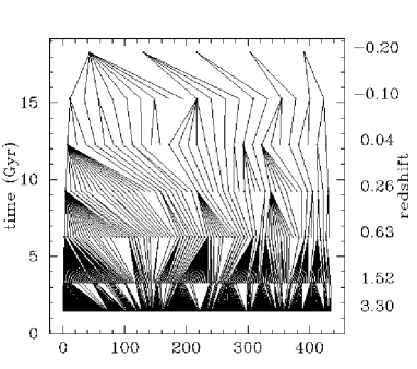
Figure 8: Merging History: $n=-2,\,r_{\mbox{\rm\small thresh}}=5$, haloes $1-5.$ This and the following plots show haloes detected at different points in space-time connected according to the criterion described in §2.1.3, i.e., showing which haloes merge into which. The horizontal axis separates individual haloes, while the vertical axis indicates time/redshift. (Negative redshifts indicate future times.) Circles indicate haloes, with radii a logarithmic transformation of the haloes masses (for display purposes, the specific transformation differs between separate plots) and line segments indicating the merging connections. The haloes at the latest time stage, and the set of predecessors of any halo, are ordered by mass decreasing to the right. Numbering on the horizontal axis indicates the maximum number of haloes in the figure for any time stage.

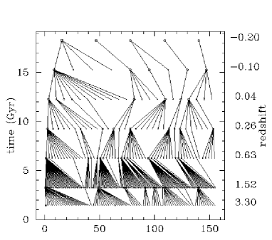
Figure 9: Merging History: $n=-2,\,r_{\mbox{\rm\small thresh}}=1000$, haloes $1-5$

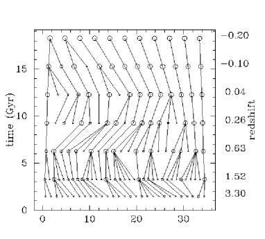
Figure 10: Merging History: $n=-2,\,r_{\mbox{\rm\small thresh}}=5$, haloes $50-60$

Figure 11: Merging History: $n=-2,\,r_{\mbox{\rm\small thresh}}=5$, haloes $400-410$

2.2.3 Merging History Trees

Merging history tree plots (Figs 8–11) are obtained by choosing a range of haloes at the final time stage and tracing back all the progenitors of these haloes. The line segments joining the circles are the key feature of the plots. These indicate that the halo at the earlier time is considered to merge into (or be “identical” to) the halo at the later time according to the 50% criterion explained in §2.1.3. The aim of the plots is to show connectivity over time. So, the horizontal axis is designed to separate the haloes according to their future merging activity. It doesn’t directly indicate space positions, although there should be some correlation between how close two haloes are in the plot and how close they are in space (since haloes need to be close in order to merge together later on).

Much information on the merging process is represented in these tree plots. However, they do not show the entire complexity of the merging process (or “graph” in mathematical terminology). Since the halo merger history trees presented here start with a range of final haloes and trace backwards, haloes which have no descendant at the final time stage are not shown. As summarised in Table 4, a significant fraction of the haloes at a given time stage have no descendants at the following time stage. A simple explanation is that a large fraction of a halo can evaporate in the merging process and contribute less than 50% of the mass of the final halo, in which case the merging/identity criterion adopted fails to find a descendant. Typically, about $25\%\pm 25\%$ of a halo evaporates (e.g., in tails) or forms low-density “atmospheres” in N-body simulations of $N\sim 2$ interacting galaxies (Quinn, 1992). These tails or atmospheres are likely to fall below the density detection threshold.

Figs 8 and 9 show that merging ratios of up to around 10:1 occur for many of the most massive haloes at low redshifts, while as indicated by the maximum number of original haloes for any final halo, the merging ratios between early time stages can be much higher, as high as a few hundred to one in several cases for $r_{\mbox{\rm\small thresh}}=5.$

The difference in detection thresholds appears clearly in the difference between the early time stages of Figs 8 and 9. At the nominal redshift $z=11$, many low mass haloes have reached the turnaround density and are thus detected above $r_{\mbox{\rm\small thresh}}=5,$ after which they merge rapidly. In contrast, haloes detected above $r_{\mbox{\rm\small thresh}}=1000$ are mostly detected at $z=1{\cdot}5$; the few which form earlier do not merge in ratios as high as for the $r_{\mbox{\rm\small thresh}}=5$ haloes. Depending on the assumptions one wishes to make regarding the relationship between galaxies and haloes, either of these limiting cases could be interesting.

For merging history trees of the haloes having lower masses at the final time stage (Figs 10 and 11), very little merging occurs apart from the earliest few time stages. Indeed, Fig. 11 shows that many of the smallest haloes either have only recently collapsed or are unmerged objects which have formed well after the first time stage. This can be generalised by stating that the larger a galaxy halo is, the more original haloes it is likely to have been created from, and at any time in general, the more massive a galaxy halo is, the more haloes are likely to be merging into it. (This effect can also be seen in Figs 6 and 7.)

That the lowest mass peaks may form fairly recently or may form early yet undergo no merging at all is to be expected in a “hierarchical galaxy formation” scenario. Bottom-up gravitational collapse does not only imply that small haloes form first and successively merge to form more and more massive haloes, but also that some low mass haloes (e.g., from low amplitude short length-scale perturbations, which must exist if the initial perturbation amplitudes are part of a zero-mean Gaussian distribution) continue to form at late epochs.

The recently forming small haloes in our halo merger trees could be used to model the (observed) existence of low mass, young, low redshift galaxies, such as the dwarf Spheroidals. An interesting case is the SBS 0335-052(W) pair of dwarf galaxies at a redshift of $z=0{\cdot}014$, which have a (stellar) age of not more than $10^{8}$ yr and have a metallicity (O/H) around 1/40 of the solar value ([Izotov et al.] 1997). These two dwarfs are extremely hard to understand as anything other than young, low redshift, low mass galaxies. For such galaxies to provide a constraint on galaxy formation models, precise estimations of number densities and age distributions would be useful—though obviously difficult to obtain without strong observational selection effects.

Figure 12: Spatial two-point autocorrelation functions of haloes in $n=-2,\,r_{\mbox{\rm\small thresh}}=5$ model, shown as $\log_{10}[\xi(r)]$ against $\log_{10}(r),$ where $r$ is the comoving halo pair separation in Mpc. A solid line of slope $-\gamma=-1{\cdot}8$ is shown for comparison.

Figure 13: Evolution of the spatial two-point autocorrelation function, $\xi_{0}\equiv\xi(5$ h^-1Mpc$,z)$ vs redshift ($1+z$). (The highest redshift correlation function for $n=0,\,r_{\mbox{\rm\small thresh}}=1000$ is too noisy to deduce a $\xi_{0}$ value.) Also shown are lines fitted to all but the highest $z$ point for $n=0$ and to the four points with lowest $z$ for $n=-2$.

2.2.4 Halo Correlation Functions

Another important statistic of the haloes is their spatial two-point auto-correlation function, $\xi(r).$ The natural inclusion of $\xi$ in N-body simulations is something not usually present in semi-analytical galaxy formation modelling. Indeed, [Yano et al.]’s (1996) application of [Jedamzik]’s (1995) approach to the “cloud-in-cloud” problem of the Press-Schechter formalism ([Press & Schechter] 1974) shows that the mass function of the latter suffers significantly from the lack of inclusion of $\xi.$ [Nagashima & Gouda] (1997) confirm this in semi-analytical merging history tree simulations using [Rodrigues & Thomas]’s (1996) modification of the Block model ([Cole & Kaiser] 1988).

Fig. 12 shows the correlation functions for the haloes detected for $n=-2,\,r_{\mbox{\rm\small thresh}}=5.$ These functions have slopes $-\gamma\approx-1{\cdot}8,$ where

$$\xi=(r_{0}/r)^{\gamma}(1+z)^{-(3+\epsilon-\gamma)},$$ (1)

$r$ and $r_{0}$ are expressed in comoving coordinates, and $\epsilon$ parametrises the growth rate of $\xi_{0}(z)\equiv\xi(r_{0},z)$, deduced either from observation or theory ([Groth & Peebles] 1977).

The slopes of $\xi$ for the other combinations of $n$ and $r_{\mbox{\rm\small thresh}}$ are similar, so are consistent with that observed for galaxies, i.e., $1{\cdot}7\,\lower 2.58334pt\hbox{$\buildrel<\over{\sim}$}\,\gamma\,\lower 2.58334pt\hbox{$\buildrel<\over{\sim}$}\,1{\cdot}8$ (e.g., [Peebles] 1980; [Davis & Peebles] 1983; [Loveday et al.] 1992). Some observations indicate that $\gamma$ evolves with time ([Infante & Pritchet] 1995), but others do not detect this ([Hudon & Lilly] 1996). N-body simulation derived correlation function slopes vary around the same values, but are sensitive to whether the correlation is that of particles (identified as galaxies), of haloes or of mass-density ([Davis et al.] 1985; [Efstathiou et al.] 1988; [Suto & Suginohara] 1991; [Suginohara & Suto] 1991; [Melott] 1992).

The haloes of our N-body derived merging history trees therefore have realistic correlation slopes and do not suffer from the lack of a correlation function of the traditional semi-analytical methods.

Another interesting property of the correlation function is the growth rate of $\xi_{0},$ parametrised by $\epsilon.$ This is shown in Fig. 13. Since the simulations used here are not normalised conventionally, the values of $\xi_{0}(z=0)$ are less useful than the change of $\xi_{0}$ with redshift.

To the extent that Eq. 1 is a good approximation, direct observational estimates of $\epsilon$ at varying $z_{\mbox{\rm\small med}}$ (median redshift) include $\epsilon=1{\cdot}6\pm 0{\cdot}5$ ([Warren et al.] 1993, $z_{\mbox{\rm\small med}}$$=0{\cdot}4$), $\epsilon=-2{\cdot}0\pm 2{\cdot}7$ ([Cole et al.] 1994, $z_{\mbox{\rm\small med}}$$=0{\cdot}16$), $\epsilon\approx 2{\cdot}2$ ([Shepherd et al.] 1997, $z_{\mbox{\rm\small med}}$$=0{\cdot}37$) and $\epsilon=2{\cdot}8$ [cf. §4.1(3), [Le Fèvre et al.] (1996), adopting $r_{0}=5{\cdot}0h^{-1}$ Mpc and $c$$z_{\mbox{\rm\small med}}$(Stromlo-APM)$=15,200$ km s^-1([Loveday et al.] 1992, 1995), $z_{\mbox{\rm\small med}}$(CFRS)$=0{\cdot}56$]. By hypothesising major changes in visible galaxy populations from low to high redshifts, these values of $\epsilon$ could be lowered.

Simple theoretical values of $\epsilon$ include those expected for clustering fixed in comoving coordinates ($\epsilon=\gamma-3\approx-1{\cdot}2$, so that the index in Eq. 1 is zero); clustering fixed in proper coordinates on small scales [“stable clustering”, $\epsilon=0$; since the numbers of “clusters” changes by $(1+z)^{3}$ and the number of galaxy pairs by $(1+z)^{6}$, the factor in Eq. 1 for $r$ in proper coordinates is $(1+z)^{-3}$]; and linear growth of initial fluctuations for an $\Omega_{0}=1$ universe ($\epsilon=\gamma-1\approx 0{\cdot}8$).

Table 7: Low redshift spatial correlation function growth rates $\epsilon$ (see Eq. 1). Only the four lowest redshift points are used for $n=-2.$

$$\begin{array}[]{ c cc }\hline\cr r_{\mbox{\rm\small thresh}}\mbox{\rule[-6.45831pt]{0.0pt}{4.30554pt}}&n=0&n=-2\\ \hline\cr 5&-0{\cdot}6\pm 0{\cdot}1&-0{\cdot}6\pm 0{\cdot}6\\ 1000&-0{\cdot}4\pm 0{\cdot}3&-0{\cdot}3\pm 0{\cdot}3\\ \hline\cr\end{array}$$

More detailed analyses include those of [Peacock] (1996) and [Matarrese et al.] (1997), who discuss departures from the power law of Eq. 1, bias factors and differences between the linear, quasi-linear and non-linear overdensity regimes. In particular, the transition between the linear and non-linear regimes can give rise to $\epsilon\approx 2{\cdot}8$ [for $\gamma=1{\cdot}8$ in Eq. (29) of [Peacock & Dodds] (1996) and $\Omega_{0}=1$].

By contrast to the above estimates, the values of $\epsilon$ for our haloes are those for which haloes merge between time steps. This means that as haloes approach each other and merge, halo pairs are replaced by single haloes, so that the correlation decreases more slowly than if the haloes’ identities were kept separate. Because of this, the values of $\epsilon$ derived here (Table 7) lie between those expected for clustering fixed in comoving and proper coordinates respectively, and are lower than the more precise of the observational estimates.

Implications of the effect of merging, in particular on the angular correlation function, have been presented in more detail in [Roukema & Yoshii] (1993).

Another property to note is that for the $n=-2$ model, $\xi_{0}$ initially decreases until $z\sim 1,$ after which it increases to the present. This is because during the transition from linear perturbation amplitudes to non-linear collapse, small length-scale perturbations on top of large length-scale perturbations have their density boosted, and so can collapse well before small length-scale perturbations in low density regions. During this period, perturbations in the low-density regions are not represented by collapsed objects. Hence, the mean number density of collapsed objects used to normalise the correlation function represents the numbers of haloes in only the high-density regions, but includes the volume in both low and high-density regions. The mean density is therefore biased low, so the correlation function amplitude is biased high. As a larger fraction of perturbations collapse, this initially high bias in $\xi$ decreases until normal correlation growth takes place.

This effect is not seen for $n=0$ because large length-scale perturbations have relatively less power for $n=0$ than for $n=-2.$ Possible consequences of such a “Decreasing Correlation Period” (also reported by [Roukema] 1993 and [Brainerd & Villumsen] 1994) on observations of the angular correlation function are discussed in [Ogawa et al.] (1997). From Fig. 13, the rate of correlation decrease is $d(\log_{10}\xi_{0})/d[\log_{10}(1+z)]\sim 0{\cdot}3\pm 0{\cdot}15$ to $z\sim 0{\cdot}5-1.$

Figure 14: Method by which time steps could be interpolated. Histogram of time of radial infall of haloes (at $t=9{\cdot}3$ Gyr for $n=-2,$ $r_{\mbox{\rm\small thresh}}=1000$) considered as point particles which fall into isothermal potentials of the combined masses (at $t=12{\cdot}3$ Gyr) of the multiple merger products.

2.2.5 Merging Between Output Time Steps

The merging history trees of haloes could in principle be analysed with a higher time resolution than in the figures presented here, merely by using many more output time steps from the N-body simulation. The only drawback would be practical handling of computer disk space. A single time step for the [Warren et al.] (1992) simulations normally occupies 32 Megabytes.

Here we note an alternative to using more output times. Interpolation between time steps, making analytical assumptions for the trajectories of the haloes, can give interpolated merger times which are statistically consistent with the more accurate trajectories calculated in the full N-body simulation. Fig. 14 shows that the approximation of point particles falling into isothermal potentials gives an approximately decreasing merger rate, which is consistent with the overall merging rate. A small fraction of objects have estimated merger times greater than the output time step interval, i.e., greater than the time required for a merger according to the full N-body simulation. This is a limitation to (at least this) analytical interpolation, but the fraction of such cases is small enough that this interpolation technique may be a fair approximation statistically.

However, N-body analyses of few-galaxy systems (e.g., [Prugniel & Combes] 1992; [Hernquist & Weinberg] 1989) suggest that merger times may be difficult to predict by any simple analytical method, so caution is needed. Although the results should not differ significantly from those of the authors just cited, use of such interpolations for the calculation of N-body merger history trees could be verified by comparison with the intermediate time steps of the N-body systems. Interpolation is not adopted for this paper.

3 Galaxy Formation Application (Star Formation and Evolution)

The example of a galaxy formation recipe adopted here combines (a) gravity: halo merging history trees are derived from density peaks detected above a given overdensity threshold in $1{\cdot}1$ million particle pure gravity N-body simulations; and (b) other physical processes: one galaxy is assumed to form in each halo; we insert an observationally inspired star formation rate due to merger-induced starbursts (and/or a quiescent star formation rate); and we combine this with the initial mass function and stellar evolution modelled in Bruzual’s (1983) evolutionary population synthesis code.

3.1 Modelling Starbursts to Occur on Merging

Star formation physics is represented by an initial mass function (IMF) and a star formation rate (SFR). The separability of these two functions appears to be a reasonable assumption according to both observation and theory, e.g., the recent ISO (Infrared Satellite Observatory) observations of both infrared-ultra-luminous and “normal” star-forming galaxies are consistent with existence of a universal IMF ([Lutz et al.] 1996; [Vigroux et al.] 1996; [Gilmore] 1996). The IMF is discussed in §3.2, while this section describes the modelling of the SFR, based on starbursts.

For the purpose of this first-order examination of the effect of merger-induced starbursts on galaxy luminosity evolution, we only use very simple models of the starbursts. Observational and theoretical motivations are as follows.

An early observational model of a starburst (not necessarily caused by a merger), is that of Rieke et al. (1980).

Rieke et al. (1980) model the starburst in the nucleus of M82 via evolutionary population synthesis. They find that instantaneous (Dirac delta function) and constant star formation rate models fail to produce the observed spectrum, but exponential decay SFR models with an IMF with a low-mass cutoff well above a solar mass are necessary. Their best models (say, D and F) have the e-folding time in the SFR $t_{0}=2{\scriptstyle\times}10^{7}$yr and $t_{0}=1{\scriptstyle\times}10^{8}$yr and run for $t=5{\scriptstyle\times}10^{7}$yr and $t=1{\cdot}6{\scriptstyle\times}10^{7}$yr respectively. Both have IMF’s with $\alpha=2$ and the mass range $3{\cdot}5-31M_{\odot}.$ The mass turned into stars is $\approx 1{\cdot}5-2{\scriptstyle\times}10^{8}M_{\odot},$ this being constrained to be less than the total mass in the nucleus, estimated as $3{\scriptstyle\times}10^{8}M_{\odot}$ by Rieke et al. This constraint is the major reason for the need of a high low-mass cutoff. If a normal low-mass cutoff is used, then the mass actually present in the nucleus is insufficient to generate the observed luminosity.

Rieke (1991) describes more recent observational constraints on the models for M82, finding that the above conclusion still holds using more modern stellar evolutionary tracks in the models.

Scoville & Soifer (1991) argue from IRAS far-infrared data that “virtually all of the strong global starbursts occur in … starburst-infrared galaxies,” where the latter are defined as “those with $L_{IR}/M_{H_{2}}$ significantly higher than in normal galaxies,” and that starburst-infrared galaxies correlate highly with “the occurrence of a recent [galaxy-galaxy] interaction.” They argue that such global starbursts require the progenitor galaxies to be of comparable mass in order to generate such activity.

While this result doesn’t necessarily imply the converse, i.e., that all mergers of similarly sized galaxies induce major global starbursts, the converse is a fair hypothesis. With the assumption of this converse, Scoville & Soifer find that the high luminosity end of the infrared (galaxy) luminosity function from the IRAS survey is consistent with $0{\cdot}2\%$ of all spiral galaxies undergoing global starbursts at the present with lifetimes equal to the dynamical times of large galaxies, $\sim 1-2{\scriptstyle\times}10^{8}$yr. For the most IR-luminous galaxies they find SFR’s of $10-100M_{\odot}$yr${}^{-1}.$ They don’t find a high low-mass cutoff necessary for their models to fit the observations.

Norman (1991), citing the models of merging gas-rich disk galaxies of Hernquist and Barnes, ([Barnes] 1990, equal mass galaxies; Hernquist 1989, differing mass galaxies), describes a qualitative three-phase model to take into account gas falling into the galaxy centre. The three phases essentially correspond to proportions of the gas having fallen to the centre. Published star formation models following these three phases separately are not cited in the article, but would obviously be of interest.

Norman (1991) also argues that constant SFR models of starbursts satisfy an observed sparsity of post-starburst galaxies relative to starburst galaxies, but that instantaneous SFR models predict too many post-starbursts.

Hence, for this example application of an N-body derived halo merger history tree, a starburst with a constant SFR is chosen.

For pairwise mergers, the following canonical values are chosen. We normalise the rate of the starburst for a “typical” large galaxy merger product to be an SFR of $\psi_{0}=50M_{\odot}$yr^-1 as in the models of Scoville & Soifer (1991). The low-mass cutoff in the IMF used here ($0{\cdot}08M_{\odot}$, see Eqn 9) is consistent with Scoville & Soifer’s value of $0{\cdot}1M_{\odot}.$

We consider the merger product to be the remnant of two large galaxies each of gas mass $M^{\mbox{\rm\small gas}}_{0}=10^{10}M_{\odot},$ total mass $M^{\mbox{\rm\small halo}}_{0}=10^{12}M_{\odot}$ and halo radius $50\,$kpc. This gives a dynamical time $t_{\mbox{\rm\small dyn}}\equiv(G\rho_{0})^{-1/2}\approx 2{\scriptstyle\times}10^{8}$yr, where the mean density of either galaxy to its halo radius is $\rho_{0}=8{\scriptstyle\times}10^{6}M_{\odot}$kpc${}^{-3}.$ The modelling by [Barnes] (1990), Hernquist (1989) or earlier non-gaseous N-body models such as those of Quinn & Goodman (1986) find that the merger takes place over only a few dynamical times. So the choice of progenitor galaxies here gives a $t_{\mbox{\rm\small dyn}}$ matching Scoville & Soifer’s burst duration of $t^{\mbox{\rm\small burst}}_{0}=2{\scriptstyle\times}10^{8}$yr, which is chosen as the canonical burst duration.

In this canonical case, $50\%$ of the total gas mass is used up in the burst. To sum up, we have

$$\psi_{0} = 50M_{\odot}\mbox{\rm yr}^{-1}$$ (2)

$$M^{\mbox{\rm\small gas}}_{0} = 10^{10}M_{\odot}$$ (3)

$$M^{\mbox{\rm\small halo}}_{0} = 10^{12}M_{\odot}$$ (4)

$$\rho_{0} = 8{\scriptstyle\times}10^{6}M_{\odot}\mbox{\rm kpc}^{-3}$$ (5)

$$t^{\mbox{\rm\small burst}}_{0} = 2{\scriptstyle\times}10^{8}\mbox{\rm yr.}$$ (6)

The canonical values are then scaled for haloes of arbitrary mass. To first order it seems reasonable that the kinetic energy available for generating star formation should be proportional to the mass of the smaller halo and that the SFR should also be proportional to the total amount of gas available. So, the SFR is scaled by the mass of the smaller halo times the ratio of combined gas mass to $2M^{\mbox{\rm\small gas}}_{0}$.

Since we consider the duration of the starburst to be the order of a dynamical time, $t^{\mbox{\rm\small burst}}$ is scaled by $\rho^{-1/2},$ where $\rho$ is the density of the larger halo.

Given a coarse time resolution in the merging histories, each merger is identified by the code as a multiple merger—e.g., seven haloes merge to one—instead of as a series of several individual pairwise mergers. If we consider the approximation that each of the pairwise mergers involves the largest progenitor halo, then a compromise can be carried out as follows.

(a) Have a single burst with the above normalisation. Scale the SFR by the sum of the masses of each of the smaller haloes (i.e., all but the largest) and by the ratio of the combined gas mass from all progenitor haloes (i.e., including the largest) to $2M^{\mbox{\rm\small gas}}_{0},$ giving

$$\psi(t)=\psi_{0}{\sum_{i\neq i^{\mbox{\rm\tiny max}}}M^{\mbox{\rm\small gal}}_{i}\over M^{\mbox{\rm\small halo}}_{0}}{\sum_{{\rm all}\,i}M^{\mbox{\rm\small gas}}_{i}\over 2M^{\mbox{\rm\small gas}}_{0}}$$ (7)

where $\psi(t)$ is the star formation rate (in $M_{\odot}$yr^-1), the progenitor haloes are labelled by $i$, and $i^{\mbox{\rm\small max}}$ is the label of the progenitor halo of greatest mass. (For the group-finding algorithm used in this article, $i^{\mbox{\rm\small max}}=1.$)

(b) Scale the starburst duration as above, by $\rho^{-1/2},$ where $\rho$ is the density of the largest halo, giving

$$t^{\mbox{\rm\small burst}}=t^{\mbox{\rm\small burst}}_{0}\left({\rho_{\mbox{\rm\small halo}}\over\rho_{0}}\right)^{-1/2}.$$ (8)

Two modifications may have to be applied in some situations. Firstly, where the starburst at this rate uses up more gas than is actually available, it is truncated at the point of time when zero gas mass is left. Secondly, if the duration of the starburst is longer than the time interval to the next time step, it is truncated at that next time step.

While this modelling of multiple merger-induced starbursts with large time steps may make the luminosity evolution more temporally discrete than it should be, it does conserve physical quantities in line with the observational and theoretical constraints discussed above, and should be sufficient for this demonstration of the use of N-body based merger history trees.

3.2 Connection with Stellar Evolutionary Population Synthesis

We use stellar evolutionary population synthesis to combine star formation and stellar evolutionary physics. A version of Bruzual’s stellar evolutionary population synthesis code (Bruzual 1983) which is essentially that of 1983, but with some updating and conversion to Unix, is the primary population synthesis code used, but the code of [Guiderdoni & Rocca-Volmerange] (1987) and [Rocca-Volmerange & Guiderdoni] (1988) (1993 version) gives similar results. In the interactions of the programs presented above with this code, the SFR history and masses of galaxies and gas are determined outside of the Bruzual routines or by amended versions of the Bruzual routines. The return of gas from supernovae to a galaxy was turned off for test purposes but otherwise left on. The loss of this supernova gas from a galaxy was not invoked, neither was the option allowing infall of gas to a galaxy.

The initial mass function (IMF) used was the default IMF chosen by the code, after Scalo (1986) (e.g., Fig. 16 in Scalo, 1986). Where $f(m)\propto m^{-(1+x)}$ is the number of stars born per unit (linear) mass in a given mass range, the IMF slopes used are

$$x=\left\{\begin{array}[]{lll}-2{\cdot}60,&0{\cdot}05\leq M\leq 0{\cdot}08M_{\odot}&\mbox{(brown dwarfs)}\\ -2{\cdot}60,&0{\cdot}08\leq M\leq 0{\cdot}18M_{\odot}\\ 0{\cdot}01,&0{\cdot}18\leq M\leq 0{\cdot}42M_{\odot}\\ 1{\cdot}75,&0{\cdot}42\leq M\leq 0{\cdot}62M_{\odot}\\ 1{\cdot}08,&0{\cdot}62\leq M\leq 1{\cdot}18M_{\odot}\\ 2{\cdot}50,&1{\cdot}18\leq M\leq 3{\cdot}5M_{\odot}\\ 1{\cdot}63,&3{\cdot}50\leq M\leq 75M_{\odot}.\end{array}\right.$$ (9)

The Bruzual code normally works by using simple analytical expressions for the SFR history, so that no numerical effects (e.g., rounding errors) can be introduced at this stage. Numerical effects can of course be present when the galaxy spectral energy distribution is calculated, since only finitely many points representing different stellar ages are present for each of the finitely many mass tracks.

However, this has the disadvantage that one cannot simply stop the code after a certain time step, save the population data, start up the program from scratch, read in the saved population data and continue on as if the program had never stopped. The population data could be stored and later read back in, but this would round each star’s age to the appropriate stellar evolution track age at every time step, making cumulative errors.

Bruzual’s code was therefore modified slightly in order to allow use of numerical SFR histories. For each time step and each halo, an array of time points from that time step to the following time step and the corresponding array of integrals of the SFR are stored. These integrals of the SFR are the total number of stars created since the first star formation in any of the progenitor peaks which end up in the present peak being worked on. Because the integral of the SFR is used, the errors are not cumulative, and in the present version are $\sim 0{\cdot}1\%.$

The program which applies stellar evolutionary population synthesis to the merging histories stores an SFR history for each peak as it is evolved to the next time step, adds these together for merged peaks, and from that point on evolutionary population synthesis applies just as it would for an isolated galaxy, except that the merging history tree information is contained implicitly in the complex shape of the SFR history.

For the present model, population synthesis is applied by optionally having an exponentially decreasing SFR between mergers and optionally having starburst SFR’s commencing at each merger. Gas masses and total masses are by default conserved, i.e., the gas and total masses of a galaxy are the respective sums of the gas and total masses of predecessor galaxies, except that matter accreting directly onto the density peaks is added as gaseous mass. If both exponential and burst star formation are turned on simultaneously (probably the most realistic model) the SFR’s are simply added together, conserving the number of stars created.

3.3 Luminosity Functions

This combination of N-body generated merging history trees with other elements of a simple galaxy formation recipe is sufficient to generate luminosity functions which are comparable to the estimated present-day luminosity function, and so could be extended to an exploration of galaxy formation parameter space, in which the parameters are free rather than motivated by observation as in the present work.

The merging history trees presented above are derived from power law initial spectrum N-body simulations intended for comparison of the relative properties of haloes of different masses, so need to be renormalised in a cosmological context. For simplicity, an increase in the length scale by a factor of two is the renormalisation adopted. Masses scale as the cube of the length in order to leave the numerical operations in the N-body simulations and the merger history tree analysis unchanged and time is not rescaled. This brings the number density of the haloes close to that of observed galaxies.

Figure 15: Star formation rate (SFR) history for the most massive galaxy at the final time step in the $n=-2,\,r_{\mbox{\rm\small thresh}}=5,$ exponential+burst model, $\mu=0{\cdot}15.$ The SFR in stars yr^-1 is plotted against time since the formation of the first progenitor of the galaxy.

Figure 16: ${\cal M}_{\mbox{\rm\small lum}}/L_{\mbox{\rm\small IIIaJ}}$ for rest frame values of $L_{\mbox{\rm\small IIIaJ}}$ for a run on the $n=-2,\,r_{\mbox{\rm\small thresh}}=5$ model merging history with exponential and burst evolution turned on and Bruzual’s SFR parameter $\mu=0{\cdot}15.$ The masses detected at the time stage $t_{i}$ and the luminosities resulting at the end of the interval $[t_{i},t_{i+1})$ are used to obtain ${\cal M}_{\mbox{\rm\small lum}}/L_{\mbox{\rm\small IIIaJ}}$ values labelled $t_{i}$ in this figure.

A baryon fraction of 10% is adopted. Nucleosynthesis results (e.g., [Walker et al.] 1991) and $H_{0}$ estimates ([Tanvir et al.] 1995; [Kundić et al.] 1997) make this a reasonable round number for a critical density universe with a null cosmological constant. [Some other estimates of similar baryon fractions include Galaxy estimates of $0{\cdot}7$ out to a Holmberg radius, or down to possibly $0{\cdot}07$ for the whole Galaxy ([Freeman] 1987); $0{\cdot}25$ for galaxy clusters (e.g., [Sarazin] 1987); and $\sim 0{\cdot}1$ over the whole range of cosmological structures from dwarf spheroidals to rich clusters ([Blumenthal] 1988).]

Figure 17: IIIaJ luminosity functions for the $n=-2,\,r_{\mbox{\rm\small thresh}}=5$ model, exponentially decaying plus burst SFR, Bruzual’s SFR index $\mu=0{\cdot}15.$ The model curves are of the line styles indicated, labelled by the beginning of each time stage interval, and compared with a Schechter function with locally estimated parameters (solid line, Eq. 10). Luminosities are expressed in absolute magnitudes, ${\cal M}_{\mbox{\rm\small IIIaJ}},$ in the observer’s frame, i.e., K-corrected ([Wirtz] 1918); densities are in $\log_{10}$(N Mpc^-3 mag^-1) in comoving coordinates.     The following plots show the same quantities for different $n$ and $r_{\mbox{\rm\small thresh}}$.

Figure 18: IIIaJ luminosity functions for $n=-2,\,r_{\mbox{\rm\small thresh}}=5$ model, (exponential decay only SFR), Bruzual’s $\mu=0{\cdot}15.$

Figure 19: IIIaJ luminosity functions for $n=-2,\,r_{\mbox{\rm\small thresh}}=5$ model, burst-only SFR. In this and the following plots of the luminosity function for burst-only models, the luminosity functions at the first time stage are missing. This is a property of the model: stars are only formed when mergers occur; this first occurs at the second time stage.

All baryonic matter is assumed to be potentially star-forming material.

An example of an SFR history (for the galaxy resident in the most massive final halo in the $n=-2,\,r_{\mbox{\rm\small thresh}}=5$ exponential-plus-burst model) is shown in Fig. 15. Both the exponentially declining “quiescent” star formation rates and the merger-induced bursts are clearly visible. Bruzual’s SFR parameter has the value $\mu=0{\cdot}15$ [$\mu$ is the proportion of gas turned into stars in a (non-merging) galaxy within $1\,$Gyr].

Mass-to-light ratios, ${\cal M}_{\mbox{\rm\small lum}}/L_{\mbox{\rm\small IIIaJ}},$ (using rest frame values of $L_{\mbox{\rm\small IIIaJ}}$, i.e., no K-corrections) for the galaxies in this model at different time steps are shown in Fig. 16. These mass-to-light ratios are somewhat high relative to optical galaxy estimates (e.g., $2\,\lower 2.58334pt\hbox{$\buildrel<\over{\sim}$}\,{\cal M}_{\mbox{\rm\small disk}}/{L_{B_{\mbox{\rm\small disk}}}}\,\lower 2.58334pt\hbox{$\buildrel<\over{\sim}$}\,7\,M_{\odot}L_{\odot}^{-1}$ derived from the inner part of the optical/HI rotation curves of disk galaxies without bulges, [Freeman] 1987; stellar population values, [Larson & Tinsley] 1978) but similar to those estimated from X-ray emission in ellipticals ($20\,\lower 2.58334pt\hbox{$\buildrel<\over{\sim}$}\,{\cal M}_{\mbox{\rm\small tot}}/L_{B}\,\lower 2.58334pt\hbox{$\buildrel<\over{\sim}$}\,30\,M_{\odot}L_{\odot}^{-1}$ within a radius $r\sim 30-40$ kpc, [Canizares] 1987).

The corresponding luminosity functions for the galaxies in this model are shown in Fig. 17, while luminosity functions for either exponentially decaying or burst SFR’s only (not both) are shown in Figs 18 and 19 (for $n=-2,\,r_{\mbox{\rm\small thresh}}=5$). A local luminosity function parametrised as a Schechter function

$$dN/dL=\phi^{*}(L/L^{*})^{\alpha}\exp(-L/L^{*})d(L/L^{*})$$ (10)

([Schechter] 1976) where $\phi^{*}=1{\cdot}56{\scriptstyle\times}10^{-2}h^{3}$ Mpc^-3, $M^{*}=-19{\cdot}6+5\log_{10}h$ and $\alpha=-1{\cdot}1$ ([Efstathiou et al.] 1988), is shown for comparison. [This estimate is similar to the more recent Stromlo-APM estimate of [Loveday et al.] (1992), while the CfA2 estimate of [Marzke et al.] (1994) differs from both in having a value of $M^{*}$ about $0{\cdot}7$ mag fainter.]

The luminosity functions for the $n=-2,\,r_{\mbox{\rm\small thresh}}=5$ exponential-plus-burst and exponential-only SFR’s are similar to one another (Figs 17, 18), as the rate of the exponential SFR alone is enough to use up most of the gas, leaving little possibility for the bursts to make any difference between galaxies of differing merging histories. The luminosity function slopes are steeper than the observational faint end slopes (for field galaxies), and are similar to the steep slopes expected from the mass functions (Figs 2 - 4). The other three combinations of $n$ and $r_{\mbox{\rm\small thresh}}$ for the exponential-plus-burst and exponential-only models give similarly steep luminosity functions. This result is similar to that of other semi-analytical models (e.g., [Kauffmann et al.] 1993).

The “bump” at the bright end of some of the later luminosity functions (particularly in Fig. 18) combined with the steep slope is suggestive of luminosity functions in clusters, but a cluster environment is one in which merger-induced star bursts could be expected to be the more important rather than the less important star formation mode, so it is not clear whether or not this is a useful characteristic of the models.

The faint end sudden drop (at $M\,\lower 2.58334pt\hbox{$\buildrel<\over{\sim}$}\,-16$ in these two figures) is simply due to the resolution limit of the models.

The $n=0,\,r_{\mbox{\rm\small thresh}}=5$ burst-only model (Fig. 20) is quite striking in having a “faint end” slope almost precisely as shallow as the slope of the observational luminosity function. In addition, the bright ends of the earlier of these luminosity functions have steep drops as in the observational luminosity function, though this occurs for galaxies a few magnitudes too bright.

How significant are the luminosity functions of the $n=0,\,r_{\mbox{\rm\small thresh}}=5$ burst-only model? For a flat rotation curve for the Galaxy with density falling off as $r^{-2},$ the detection threshold of $r_{\mbox{\rm\small thresh}}=5$ corresponds to a Galaxy halo radius of about $1500\,$kpc, larger than any claimed value. Apart from the recent observational suggestion of [Honma & Sofue] (1996) that the halo is only 15 kpc in radius, a conventional estimate of $r_{halo}\sim 100-300$ kpc would still imply that the detection threshold used here overestimates the mass of the Galaxy by an order of magnitude [since $\rho\propto r^{-2}\Rightarrow M(<r)\propto r$]. Also, members of the Local Group would missed, since one galaxy per halo and maximal merging are assumed.

These problems could conceivably be corrected by a reduction in galaxy masses, which would reduce the luminosities, and by an increase in the normalisation to account for the missing Local Group galaxies, whose analogues would presumably be detected (in the model) in isolation in other regions of space. However, while the former would improve the fit, the latter would worsen it.

The $n=0,r_{\mbox{\rm\small thresh}}=1000$ burst-only model does include these smaller galaxies (“halo substructure”) and results in a luminosity function which is slightly too steep (Fig. 22). The $n=-2$ models (Figs 19, 21) also have slopes which are relatively shallow, but none as shallow as that for the $n=0,\,r_{\mbox{\rm\small thresh}}=5$ model.

The reason why the burst-only models have shallower slopes can be explained fairly simply: smaller mass haloes typically undergo less merging, so become relatively underluminous relative to higher mass haloes. Star formation dominated by merger-induced bursts could therefore provide a simple way of reducing the faint-end slopes expected from the Press-Schechter function.

Figure 20: IIIaJ luminosity functions for $n=0,\,r_{\mbox{\rm\small thresh}}=5$ model, burst-only SFR.

Figure 21: IIIaJ luminosity functions for $n=-2,\,r_{\mbox{\rm\small thresh}}=1000$ model, burst-only SFR.

Figure 22: IIIaJ luminosity functions for $n=0,\,r_{\mbox{\rm\small thresh}}=1000$ model, burst-only SFR.

As might be expected from the similarity in the mass functions (Figs 2, 4, 5) for three of the burst-only models, the luminosity functions are also similar to one another. However, a characteristic of the mass function of the $n=-2,\,r_{\mbox{\rm\small thresh}}=5$ model appears (marginally) to be shared by the corresponding luminosity function: the slope seems to become shallower with time. If this were significant, it could be of considerable interest in reconciling faint galaxy counts (e.g., [Tyson & Seitzer] 1988; [Tyson] 1988) with the flatness of the locally estimated luminosity function, though it would also need to show evolution in the bright end of the luminosity function as deduced from recent redshift surveys ([CFRS-VI] 1995, [Ellis et al.] 1996 and [Cowie et al.] 1996).

The evolution in slope could be attributed to the evolution in the Press-Schechter mass function shown in Fig. 2, with the addition of a systematic reduction in slope induced by our burst-only SFR formalism.

Both the flatness of the $n=0,\,r_{\mbox{\rm\small thresh}}=5$ burst-only luminosity functions and the decreasing slope of the $n=-2,\,r_{\mbox{\rm\small thresh}}=5$ model suggest that these parameter combinations should be interesting for future explorations of galaxy formation models using N-body derived merger history trees.

4 Conclusion

The algorithms and results discussed above show that this method of deriving halo merging history trees directly from N-body simulations is feasible and easily combined with evolutionary stellar population synthesis for exploration of a simple galaxy formation model. The method has been applied to [Warren et al.]’s (1992) N-body simulations with $n=0$ and $n=-2$ power law initial perturbation power spectra, using $r_{\mbox{\rm\small thresh}}=5$ and $r_{\mbox{\rm\small thresh}}=1000$ overdensity detection thresholds to detect dark matter haloes.

Several subsets of the merging history trees have been plotted, directly showing quantitative patterns of halo merging from fully non-linear calculations. The merging history trees were combined with simple, observationally normalised proportionality assumptions for star formation rates and stellar evolutionary population synthesis in order to demonstrate a simple galaxy formation “recipe”, in which star formation is either exponentially decreasing, induced by mergers, or both. In addition, interesting properties of halo formation and evolution were noted.

The galaxy formation recipe adopted shows that if most star formation occurs as merger-induced bursts, then some flattening of the faint end of the galaxy luminosity function relative to that expected from the mass functions may be obtained. Indeed, for the analysis using (a) a white noise perturbation spectrum slope ($n=0$) and (b) a detection threshold typical of that for a perturbation just reaching the turn-around density ($r_{\mbox{\rm\small thresh}}=5$), the resulting present-day luminosity function has a faint-end slope similar to $\alpha=-1{\cdot}1,$ i.e., that estimated for local, field, high surface brightness galaxies. Moreover, for the same value of $r_{\mbox{\rm\small thresh}}$ and a perturbation slope similar to that of CDM, there marginally appears to be a steepening of the faint end slope for increasing redshift.

However, since this is only a simple test application of merging history trees to galaxy formation modelling, and the N-body simulations are designed for the study of relative rather than absolute halo properties, these results should be taken as indicative of worthwhile galaxy formation “recipes” to explore further, rather than as a definite explanation for a luminosity function with a flat faint end.

Other interesting by-products from this method of analysing non-linear gravitational collapse are properties of hierarchical halo formation.

(1) Individual merger rates can be very different from average merger rates and the fraction of mass coming from accretion can be quite high. For example, for $n=0,\,r_{\mbox{\rm\small thresh}}=5$, the mean number of haloes which collapse at any time stage and end up in a halo at the final time stage is $7{\cdot}4,$ the standard deviation in this quantity is $20{\cdot}7$ (Table 5) and the maximum is 233. For the same halo detection parameters, a mean fraction of 32% of the mass in the final haloes comes directly from accretion of uncollapsed matter (Table 6), but this fraction varies widely between different haloes. (For the other three parameter choices, the merger ratios are about a factor of two lower, while the accretion percentages are about the same.)

(2) Low mass haloes may either form at very recent cosmological epochs or may undergo no mergers at all throughout a Hubble time. The former may be counter-intuitive, but can be simply understood as being due to the existence of small amplitude, small length-scale perturbations at early epochs, expected for a zero-mean Gaussian amplitude distribution. Some (if not many) perturbations have small initial amplitudes: these only become non-linear recently. Thus, observations such as that of a young, low redshift, low metallicity dwarf galaxy pair ([Izotov et al.] 1997) can be explained naturally within a hierarchical halo formation model.

(3) If there is sufficiently more power on large than small scales, e.g., $n=-2,$ then the first fluctuations to collapse (forming haloes) are only those inside of large length-scale perturbations, so that the spatial distribution of the haloes is initially much less uniform than that of the linear (and non-linear) fluctuations in general. In other words, the amplitude of the spatial correlation function of the haloes may start from a highly biased value (relative to the linear perturbation theory expectation), and decrease in bias until a transition redshift when “normal” correlation growth commences. Observational consequences of such a “Decreasing Correlation Period” are discussed in [Ogawa et al.] (1997).

Many further developments of the use of N-body derived merger history trees are obvious: different assumptions for processes (2)-(5) cited in the introduction could be adopted; a mechanism (e.g., dissipation) could be chosen to change (6), so that galaxies would not merge every time their parent haloes merged; or at the expense of using more computer disk space, N-body simulations with higher $N$ or larger numbers of output time steps could be used. Use of more physically complex group-finders (e.g., [Gelb & Bertschinger] 1994) should also make some differences to detailed properties of the merger histories. Systematic comparisons between recent analytical predictions (e.g., [Yano et al.] 1996), Merging-Cell-Models models ([Rodrigues & Thomas] 1996) and N-body derived merger history trees could be made. An example of a different assumption for processes (1)-(5) would be to replace the observationally inspired parameters adopted here by free parameters which would be varied to see how sensitive the reduction in the slope of the faint end of the luminosity function is to these parameters.

5 Acknowledgements

We would like to thank Carlos Frenk, George Efstathiou, Cedric Lacey, Tim de Zeeuw, Walter Jaffe, Simon White, Gary Mamon, Peter Thomas, Masahiro Nagashima and Naoteru Gouda for several interesting and useful comments and suggestions. Thank you also to Bob Mann for making many constructive recommendations. This research has been carried out with support from the Australian National University, from the Institut d’Astrophysique de Paris, CNRS, from an ANTARES grant, from a PPARC Research Fellowship, from a Centre of Excellence Foreign Visiting Fellowship at the National Astronomical Observatory of Japan, and has made use of Starlink computing resources.

References

- [Bardeen et al.] Bardeen, J.M., Bond, J.R., Kaiser, N., Szalay, A.S., 1986, Ap.J., 304, 15
- [Barnes] Barnes, J., 1990, Dynamics and Interactions of Galaxies, (Heidelberg, Germany: Springer-Verlag)
- [Barnes & Hut] Barnes, J., Hut, P., 1986, Nat., 324, 446
- [Blumenthal] Blumenthal, G., 1988, The Santa Fe TASI-87, (Singapore: World Scientific Publishing)
- [Bond et al.] Bond, J.R., Cole, S., Efstathiou, G., Kaiser, N., 1991, Ap.J., 379, 440
- [Bond & Myers] Bond, J.R., Myers, S.T., 1996a, Ap.J.Supp., 103, 1
- [Bower] Bower, R.G., 1991, M.N.R.A.S., 248, 332
- [Brainerd & Villumsen] Brainerd, T.G., Villumsen, J.V., 1994, Ap.J., 425, 403
- [Bruzual] Bruzual, G., 1983, Ap.J., 273, 105
- [Canizares] Canizares, C.R., 1987, IAU Symposium 117, 1985, (Dordrecht, Holland: D.Reidel), p165
- [Cen & Ostriker] Cen, R.Y., Ostriker, J.P., 1992, Ap.J., 393, 22
- [Cole et al.] Cole, S.,Aragon-Salamanca, A., Frenk, C.S., Navarro, J.F., Zepf, S.E., 1994, M.N.R.A.S., 271, 781
- [Cole et al.] Cole, S., Ellis, R., Broadhurst, T., Colless, M., 1994, MNRAS, 267, 541
- [Cole & Kaiser] Cole, S., Kaiser, N., 1988, M.N.R.A.S., 233, 637
- [Colless et al.] Colless, M. M., Ellis, R. S., Taylor, K., Hook, R. N., 1990, M.N.R.A.S., 244, 408
- [Colless et al.] Colless, M. M., Ellis, R. S., Broadhurst, T. J., Taylor, K., Peterson, B. A., 1993, M.N.R.A.S., 261, 19
- [Cowie et al.] Cowie, L.L., Songaila, A., Hu, E.M., Cohen,J.G., 1996, A.J., , accepted (astro-ph/9606079)
- [Dalcanton] Dalcanton, J.J., 1993, Ap.J., 415, L87
- [Davis et al.] Davis, M., Efstathiou, G., Frenk, C.S., White, S.D.M., 1985, Ap.J., 292, 371
- [Davis & Peebles] Davis, M., Peebles, P.J.E., 1983, Ap.J., 267, 465
- [Efstathiou et al.] Efstathiou, G., Frenk, C.S., White, S.D.M., Davis, M., 1988, M.N.R.A.S., 235, 715
- [Efstathiou et al.] Efstathiou, G., Ellis, R.S., Peterson, B.A., 1988, M.N.R.A.S., 232, 431
- [Ellis et al.] Ellis, R.S., Colless, M., Broadhurst, T., Heyl, J., Glazebrook, K., 1996, M.N.R.A.S., 280, 235 (astro-ph/9512057)
- [Evrard] Evrard, A.E., 1988, M.N.R.A.S., 235, 911
- [Freeman] Freeman, K.C., 1987, IAU Symposium 117, 1985, (Dordrecht, Holland: D.Reidel), p119
- [1] Frenk, C.S., Baugh, C.M., Cole, S., 1995, astro-ph/9512088
- [Gelb & Bertschinger] Gelb, I.M., Bertschinger, E., 1994, Ap.J., 436, 467
- [Gilmore] Gilmore, G., 1996, Nat., 384, 211
- [Groth & Peebles] Groth, E.J., Peebles, P.J.E., 1977, Ap.J., 217, 385
- [Guiderdoni & Rocca-Volmerange] Guiderdoni, B., Rocca-Volmerange, B., 1987, A.&A., 186, 1
- [2] Hernquist, L., 1989, Nat., 340, 687
- [Hernquist & Weinberg] Hernquist, L., Weinberg, M.D., 1989, M.N.R.A.S., 238, 407
- [Heyl et al.] Heyl, J.S., Cole, S., Frenk, C.S., Navarro, J., 1995, M.N.R.A.S., 274, 755
- [Honma & Sofue] Honma, M., Sofue, Y., 1996, P.A.S.J., 48, L103
- [Hoyle] Hoyle, F., 1953, Ap.J., 118, 513
- [Hudon & Lilly] Hudon, J.D., Lilly, S.J., 1996, Ap.J., 469, 519
- [Infante & Pritchet] Infante, L., Pritchet, C. J., 1995, Ap.J., 439, 565
- [Izotov et al.] Izotov, Y.I., Lipovetsky, V.A., Chaffee, F.H., Foltz, C.B., Guseva, N.G., Kniazev, A.Y., 1997, Ap.J., 476, 698 (astro-ph/9607164)
- [Jedamzik] Jedamzik, K., 1995, Ap.J., 448, 1
- [Kauffmann & White] Kauffmann, G., White, S.D.M., 1993, M.N.R.A.S., 261, 921
- [Kauffmann et al.] Kauffmann, G., White, S.D.M., Guiderdoni, B., 1993, M.N.R.A.S., 264, 201
- [Kundić et al.] Kundić, T. et al., 1997, Ap.J., 482, 75 (astro-ph/9610162)
- [Lacey & Cole] Lacey,C., Cole, S., 1993, M.N.R.A.S., 262, 627
- [Lacey et al.] Lacey, C., Guiderdoni, B., Rocca-Volmerange, B., Silk, J., 1993, Ap.J., 402, 15
- [Lacey & Silk] Lacey, C., Silk, J., 1991, Ap.J., 381, 14
- [Larson & Tinsley] Larson, R.B., Tinsley, B., 1978, Ap.J., 219, 46
- [Le Fèvre et al.] Le Fèvre, O., Hudon, D., Lilly, S.J., Crampton, D., Hammer, F., Tresse, L., , 1996, Ap.J., 461, 534 (CFRS-VIII)
- [CFRS-VI] Lilly, S.J., Tresse, L., Hammer, F., Crampton, D., Le Fèvre, O., 1995, Ap.J., 455, 108 (CFRS-VI)
- [Loveday et al.] Loveday, J., Peterson, B. A., Efstathiou, G., Maddox, S. J., 1992, Ap.J., 390, 338
- [Loveday et al.] Loveday, J., Peterson, B. A., Efstathiou, G. & Maddox, S. J., 1992, Ap.J., 390, 338
- [Lutz et al.] Lutz, D. et al., 1996, A.&A., 315, L137
- [Marzke et al.] Marzke, R.O., Huchra, J.P., Geller,M.J., 1994, Ap.J., 428, 43
- [Matarrese et al.] Matarrese, S., Coles, P., Lucchin, F., Moscardini, L., 286, M.N.R.A.S.1151997 (astro-ph/9608004)
- [Melott] Melott, A.L., 1992, Ap.J., 393, L45
- [Mo & White] Mo, H.J., White, S.D.M., 1996, M.N.R.A.S., 282, 347
- [Nagashima & Gouda] Nagashima, M., Gouda, N., 1997, astro-ph/9608069
- [Navarro & Benz] Navarro, J.F., Benz,W., 1991, Ap.J., 380, 320
- [3] Norman, C.A., 1991, in Massive Stars in Starbursts (Britain: Cambridge Univ. Press)
- [Ogawa et al.] Ogawa, T., Roukema, B.F., Yamashita, K., 1997, Ap.J., 484, 53 (astro-ph/9703158)
- [Peacock] Peacock, J.A., 1996, MNRAS, 284, 885 (astro-ph/9608151)
- [Peacock & Dodds] Peacock, J.A., Dodds, S.J., 1996, MNRAS, 280, L19
- [Peebles] Peebles, P.J.E., 1980, in The Large-Scale Structure of the Universe (Princeton, N.J., U.S.A.: Princeton University Press)
- [Pierce & Tully] Pierce, M.J., Tully, R.B., 1992, Ap.J., 387, 47
- [Press & Schechter] Press, W.H., Schechter, P., 1974, Ap.J., 187, 425
- [Prugniel & Combes] Prugniel, Ph., Combes, F., 1992, A.&A., 259, 25
- [4] Quinn, P.J., Goodman, J., 1986, Ap.J., 309, 472
- [5] Quinn, P.J., 1992. personal communication
- [Rees & Ostriker] Rees, M.J., Ostriker, J.P., 1978, M.N.R.A.S., 179, 541
- [6] Rieke, G.H., 1991, in Massive Stars in Starbursts (Britain: Cambridge Univ. Press)
- [7] Rieke, G.H., Lebofsky, M.J., Thompson, R.I., Low, F.J. and Tokunaga, A.T., 1980, Ap.J., 238, 24
- [Rocca-Volmerange & Guiderdoni] Rocca-Volmerange, B., Guiderdoni, B., 1988, A.&A.Supp, 75, 93
- [Rodrigues & Thomas] Rodrigues, D.D.C., Thomas, P., 1996, M.N.R.A.S., 282, 361 (astro-ph/9511018)
- [Roukema] Roukema, B.F., 1993, Ph.D. thesis, Australian National University, Canberra
- [Roukema & Yoshii] Roukema, B.F., Yoshii, Y., 1993, Ap.J., 418, L1
- [Sarazin] Sarazin, C.L., 1987, in IAU Symposium 117, 1985, p183 (Dordrecht, Holland: D.Reidel)
- [Schechter] Schechter, P., 1976, Ap.J., 203, 297
- [8] Scoville, N. , Soifer, B.T., 1991, in Massive Stars in Starbursts (Britain: Cambridge Univ. Press)
- [Shepherd et al.] Shepherd, C.W., Carlberg, R.G., Yee, H.K.C., Ellingson, E., 1997, Ap.J., 479, 82 (astro-ph/9601014)
- [Silk] Silk, J., 1977, Ap.J., 211, 638
- [Steinmetz & Müller] Steinmetz, M., Müller, E., 1995, M.N.R.A.S., 276, 549
- [Suginohara & Suto] Suginohara, T., Suto, Y., 1991, Ap.J., 371, 470
- [Suto & Suginohara] Suto, Y., Suginohara, T., 1991, Ap.J., 370, L15
- [Tanvir et al.] Tanvir, N.R., Shanks, T., Ferguson, H.C., Robinson, D.R.T., 1995, Nat., 377, 27
- [Tyson] Tyson, J.A., 1988, A.J., 96, 1
- [Tyson & Seitzer] Tyson, J.A., Seitzer, 1988, Ap.J., 335, 552
- [Umemura et al.] Umemura, M., Fukushige, T., Makino, J., Ebisiuzaki, T., Sugimoto, D., Turner, E., Loeb, A., 1993, PASJ, 45, 311
- [Vigroux et al.] Vigroux, L. et al., 1996, A.&A., 315, L93
- [Walker et al.] Walker, T.P., Steigman, G., Schramm, D.N., Olive, K.A., Kang, H.-S., 1991, Ap.J., 376, 51
- [Warren et al.] Warren, M., Quinn, P.J., Salmon, J., Zurek, W.H., 1992, Ap.J., 399, 405
- [Warren et al.] Warren, S.J., Iovino, A., Hewett, P.C., Shaver, P.A., 1993, Observational Cosmology, ed. G. Chincarini et al., (San Francisco: Astr. Soc. Pac.), p. 163
- [Weinberg et al.] Weinberg, D.H., Hernquist, L., Katz, N., 477, Ap.J.81997 (astro-ph/9604175)
- [White et al.] White, S.D.M., Davis, M., Efstathiou, G., Frenk, C.S., , 330, 451, 1987
- [Wirtz] Wirtz, V.C., 1918, AN, 206, 109
- [Yano et al.] Yano, T., Nagashima, M., Gouda, N., 1996, Ap.J., 466, 1