ROTATING ASTROPHYSICAL SYSTEMS AND A GAUGE THEORY APPROACH TO GRAVITY

We discuss three applications of a gauge theory of gravity to rotating astrophysical systems. The theory employs gauge fields in a flat Minkowski background spacetime to describe gravitational interactions. The iron fluorescence line observed in AGN is discussed, assuming that the line originates from matter in an accretion disk around a Kerr (rotating) black hole. Gauge-theory gravity, expressed in the language of Geometric Algebra, allows very efficient numerical calculation of photon paths. From these paths we are able to infer the line shape of the iron line. Comparison with observational data allows us to constrain the black hole parameters, and, for the first time, infer an emissivity profile for the accretion disk. The topological constraints imposed by gauge-theory gravity are exploited to investigate the nature of the Kerr singularity. This reveals a simple physical picture of a ring of matter moving at the speed of light which surrounds a sheet of pure isotropic tension. Implications for the end-points of collapse processes are discussed. Finally we consider rigidly-rotating cosmic strings. It is shown that a solution in the literature has an unphysical stress-energy tensor on the axis. Well defined solutions are presented for an ideal two-dimensional fluid. The exterior vacuum solution admits closed timelike curves and exerts a confining force.

1 Introduction

The problem of formulating gravitational theory as a gauge theory has been considered by several authors $\mskip-3.0mu{}^{{\bf?}{}{LaTeXWarning:Citation`uti56^{\prime}onpage0undefined},{\bf?}{}{LaTeXWarning:Citation`kib61^{\prime}onpage0undefined}}$. In the previous Ericé lectures $\mskip-3.0mu{}^{{\bf?}{}{LaTeXWarning:Citation`DGL-erice^{\prime}onpage0undefined}}$, some of the present authors (with Stephen Gull) presented a gauge theory of gravity which employed a pair of gauge fields defined over a flat (structureless) Minkowski spacetime (see Lasenby et al. $\mskip-3.0mu{}^{{\bf?}{}{LaTeXWarning:Citation`DGL-grav^{\prime}onpage0undefined}}$ for a complete treatment). This theory provides a radically different picture of gravitational interactions from that of general relativity. Despite this, the two theories agree in their predictions over a wide range of phenomena. Important differences only start to arise over global issues such as the role of topology and horizons, and the interface with quantum theory.

In this lecture we consider the application of this theory to three astrophysical situations involving rotating matter. The first application is to the iron fluorescence line from the accretion disk around a black hole. X-ray observations of MCG-6-30-15 show that the iron lines for this Seyfert-1 galaxy are broad and skew $\mskip-3.0mu{}^{{\bf?}{}{LaTeXWarning:Citation`Tanaka95^{\prime}onpage0undefined},{\bf?}{}{LaTeXWarning:Citation`iwas96a^{\prime}onpage0undefined}}$. Fits to the line profile suggest that the lines originate from fluorescence of matter from the surface of an accretion disk in the strong gravity region around a rotating black hole. Modelling the line profile requires the integration of photon trajectories in the region of spacetime outside the horizon. Since we are only concerned with properties outside the horizon, the predictions of gauge-theory gravity and general relativity coincide here, although the gauge theory approach provides much improved machinery for performing these integrations.

The second application is a study of the nature of the singularity at the centre of a Kerr black hole $\mskip-3.0mu{}^{{\bf?}{}{LaTeXWarning:Citation`DGL96-KSI^{\prime}onpage0undefined},{\bf?}{}{LaTeXWarning:Citation`DGL96-KSII^{\prime}onpage0undefined}}$. This application fully exploits the fact that in gauge-theory gravity, gravitational interaction is mediated by gauge fields defined over a flat background spacetime with trivial topology. By integrating the stress-energy tensor over the singular regions we reveal a surprising, but physically simple, structure to the singularity. These predictions are quite different from the (maximally extended) solution favoured by general relativity.

Our final application is a brief discussion of rigidly-rotating string solutions $\mskip-3.0mu{}^{{\bf?}{}{LaTeXWarning:Citation`DGL96-cylin^{\prime}onpage0undefined}}$. We restrict attention to solutions where the direction along the string axis drops out of the dynamics entirely, so that we effectively model gravity in (2+1)-dimensions. The solution of Jensen and Soleng $\mskip-3.0mu{}^{{\bf?}{}{LaTeXWarning:Citation`jen92^{\prime}onpage0undefined}}$ describing a finite width rotating string falls into this class of solutions. However, we show that the stress-energy tensor derived from their solution is unphysical since it is ill-defined on the string axis. This problem is easily overcome, and we close by presenting a set of analytic solutions for rigidly-rotating cosmic strings.

We have found that the Geometric Algebra of spacetime — the Spacetime Algebra (STA) $\mskip-3.0mu{}^{{\bf?}{}{LaTeXWarning:Citation`hes-sta^{\prime}onpage0undefined}}$ — is the optimal language in which to express gauge-theory gravity. Employing the STA not only simplifies much of the mathematics, but it often brings the underlying physics to the fore. We begin with a brief introduction to Geometric Algebra, the STA and gauge-theory gravity. We employ natural units ($G=c=\hbar=\epsilon_{0}=1$) throughout this lecture, except when expressing numerical results.

2 Geometric Algebra

This brief introduction to Geometric (or Clifford) Algebra is intended to establish our notation and conventions. More complete introductions may be found in Lasenby et al. $\mskip-3.0mu{}^{{\bf?}{}{LaTeXWarning:Citation`DGL-grav^{\prime}onpage0undefined}}$ and Hestenes $\mskip-3.0mu{}^{{\bf?}{}{LaTeXWarning:Citation`hes-sta^{\prime}onpage0undefined}}$. The basic idea is to extend the algebra of scalars to an algebra of vectors. We do this by introducing an associative (Clifford) product over a graded linear space. We identify scalars with the grade 0 elements of this space, and vectors with the grade 1 elements. Under this product scalars commute with all elements, and vectors square to give scalars. If $a$ and $b$ are two vectors, then we write the Clifford product as the juxtaposition $ab$. This product decomposes into a symmetric and an antisymmetric part, which define the inner and outer products between vectors, denoted by a dot and a wedge respectively:

 

$${a{\cdot}b}$$

(2.1)

It is simple to show that $a{\cdot}b$ is a scalar, but $a{\wedge}b$ is neither a scalar nor a vector. It defines a new geometric element called a bivector (grade 2). This may be regarded as a directed plane segment, which specifies the plane containing $a$ and $b$. Note that if $a$ and $b$ are parallel, then $ab=ba$, whilst $ab=-ba$ for $a$ and $b$ perpendicular. This process may be repeated to generate higher grade elements, and hence a basis for the linear space.

2.1 The Spacetime Algebra (STA)

The Spacetime Algebra is the geometric algebra of spacetime. This is familiar to physicists in the guise of the algebra generated from the Dirac $\gamma$-matrices. The STA is generated by four orthogonal vectors $\{\gamma_{\mu}\},\mu=0\mathellipsis 3$, satisfying

$$\gamma_{\mu}{\cdot}\gamma_{\nu}\equiv{\textstyle{1\over 2}}(\gamma_{\mu}\gamma_{\nu}+\gamma_{\nu}\gamma_{\mu})=\eta_{\mu\nu}=\mbox{diag($+$\ $-$\ $-$\ $-$)}.$$ (2.2)

A full basis for the STA is provided by the set

$$\begin{array}[]{ccccc}1&\{\gamma_{\mu}\}&\{\sigma_{k},i\sigma_{k}\}&\{i\gamma_{\mu}\}&i\\ \mbox{1 scalar}&\mbox{4 vectors}&\mbox{6 bivectors}&\mbox{4 trivectors}&\mbox{1 pseudoscalar}\\ \mbox{grade 0}&\mbox{grade 1}&\mbox{grade 2}&\mbox{grade 3}&\mbox{grade 4}\end{array}{}$$ (2.3)

where $\sigma_{k}\equiv\gamma_{k}\gamma_{0},k=1\mathellipsis 3$, and $i\equiv\gamma_{0}\gamma_{1}\gamma_{2}\gamma_{3}=\sigma_{1}\sigma_{2}\sigma_{3}$. The pseudoscalar $i$ squares to $-1$ and anticommutes with all odd-grade elements. The $\{\sigma_{k}\}$ generate the geometric algebra of Euclidean $3$-space, and are isomorphic to the Pauli matrices. They represent a frame of ‘relative vectors’ (‘relative’ to the timelike vector $\gamma_{0}$ employed in their definition). The $\{\sigma_{k}\}$ are bivectors in four-dimensional spacetime, but 3-vectors in the relative 3-space orthogonal to $\gamma_{0}$. We will often denote relative vectors in bold typeface (the $\{\sigma_{k}\}$ being the exception).

An arbitrary real superposition of the basis elements (LABEL:basis) is called a ‘multivector’, and these inherit the associative Clifford product of the $\{\gamma_{\mu}\}$ generators. For a grade-$r$ multivector $A_{r}$ and a grade-$s$ multivector $B_{s}$ we define the inner and outer products via

$$A_{r}{\cdot}B_{s}\equiv\langle A_{r}B_{s}\rangle_{|r-s|},\qquad A_{r}{\wedge}B_{s}\equiv\langle A_{r}B_{s}\rangle_{r+s},$$ (2.4)

where $\langle M\rangle_{r}$ denotes the grade-$r$ part of $M$. We shall also make use of the commutator product,

$$A{\times}B\equiv{\textstyle{1\over 2}}(AB-BA).$$ (2.5)

The operation of reversion, denoted by a tilde, is defined by

$$(AB)^{{\textstyle\mathaccent 28798{\mskip 3.0mu}}}\equiv\mathaccent 28798{B}\mathaccent 28798{A}$$ (2.6)

and the rule that vectors are unchanged under reversion. We adopt the convention that in the absence of brackets, inner, outer and commutator products take precedence over Clifford products.

Vectors are usually denoted in lower case Latin, $a$, or Greek for basis frame vectors. Introducing coordinates $\{x^{\mu}(x)\}$ gives rise to a (coordinate) frame of vectors $\{e_{\mu}\}$ where $e_{\mu}\equiv\partial_{\mu}x$. The reciprocal frame, denoted by $\{e^{\mu}\}$, satisfies $e_{\mu}{\cdot}e^{\nu}=\delta_{\mu}^{\nu}$. The vector derivative $\nabla(\equiv\partial_{x})$ is then defined by

$$\nabla\equiv e^{\mu}\partial_{\mu}$$ (2.7)

where $\partial_{\mu}\equiv\partial/\partial x^{\mu}$.

Linear functions mapping vectors to vectors are usually denoted with an underbar, $\underline{f}(a)$ (where $a$ is the vector argument), with the adjoint denoted with an overbar, $\overline{f}(a)$. Linear functions extend to act on multivectors via the rule

$$\underline{f}(a{\wedge}b{\wedge}\mathinner{\cdotp\cdotp\cdotp}{\wedge}c)\equiv\underline{f}(a){\wedge}\underline{f}(b){\wedge}\mathinner{\cdotp\cdotp\cdotp}{\wedge}\underline{f}(c),$$ (2.8)

which defines a grade-preserving linear operation. In the STA, tensor objects are represented by linear functions, and all manipulations can be carried out in a coordinate-free manner.

All Lorentz boosts or spatial rotations are performed with rotors. These are even-grade elements $R$, satisfying $R\mathaccent 28798{R}=1$. Any element of the algebra, $M$, transforms as

$$M\mapstochar\rightarrow RM\mathaccent 28798{R}.$$ (2.9)

A general rotor may be written as $R=\mathop{\kern 0.0pt\symoperators exp}\nolimits(B/2)$ where $B$ is a bivector in the plane of rotation.

2.2 Gauge-Theory Gravity

Physical equations, when written in the STA, always take the form

$$A(x)=B(x),$$ (2.10)

where $A(x)$ and $B(x)$ are multivector fields, and $x$ is the four-dimensional position vector in the (background) Minkowski spacetime. We demand that the physical content of the field equations be invariant under arbitrary local displacements of the fields in the background spacetime,

$$A(x)\mapstochar\rightarrow A(x^{\prime}),\qquad x^{\prime}=f(x),$$ (2.11)

with $f(x)$ a non-singular function of $x$. We further demand that the physical content of the field equations be invariant under an arbitrary local rotation

$$A(x)\mapstochar\rightarrow RA(x)\mathaccent 28798{R},$$ (2.12)

with $R$ a non-singular rotor-valued function of $x$. These demands are clearly equivalent to requiring covariance (form-invariance under the above transformations) of the field equations. These requirements are automatically satisfied for non-derivative relations, but to ensure covariance in the presence of derivatives we must gauge the derivative in the background spacetime. The gauge fields must transform suitably under (local) displacements and rotations, to ensure covariance of the field equations. This leads to the introduction of two gauge fields: $\overline{h}(a)$ and $\Omega(a)$. The first of these, $\overline{h}(a)$, is a position-dependent linear function mapping the vector argument $a$ to vectors. The position dependence is usually left implicit. Its gauge-theoretic purpose is to ensure covariance of the equations under arbitrary local displacements of the matter fields in the background spacetime $\mskip-3.0mu{}^{{\bf?}{}{LaTeXWarning:Citation`DGL-erice^{\prime}onpage0undefined},{\bf?}{}{LaTeXWarning:Citation`DGL-grav^{\prime}onpage0undefined}}$. The second gauge field, $\Omega(a)$, is a position-dependent linear function which maps the vector $a$ to bivectors. Its introduction ensures covariance of the equations under local rotations of vector and tensor fields, at a point, in the background spacetime.

Once this gauging has been carried out, and a suitable Lagrangian for the matter fields and gauge fields has been constructed, we find that gravity has been introduced. Despite this, we are still parameterising spacetime points by vectors in a flat background Minkowski spacetime. The covariance of the field equations ensures that the particular parameterisation we choose has no physical significance. The feature that is particularly relevant to this lecture is that we still have all the features of the flatspace STA at our disposal. A particular choice of parameterisation is called a gauge. Under gauge transformations, the physical fields and the gauge fields will change, but this does not alter physical predictions if we demand that such predictions be extracted in a gauge-invariant manner.

The covariant Riemann tensor ${\mathcal{R}}(a{\wedge}b)$ is a linear function mapping bivectors to bivectors. It is defined via the field strength of the $\Omega(a)$ gauge field:

$${\mathcal{R}}\underline{h}^{-1}(a{\wedge}b)\equiv a{\cdot}\nabla\Omega(b)-b{\cdot}\nabla\Omega(a)+\Omega(a){\times}\Omega(b).$$ (2.13)

The Ricci tensor, Ricci scalar and Einstein tensor are formed from contractions of the Riemann tensor:

$$\openup 3.0pt\halign to=0.0pt{\hfil\copy\strutbox@$\mathsurround=0pt\displaystyle{#}$\global\advance\and@\@ne&$\mathsurround=0pt\displaystyle{{}#}$\hfil\global\advance\and@\@ne&\hfil$\mathsurround=0pt\displaystyle{#}$\global\advance\and@\@ne&$\mathsurround=0pt\displaystyle{{}#}$\hfil\global\advance\and@\@ne&\Tag@\hbox to 0pt{\hss#}\global\advance\and@\@ne\cr\mbox{Ricci Tensor:}&&\quad{\mathcal{R}}(a)&= \gamma^{\mu}{\cdot}{\mathcal{R}}(\gamma_{\mu}{\wedge}a) {}\hbox{(\ignorespaces 2.14)}\cr\vskip 0.0pt\cr\mbox{Ricci Scalar:}&&\quad{\mathcal{R}}&= \gamma^{\mu}{\cdot}{\mathcal{R}}(\gamma_{\mu}) {}\hbox{(\ignorespaces 2.15)}\cr\vskip 0.0pt\cr\mbox{Einstein Tensor:}&&\quad{\mathcal{G}}(a)&= {\mathcal{R}}(a) - {\textstyle{1\over 2}}a {\mathcal{R}}. \hbox{(\ignorespaces 2.16)}\cr\nointerlineskip\vskip 0.0pt\vskip 0.0pt\vbox{\noindent\hbox to224.26442pt{\hfill}}\cr}$$

The Einstein equation may then be written as

$${\mathcal{G}}(a)=\kappa{\mathcal{T}}(a),$$ (2.17)

where ${\mathcal{T}}(a)$ is the covariant, matter stress-energy tensor. The remaining field equation gives the $\Omega$-function in terms of the $\overline{h}$-function, and the spin of the matter field $\mskip-3.0mu{}^{{\bf?}{}{LaTeXWarning:Citation`DGL-erice^{\prime}onpage0undefined},{\bf?}{}{LaTeXWarning:Citation`DGL-grav^{\prime}onpage0undefined}}$. However, this will not be required for this lecture.

Some comments on gauge-theory gravity are now in order. Firstly, we note that the theory is formally similar in its equations (hence local behaviour) to the Einstein-Cartan-Kibble-Sciama spin-torsion theory $\mskip-3.0mu{}^{{\bf?}{}{LaTeXWarning:Citation`kib61^{\prime}onpage0undefined}}$, but it restricts the Lagrangian type and the torsion type (${\mathcal{R}}^{2}$ terms in the gravitational Lagrangian, or torsion that is not trivector type, leads to minimally coupled Lagrangians giving non-minimally coupled equations for quantum fields with non-zero spin $\mskip-3.0mu{}^{{\bf?}{}{LaTeXWarning:Citation`DGL-grav^{\prime}onpage0undefined}}$). As an interesting aside, we note that self-consistent homogeneous cosmologies, based on a classical Dirac field, require that $k=0$ (the universe is spatially flat) $\mskip-3.0mu{}^{{\bf?}{}{LaTeXWarning:Citation`DGL96-diracuni^{\prime}onpage0undefined}}$.

If we restrict attention to situations where the gravitating matter has no spin, then there are still differences between general relativity and the theory presented here. These differences arise when time reversal effects are important (e.g. horizons), when quantum effects are important, and when topological issues are addressed. For example, there is no analogue of the Kruskal extension of the Schwarzschild solution in our theory. These differences arise from the first-order derivative nature of the theory, and its origin in a flat background spacetime $\mskip-3.0mu{}^{{\bf?}{}{LaTeXWarning:Citation`DGL-grav^{\prime}onpage0undefined}}$.

Even in those cases where the gauge-theory predictions are completely in accord with general relativity (all present experimental tests), we believe that our approach offers real computational advantages over conventional methods. The ‘Intrinsic method’ described in Lasenby et al. $\mskip-3.0mu{}^{{\bf?}{}{LaTeXWarning:Citation`DGL-erice^{\prime}onpage0undefined},{\bf?}{}{LaTeXWarning:Citation`DGL-grav^{\prime}onpage0undefined}}$ is a good example of the power of the gauge-theory approach. This method allows the field equations to be solved in variables which are covariant under displacement gauge transformations. The first-order ‘rotor’ approach to calculating photon trajectories, discussed in the next section, is another such example.

3 The Iron Fluorescence Line

Figure 1: The ratio of data and model for the averaged 0.4–10 keV spectrum of MCG-6-30-15. The data are obtained by integrating over the entire observation ($\sim 1.7\times 10^{5}\mbox{\rm\kern 1.33362pts}$). The model is a single power-law with photon index 1.96, modified by cold absorption, fitted to the data excluding the 0.7–2.5keV and the 4.5–7.2keV bands. There is a clear absorption feature around 1keV due to a warm absorber, and a broad iron K emission line around 6keV. Reproduced with permission from Iwasawa et al.

Figure 2: The 0.5–10keV light curve from MCG-6-30-15. The epoch of the start of the light curve is 1994 July 23 05:05:25. Each data bin is averaged over $128\mbox{\rm\kern 1.33362pts}$. Reproduced with permission from Iwasawa et al.

Figure 3: The observed iron-line flux from MCG-6-30-15 at minimum emission.

The X-ray emission from AGN is believed to originate on an accretion disk around a black hole. In particular, if the disk material absorbs continuum radiation with energy $>7.2\mbox{\rm\kern 1.66702ptkeV}$, then a fluorescent iron line at $6.4\mbox{\rm\kern 1.66702ptkeV}$ may result (the probability for this absorption is high, $\sim 0.34$ per incident photon). Such lines were observed by Pounds et al. $\mskip-3.0mu{}^{{\bf?}{}{LaTeXWarning:Citation`pounds90^{\prime}onpage0undefined}}$ and Matsuoka et al. $\mskip-3.0mu{}^{{\bf?}{}{LaTeXWarning:Citation`matsuoka90^{\prime}onpage0undefined}}$ in Seyfert-1 galaxies. Recent observations of MCG-6-30-15 ($z=0.008$) have shown that this line is both broad and skew $\mskip-3.0mu{}^{{\bf?}{}{LaTeXWarning:Citation`Tanaka95^{\prime}onpage0undefined},{\bf?}{}{LaTeXWarning:Citation`iwas96a^{\prime}onpage0undefined}}$. Figure LABEL:fig_ratio shows the line profile from Iwasawa et al. $\mskip-3.0mu{}^{{\bf?}{}{LaTeXWarning:Citation`iwas96a^{\prime}onpage0undefined}}$, which is averaged over the $1.7\times 10^{5}\mbox{\rm\kern 1.66702pts}$ observation period, and normalised to a power-law model (which included corrections for cold absorption). The broad iron K emission line lies around 6keV. Recent work on the variability in the line profile during the observation has shown that the line shape varied with position on the light curve (see Figure LABEL:fig-lightcurve for the observed light curve, reproduced from Iwasawa et al. $\mskip-3.0mu{}^{{\bf?}{}{LaTeXWarning:Citation`iwas96a^{\prime}onpage0undefined}}$) and that at the minimum emission, the lineshape broadened further. In particular, the lineshape extended further to the red side and the blue wing disappeared. The line flux at minimum emission is shown in Figure LABEL:fig-lineflux, which should be compared to the average line flux over the entire observation (Figure LABEL:fig_ratio). The redshift factor at the tail of the red wing extends to around $\sim 0.5$, showing that we are seeing the effects of very strong gravity at the epoch of minimum emission. If this redshift were due to climbing out of a Schwarzschild (non-rotating) black hole, then the emission would have to occur from $r\sim 2.5GM/c^{2}$, where $M$ is the mass of the black hole. However, the minimum radius stable circular orbit in a Schwarzschild black hole is at $6GM/c^{2}$. For a Kerr (rotating) black hole this minimum radius goes down to $GM/c^{2}$ for a corotating orbit. The most likely conclusion is that the black hole is rapidly rotating.

We shall assume that the variability in line profile is due to flaring and that at minimum emission, we are seeing only the effects of a uniform accretion disk. Previous authors $\mskip-3.0mu{}^{{\bf?}{}{LaTeXWarning:Citation`laor91^{\prime}onpage0undefined},{\bf?}{}{LaTeXWarning:Citation`kojima91^{\prime}onpage0undefined}}$ have calculated the predicted lineshape for a maximal Kerr black hole, but in order to fit the lineshape properly we must predict the lineshape for arbitrary angular momentum, inclination angle (angle between the line of sight of the observer and the axis of rotation) and accretion disk parameters. This problem was addressed by a collaboration including two of the present authors $\mskip-3.0mu{}^{{\bf?}{}{LaTeXWarning:Citation`youri96^{\prime}onpage0undefined}}$.

3.1 Predicting the lineshapes

In order to predict the lineshape, we require the redshift and point of intersection with the accretion disk, for all those null geodesics passing through the observation point and the accretion disk (in the past). Gauge-theory gravity is particularly useful here, since we can employ a computationally efficient ‘rotor’ approach to the problem. This approach arises naturally in several diverse settings, including the motion of charged particles in electromagnetic fields $\mskip-3.0mu{}^{{\bf?}{}{LaTeXWarning:Citation`hes74^{\prime}onpage0undefined}}$, and the motion of particles in gravitational fields (including torsion effects) $\mskip-3.0mu{}^{{\bf?}{}{LaTeXWarning:Citation`DGL96-diracuni^{\prime}onpage0undefined}}$. The rotor approach is useful not only because of the computational efficiency of the resulting first-order equations, but also because of their numerical stability. We have found that these first-order techniques are generally faster and more accurate than direct integration of the (second-order) geodesic equations.

We begin by parameterising the photon 4-momentum with the aid of two rotors,

$$R_{1}\equiv e^{\mbox{\footnotesize$\alpha i\sigma_{3}/2$}},\qquad R_{2}\equiv e^{\mbox{\footnotesize$\beta i\sigma_{2}/2$}},$$ (3.1)

where $\alpha$ and $\beta$ are scalar functions of the affine parameter $\lambda$ along the null geodesic. We then form the rotor $R\equiv R_{1}R_{2}$, which directly controls the direction of the photon 4-momentum $p$ via

$$p=\Phi R(\gamma_{0}+\gamma_{1})\mathaccent 28798{R},$$ (3.2)

where $\Phi$ is another scalar function of $\lambda$, which equals the energy of the photon relative to an observer with covariant 4-velocity $\gamma_{0}$. Note that $p$ is guaranteed to be null since $\gamma_{0}+\gamma_{1}$ is null.

The basic dynamical equations are $\mskip-3.0mu{}^{{\bf?}{}{LaTeXWarning:Citation`DGL-grav^{\prime}onpage0undefined}}$

$$\openup 3.0pt\halign to=0.0pt{\ifst@rred\nonumber\fi\hfil\strut@\setboxz@h{\global\tag@false$\m@th\displaystyle{\@lign#}$}\global\lwidth@\wdz@\boxz@\global\advance\and@\@ne&\setboxz@h{$\m@th\displaystyle{{}\@lign#}$}\global\rwidth@\wdz@\boxz@\hfill\global\advance\and@\@ne&\setboxz@h{\@lign\strut@{#}}\dimen@\displaywidth\advance\dimen@-\totwidth@\divide\dimen@\tw@\advance\dimen@\maxrwidth@\advance\dimen@-\rwidth@\ifdim\dimen@<\tw@\wdz@\llap{\vtop{\@movetag\normalbaselines\null\boxz@}}\else\llap{\boxz@}\fi\cr\hbox{$\displaystyle{\mathaccent 28767{p}&\hbox{$\displaystyle{{}=-\Omega(\mathaccent 28767{x}){\cdot}p{}&\hbox to0.0pt{\hss\vtop{\hbox{}\hbox{{\hbox{(\ignorespaces 3.3)\cr\vskip 0.0pt\cr\hbox{$\displaystyle{\mathaccent 28767{x}&\hbox{$\displaystyle{{}=\underline{h}(p),&\hbox to0.0pt{\hss\vtop{\hbox{}\hbox{{\hbox{(\ignorespaces 3.4)\cr\nointerlineskip\vskip 0.0pt\vskip 0.0pt\vbox{\noindent\hbox to52.01724pt{\hfill}}\cr}}}}}}}}}}}}}}}}}}}$$

where $x$ is the spacetime position vector of the photon, and overdots denote differentiation with respect to $\lambda$. For the $\overline{h}$-function we use the form appropriate to the Kerr black hole in Boyer-Lindquist form:

 

$${\overline{h}(e_{t})}$$

(3.5)

where

$$\rho\equiv r^{2}+a^{2}\mathop{\kern 0.0pt\symoperators cos}\nolimits^{2}\mskip-3.0mu\theta,\qquad\Delta\equiv r^{2}-2Mr+a^{2},$$ (3.6)

$a$ is the black hole angular momentum, and $M$ is its mass. The vectors appearing in (LABEL:hfunc-boyer) are the polar frame vectors associated with the polar coordinate system $\{t,r,\theta,\phi\}$:

 

$${t}$$

(3.7)

The $\overline{h}$-function given by (LABEL:hfunc-boyer) is singular where $\Delta=0$. This therefore fails to define a global solution. A global solution can be obtained by a (singular) gauge transformation. The resulting solution would allow discussion of properties inside the horizon (see Section LABEL:kerr), although the above form is adequate to describe the spacetime exterior to the horizon. The Riemann tensor associated with (LABEL:hfunc-boyer) takes the neat form

$${\mathcal{R}}(B)={-M\over 2(r-ia\mathop{\kern 0.0pt\symoperators cos}\nolimits\mskip-3.0mu\theta)^{3}}(B+3e_{r}e_{t}Be_{r}e_{t}),$$ (3.8)

which is clearly non-singular over its domain of validity.

The model described here cannot discriminate $a$ and $M$ separately. Instead the relevant black hole parameter is $a_{\ast}\equiv a/M$. For an extreme Kerr black hole $a_{\ast}=1$, whilst the most extreme stable system of hole and accretion disk probably has $a_{\ast}$=0.998 $\mskip-3.0mu{}^{{\bf?}{}{LaTeXWarning:Citation`thorne74^{\prime}onpage0undefined}}$. The remaining parameters to which the line profile are sensitive are the inclination angle $i$ (this double usage of the symbol $i$ should not cause any confusion), and the radial emissivity profile $\epsilon(r)$.

3.2 Numerical results

The equations for $\mathaccent 28767{p}$ and $\mathaccent 28767{x}$ yield seven first-order differential equations in $\lambda$ for the quantities $\Phi,\alpha$ and $\beta$ (giving the photon 4-momentum), and the coordinates of the photon $t,r,\theta$ and $\phi$. These equations are not only easy to solve numerically, but automatically conserve energy, angular momentum and Carter constant (see, for example, Section 33.5 of Misner et al. $\mskip-3.0mu{}^{{\bf?}{}{LaTeXWarning:Citation`mis-grav^{\prime}onpage0undefined}}$ for a discussion of the (fourth) Carter constant). For each photon path from the accretion disk to the observer, the redshift may be calculated using

$$1+z\equiv{\nu_{\mbox{\scriptsize em}}\over\nu_{\mbox{\scriptsize obs}}}={v_{\mbox{\scriptsize em}}{\cdot}p_{\mbox{\scriptsize em}}\over v_{\mbox{\scriptsize obs}}{\cdot}p_{\mbox{\scriptsize obs}}},$$ (3.9)

where $v_{\mbox{\scriptsize em}}$ and $v_{\mbox{\scriptsize obs}}$ are the covariant 4-velocities of the emitting gas and a distant observer respectively, and $\nu_{\mbox{\scriptsize em}}$ and $\nu_{\mbox{\scriptsize obs}}$ are emitted and observed frequencies. We assume that the matter responsible for the fluorescent line lies on the (geometrically thin) accretion disk and has velocity $v_{\mbox{\scriptsize em}}$ given by the velocity of a circular equatorial geodesic. Figure LABEL:fig-diskimages shows the predicted frequency contrast of the iron line in the images of the disk, as seen by the distant observer. Light bending due to the strong gravity near the black hole is clearly visible in the images at large inclination angles.

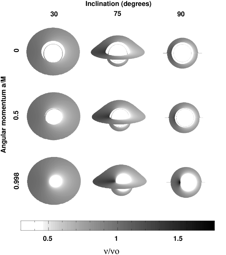
Figure 4: Images of the accretion disk observed in the iron-line by a distant observer. The top row of images is for a Schwarzschild black hole ($a_{\ast}=0$). The middle row shows the images for a Kerr black hole with $a_{\ast}=0.5$. The bottom row corresponds to an extreme Kerr hole ($a_{\ast}=0.998$). For each value of $a_{\ast}$, the image is shown for inclination angles $30^{\circ},75^{\circ}$ and $90^{\circ}$. The grey-scale indicates the variation of redshift in the image.

The fluorescent line is emitted with intensity $I_{\mbox{\scriptsize em}}(\nu_{\mbox{\scriptsize em}})$ in the local rest frame of the disk, and received with intensity $I_{\mbox{\scriptsize obs}}(\nu_{\mbox{\scriptsize obs}})$ by the distant observer. These intensities are related by the invariant along the photon path

$${I_{\mbox{\scriptsize obs}}(\nu_{\mbox{\scriptsize obs}})\over\nu_{\mbox{\scriptsize obs}}^{3}}={I_{\mbox{\scriptsize em}}(\nu_{\mbox{\scriptsize em}})\over\nu_{\mbox{\scriptsize em}}^{3}}.$$ (3.10)

We may then integrate over the solid angle subtended at the observer, and the frequency bins of the detector to obtain the flux. The emitted intensity $I_{\mbox{\scriptsize em}}(\nu_{\mbox{\scriptsize em}})$ will be a function of the radius of emission in the accretion disk. Typical assumptions are that the disk continuum emissivity follows $\epsilon(r)\propto r^{-q}$ with $q$ in the range 2–3, or that $\epsilon(r)$ follows the (more realistic) law of Page and Thorne $\mskip-3.0mu{}^{{\bf?}{}{LaTeXWarning:Citation`page74^{\prime}onpage0undefined}}$. We make the assumption that the line emissivity follows the latter, with emission starting at the radius of marginal stability. In Figure LABEL:fig-pred-lineprofs we show nine predicted line profiles for different values of $a_{\ast}$ and inclination angle. These suggest that for fixed emissivity profile, the overall line shape is most sensitive to the inclination angle. For sufficiently large inclination angles the spectrum is double peaked. This effect is mainly due to Doppler shifts between the receding and approaching parts of the disk $\mskip-3.0mu{}^{{\bf?}{}{LaTeXWarning:Citation`youri96^{\prime}onpage0undefined}}$. The two-parameter ($a_{\ast}$ and $i$) predicted lineshapes may now be fitted to the observed profile over the period of lowest luminosity. The $\chi^{2}$ confidence contours in the parameter space are shown in Figure LABEL:fig-chi along with the best-fit to the observed line flux. The $\chi^{2}$ contours give relatively strong evidence for an inclination angle of $\sim 25^{\circ}$ – $30^{\circ}$, and strongly favour an extreme Kerr black hole ($a_{\ast}>0.94$).

Figure 5: Calculated iron-line profiles as measured by the distant observer. The top row is for $a_{\ast}=0.998$, the middle row has $a_{\ast}=0.5$, and the bottom row is for a Schwarzschild black-hole $(a_{\ast}=0)$. For each value of angular momentum, line profiles are given for inclination angles of $0^{\circ},30^{\circ}$ and $89^{\circ}$.

Figure 6: Figure 6a shows the contours of probability versus $i$ and $a_{\ast}$, calculated assuming a uniform prior on each parameter. Figure 6b compares the calculated line flux (dashed line) corresponding to the best-fit values $i={29^{\circ}}^{+2.5}_{-3.2}$, $a_{\ast}=1^{+0}_{-0.01}$ with the observed data (marked points). The error bounds on the best-fit parameters are $68\%$ confidence intervals obtained by marginalization over the other parameter.

The need for a high value of $a_{\ast}$ is so crucial to fitting the observed line profile, that the observed line strongly constrains the emissivity profile $\epsilon(r)$. This allows us to infer an emissivity profile for the first time. We have done this with the other parameters $a_{\ast}$ and $i$ held fixed at the values 0.998 and $30^{\circ}$. The inferred profile is shown in Figure LABEL:fig-inf-prof. There is some evidence for a power law, with a value of $q\sim 3.5$, although it obviously becomes noisy at low flux levels.

Figure 7: A log-log plot of the inferred emissivity profile, for $a_{\ast}=0.998$ and inclination angle $i=30^{\circ}$.

4 The Nature of the Kerr Singularity

The problem we now wish to address concerns the endpoint of rotating collapsing matter. In the previous section we assumed that the collapsed system at the centre of the AGN was a Kerr black hole. For this reason it is of interest to look at the nature of the singularity inside a Kerr black hole, and so determine whether it is consistent with what we would expect for the end point of such a collapse. This problem was considered in Doran $\mskip-3.0mu{}^{{\bf?}{}{LaTeXWarning:Citation`DGL96-KSI^{\prime}onpage0undefined}}$ and Doran et al. $\mskip-3.0mu{}^{{\bf?}{}{LaTeXWarning:Citation`DGL96-KSII^{\prime}onpage0undefined}}$.

Gauge-theory gravity allows an unambiguous answer to this problem, provided that one accepts the basic premises of our theory. This is because the topological constraints implied by the theory ensure that we have well defined surfaces over which we may apply integral theorems. The results of this investigation will be a gauge invariant description of the nature of the singularity, but so far we have found that the problem is most tractable with a specific choice of gauge. We shall employ the ‘Kerr-Schild’ gauge, in which the $\overline{h}$-function takes the form

$$\overline{h}(a)=a+a{\cdot}ll,{}$$ (4.1)

where $l$ is a null vector ($l^{2}=0$). This $\overline{h}$-function is globally valid, unlike the gauge employed in the previous section. This is essential to study the nature of the singularity, since this lies inside the horizon. A simple example of a solution in the Kerr-Schild form is provided by a Schwarzschild black hole, which has

$$l=\sqrt{M/r}(\gamma_{0}-e_{r}).{}$$ (4.2)

In this gauge, incoming radial photons follow straight lines in a $(t,r)$ plot, and terminate on the singularity at $r=0$. Outgoing radial photons may only escape from the black hole if they start outside the horizon (which lies at $r=2M$). This solution is geodesically incomplete and is not time-reverse symmetric. This forces us to adopt the picture of the black hole being the end-point of a collapse process, with the formation of the horizon capturing information about the direction of time for which the collapse occurred $\mskip-3.0mu{}^{{\bf?}{}{LaTeXWarning:Citation`DGL-erice^{\prime}onpage0undefined},{\bf?}{}{LaTeXWarning:Citation`DGL-grav^{\prime}onpage0undefined}}$

It is easy to show that for a general Kerr-Schild vacuum solution $\mskip-3.0mu{}^{{\bf?}{}{LaTeXWarning:Citation`DGL96-KSI^{\prime}onpage0undefined}}$,

$$l{\cdot}\nabla l\propto l.$$ (4.3)

We shall only consider matter fields for which this relation is also true (this clearly restricts the matter fields that we may describe, but does include the Reissner-Nordstrom and Vaidya ‘shining star’ solutions). It follows that we may write

$$l{\cdot}\nabla l=\phi l,$$ (4.4)

where $\phi$ is an arbitrary scalar function of position. The Einstein tensor then takes the form

$${\mathcal{G}}(a)=\nabla{\cdot}[\Omega(a)-a{\wedge}(\gamma^{\mu}{\cdot}\Omega(\gamma_{\mu}))],{}$$ (4.5)

where

$$\omega(a)=\nabla{\wedge}(a{\cdot}ll)$$ (4.6)

and the vector $a$ is not differentiated. Equation (LABEL:eins) shows that for this class of fields, the Einstein tensor is a total divergence in the background spacetime. For stationary fields, it follows that the Einstein tensor is a total 3-divergence. This allows us to convert integrals of ${\mathcal{G}}(a)$ over the singular regions of space to surface integrals over well defined 2-surfaces enclosing the singularity.

For example, the Schwarzschild black hole (LABEL:schwarz) gives

$$\intop\nolimits_{r\leq r_{0}}d^{3}x\mskip 3.0mu{\mathcal{G}}(a)=8\pi Ma{\cdot}\gamma_{0}\gamma_{0},$$ (4.7)

where $r_{0}$ is any value $>0$, since ${\mathcal{G}}(a)$ vanishes everywhere except at the origin. It follows that the matter stress-energy tensor is given by

$${\mathcal{T}}(a)=M\delta(\mbox{\boldmath$x$})a{\cdot}\gamma_{0}\gamma_{0},$$ (4.8)

where $\mbox{\boldmath$x$}\equiv x{\wedge}\gamma_{0}$. This is the stress-energy tensor appropriate to a point source of matter (of mass $M$) following the world line $r=0$. This technique is analogous to the usual analysis of the singularity in the Coulomb field, due to a point charge. Note that the integrals that we have performed are not gauge invariant, but we have extracted gauge covariant information in the form of the stress-energy tensor.

4.1 The Reissner-Nordstrom solution

We now highlight a result obtained by one of us in Doran $\mskip-3.0mu{}^{{\bf?}{}{LaTeXWarning:Citation`DGL96-KSI^{\prime}onpage0undefined}}$. The Reissner-Nordstrom solution describes a charged, non-rotating black hole. In the Kerr-Schild gauge, the solution may be written in the form

$$\overline{h}(a)=a+\eta a{\cdot}e_{-}e_{-},$$ (4.9)

where,

$$\eta\equiv{M\over r}-{q^{2}\over 8\pi r^{2}},\qquad e_{-}\equiv\gamma_{0}-e_{r},$$ (4.10)

and $q$ is the charge of the source. Away from the origin, the stress-energy tensor evaluates to

$${\mathcal{T}}(a)=-{\textstyle{1\over 2}}{\mathcal{F}}a{\mathcal{F}},$$ (4.11)

where ${\mathcal{F}}\equiv qe_{r}\gamma_{0}/(4\pi r^{2})$. This is the expected form for the electromagnetic stress tensor due to a point charge $q$ at the origin. To study the behaviour in the singular region, we return to equation (LABEL:eins) to obtain

$$\intop\nolimits_{r\leq r_{0}}d^{3}x\mskip 3.0mu{\mathcal{T}}(a)=Ma{\cdot}\gamma_{0}\gamma_{0}+{q^{2}\over 24\pi r_{0}}(a-4a{\cdot}\gamma_{0}\gamma_{0}).$$ (4.12)

The first term on the right-hand side is the same as in the Schwarzschild case, whilst the latter is the trace-free electromagnetic contribution. Concentrating on the $\gamma_{0}$-frame energy component, we find that

$$\intop\nolimits_{r\leq r_{0}}d^{3}x\mskip 3.0mu\gamma_{0}{\cdot}{\mathcal{T}}(\gamma_{0})=M-{q^{2}\over 8\pi r_{0}}.$$ (4.13)

Something remarkable has happened here — due to the gravitational fields,, the electromagnetic contribution to the energy is now negative and vanishes as we extend the integral over all of space ($r_{0}\rightarrow\infty$). This is in stark contrast to the standard picture from classical electromagnetism, where the self-energy of the point charge diverges. Inclusion of the gravitational fields has removed this divergence, ensuring that the total electromagnetic self-energy vanishes. The manner in which this regularisation is achieved is discussed in Doran $\mskip-3.0mu{}^{{\bf?}{}{LaTeXWarning:Citation`DGL96-KSI^{\prime}onpage0undefined}}$.

4.2 The Kerr solution

The Kerr solution describes a rotating, uncharged black hole. A remarkable complex harmonic structure underlying this solution was found by Schiffer et al. $\mskip-3.0mu{}^{{\bf?}{}{LaTeXWarning:Citation`sch73a^{\prime}onpage0undefined}}$. We define ‘complex’ numbers $\gamma$ and $\omega$ via

$$\gamma\equiv\alpha+i\beta,\qquad\omega\equiv\gamma^{-1},{}$$ (4.14)

where $\alpha$ and $\beta$ are scalars. Not that the ‘$i$’ appearing in equation (LABEL:comp) is the spacetime pseudoscalar. This element is the generator of duality transformations. For example, the STA statement of the self-duality of the Weyl tensor is

$${\mathcal{W}}(iB)=i{\mathcal{W}}(B),$$ (4.15)

where $B$ is an arbitrary bivector. We obtain an axisymmetric solution of Kerr-Schild form if we can solve the two equations

$$\mbox{\boldmath$\nabla$}^{2}\gamma=0,\qquad(\mbox{\boldmath$\nabla$}\omega)^{2}=1,$$ (4.16)

where $\mbox{\boldmath$\nabla$}\equiv\gamma_{0}{\wedge}\nabla$ is the derivative operator in the space orthogonal to $\gamma_{0}$. Any solution of these equations generates a Kerr-Schild type solution of the form (LABEL:kerrhfunc), with $l$ given in terms of $\gamma$ and $\gamma_{0}$ $\mskip-3.0mu{}^{{\bf?}{}{LaTeXWarning:Citation`DGL96-KSII^{\prime}onpage0undefined}}$.

As a simple example, the Schwarzschild solution is obtained by setting $\omega=r$. We can obtain the Kerr solution by a ‘complex translation’ of the Schwarzschild solution:

$$\omega=(x^{2}+y^{2}+(z-iL)^{2})^{1/2},$$ (4.17)

where $L$ is a scalar constant, and $\{x,y,z\}$ are Cartesian coordinates. The Riemann tensor for this solution evaluates to

$${\mathcal{R}}(B)=-{M\over 2\omega^{3}}(B+3\sigma_{\gamma}B\sigma_{\gamma}),$$ (4.18)

with the unit bivector $\sigma_{\gamma}$ given by

$$\sigma_{\gamma}\equiv{\mbox{\boldmath$x$}-Li\sigma_{3}\over\omega}.$$ (4.19)

The Riemann tensor is only singular where $\omega=0$ which occurs on the ring $\rho=L,z=0$ ($\rho\equiv(x^{2}+y^{2})^{1/2}$). For this reason, it has been widely believed that the Kerr singularity is a ring only.

We can analyse the nature of the Kerr singularity in a similar manner to the Schwarzschild and Reissner-Nordstrom cases treated earlier. We begin by integrating over a spatial region which fully encloses the central disk. We find that

$$\intop\nolimits d^{3}x\mskip 3.0mu{\mathcal{T}}(a)=Ma{\cdot}\gamma_{0}\gamma_{0},$$ (4.20)

where $M$ is the mass of the hole (this constant appears when relating $\omega$ to $l$), and the integral is taken over any region enclosing the central disk. This is the same result as in the Schwarzschild case. We can also integrate the (orbital) angular momentum tensor $x{\wedge}{\mathcal{T}}(a)$ ($x$ being the spacetime position vector) over the region enclosing the disk to obtain

$$\intop\nolimits d^{3}x\mskip 3.0mux{\wedge}{\mathcal{T}}(a)=ML[-a{\cdot}\gamma_{0}i\sigma_{3}+{\textstyle{1\over 2}}(a{\wedge}\gamma_{0}){\times}i\sigma_{3}].$$ (4.21)

This clearly identifies $ML$ as the total angular momentum in the fields, as expected from their long-range behaviour.

To examine the matter distribution for $\rho\leq L$, we integrate the Einstein tensor over cylindrical 3-volumes normal to the disk. The calculations are lengthy and great care must be taken over the choice of branch for the complex square roots. Details are given in Doran et al. $\mskip-3.0mu{}^{{\bf?}{}{LaTeXWarning:Citation`DGL96-KSII^{\prime}onpage0undefined}}$, where it is shown that for $\rho<L$,

 

$${{\mathcal{G}}(\gamma_{0})}$$

(4.22)

The vectors $e_{\rho}$ and $\mathaccent 28766{\phi}$ are unit spacelike basis vectors in the cylindrical polar coordinate system. This form for the Einstein tensor clearly shows that matter is not located solely on the ring at $\rho=L$, but also over a disk in the plane $z=0$, which has the ring as its boundary. We see immediately that ${\mathcal{T}}(a)$ is symmetric, showing that there are no hidden sources of torsion in the disk. This contribution to the Einstein tensor describes a rigidly-rotating, massless disk of pure isotropic tension in the plane of the disk. The tension is given by $M/[4\pi L(L^{2}-\rho^{2})^{1/2}]$. The angular velocity is $1/L$ so that the edge of the disk follows a lightlike trajectory. Remarkably, this tension field has a simple non-gravitational explanation. The special-relativistic equations governing a massless, rigidly-rotating membrane (with a ring of particles attached to the edge) reproduce exactly the functional form with $\rho$ just found for this tension. The fact that the disk has vanishing energy density but generates a tension means that it violates the weak energy condition.

The integral of the Ricci scalar over the interior of the disk yields $8\pi M$, which is equal to the value deduced from integrals enclosing the entire singular region. It follows that any matter in the ring at $\rho=L$ makes no contribution to the Ricci scalar, and hence that the contribution to the stress-energy tensor from the ring singularity must have vanishing trace. Furthermore, the disk of pure isotropic tension can make no contribution to the angular momentum of the fields, so the angular momentum must come solely from the ring singularity. From these considerations, we may deduce that the matter in the ring follows a lightlike trajectory. These conclusions are gauge invariant, since they are inferred from the eigenvalue structure of covariant tensors.

We see that within the framework of gauge-theory gravity, the Kerr singularity is composed of a ring of matter, moving at the speed of light, which surrounds a disk of pure isotropic tension. The tension in this disk has precisely the form expected on the basis of special-relativistic arguments. The rotating ring of matter is a perfectly satisfactory endpoint for matter collapsing with angular momentum — the proper radius coincides with the minimum size allowed by special relativity, for an object with angular momentum $ML$. However, the presence of the disk of tension is problematic — no baryonic matter can have a tension but vanishing energy density. If baryonic matter cannot form this disk, then what is the status of the Kerr solution as the endpoint of the collapse process? The answer to this question must await the discussion of realistic collapse processes within the framework of gauge-theory gravity.

5 Rigidly-Rotating Cosmic Strings

As a final topic, we shall turn to a situation with cylindrical symmetry. We shall restrict attention to string solutions in which the direction along the string axis plays no part in the dynamics of the string. Imposing this restriction means that the solutions which include pressure will violate the boost invariance, which is usually demanded of all cosmic string solutions. However, these solutions may still be of use for rotating strings in (3+1)-dimensions, where it is not clear that one can impose boost invariance.

We adopt a cylindrical polar coordinate system $\{t,\rho,\phi,z\}$:

 

$${t}$$

(5.1)

The vectors $\{e_{t},e_{\rho},e_{\phi},e_{z}\}$ comprise the associated coordinate frame, with $e_{t}\equiv\gamma_{0}$ and $e_{z}\equiv\gamma_{3}$. The reciprocal frame vectors are denoted as $\{e^{t},e^{\rho},e^{\phi},e^{z}\}$. We shall consider solutions described by an $\overline{h}$-function of the form

 

$${\overline{h}(e^{t})}$$

(5.2)

We require that the $\overline{h}$-function (and the $\Omega$-function) be well defined on the string axis ($z=0$). This requires that $f_{2},\rho h_{1}$ and $h_{2}$ all vanish smoothly on the axis. These requirements replace the notion of ‘elementary flatness’ employed in the general relativity literature $\mskip-3.0mu{}^{{\bf?}{}{LaTeXWarning:Citation`syn-gr^{\prime}onpage0undefined}}$. This is an area where gauge-theory gravity offers clear advantages over general relativity — since we deal solely with linear functions defined over a (flat) background spacetime, there is never any doubt about the conditions that these functions should satisfy.

5.1 The solution of Jensen and Soleng

The first published solution describing the interior of a finite width rotating string was that of Jensen and Soleng $\mskip-3.0mu{}^{{\bf?}{}{LaTeXWarning:Citation`jen92^{\prime}onpage0undefined}}$. Their solution may be generated from an $\overline{h}$-function of the form (LABEL:hfunc-string) with

 

$${h_{1}}$$

(5.3)

where

$$A={1\over\sqrt{\lambda}}\mathop{\kern 0.0pt\symoperators sin}\nolimits(\sqrt{\lambda}\rho),$$ (5.4)

and

$$M=2\alpha\left((\rho-\rho_{s})\mathop{\kern 0.0pt\symoperators cos}\nolimits(\sqrt{\lambda}\rho)-{1\over\sqrt{\lambda}}\mathop{\kern 0.0pt\symoperators sin}\nolimits(\sqrt{\lambda}\rho)+\rho_{s}\right).$$ (5.5)

Here $\lambda$ is a positive constant, $\alpha$ is a constant with $\alpha\leq 1$, and $\rho_{s}$ is the radius of the string. The parameter $u$ appearing in (LABEL:hfunc-jen) is arbitrary up to the constraint that $u=0$ on the axis of the string (so that the $\overline{h}$-function is well defined there). Analysing the solution in the gauge in which $u=0$ everywhere, we find that

$${\mathcal{G}}(e_{t})=-\alpha_{2}e_{t}+\alpha\lambda\mathaccent 28766{\phi},$$ (5.6)

where $\alpha_{2}$ is a function whose explicit from we do not require. The vector $\mathaccent 28766{\phi}$ is given by

$$\mathaccent 28766{\phi}\equiv e_{\phi}/\rho=-\mathop{\kern 0.0pt\symoperators sin}\nolimits\mskip-3.0mu\phi\gamma_{1}+\mathop{\kern 0.0pt\symoperators cos}\nolimits\mskip-3.0mu\phi\gamma_{2}.$$ (5.7)

If we now consider an observer with covariant velocity $e_{t}$ passing through the axis of the string, it is clear that the 3-momentum density he measures on the axis is ill-defined.

The conclusion is that the solution of Jensen and Soleng does not define a physically acceptable matter distribution. This is surprising, since the solution does satisfy the criteria of elementary flatness. This point illustrates a further advantage of the gauge theory approach over general relativity; the gauge theory focuses attention on the physically relevant quantities, such as the eigenvalues of the stress-energy tensor. In such an approach, it quickly becomes apparent if a solution has unphysical properties.

5.2 Rigidly-rotating strings

It is not difficult to find rotating string solutions with a physically acceptable matter distribution. The simplest model is that of a two dimensional ideal fluid, with stress-energy tensor

 

$${{\mathcal{T}}(e_{t})}$$

(5.8)

The covariant 4-velocity of the fluid is $e_{t}$, the energy density is $\mu(\rho)$ and the isotropic pressure in the $i\sigma_{3}$ plane is $p(\rho)$. The coefficient of ${\mathcal{G}}(e_{z})$ is restricted to $\mu-2p$ by the Einstein equations, and the assumed form for the $\overline{h}$-function (LABEL:hfunc-string). This stress-energy tensor is well defined on the axis, provided that the pressure and energy density are finite there.

A rigidly-rotating (shear-free) solution is given by

 

$${h_{1}}$$

(5.9)

where $\lambda$ is an arbitrary positive constant, and the constant $A$ satisfies $A<-1$. It is simple to show that this linear function is well defined on the axis. The pressure and energy density evaluate to

$$\openup 3.0pt\halign to=0.0pt{\ifst@rred\nonumber\fi\hfil\strut@\setboxz@h{\global\tag@false$\m@th\displaystyle{\@lign#}$}\global\lwidth@\wdz@\boxz@\global\advance\and@\@ne&\setboxz@h{$\m@th\displaystyle{{}\@lign#}$}\global\rwidth@\wdz@\boxz@\hfill\global\advance\and@\@ne&\setboxz@h{\@lign\strut@{#}}\dimen@\displaywidth\advance\dimen@-\totwidth@\divide\dimen@\tw@\advance\dimen@\maxrwidth@\advance\dimen@-\rwidth@\ifdim\dimen@<\tw@\wdz@\llap{\vtop{\@movetag\normalbaselines\null\boxz@}}\else\llap{\boxz@}\fi\cr\hbox{$\displaystyle{8\pi p&\hbox{$\displaystyle{{}=K^{2}-GT{}&\hbox to0.0pt{\hss\vtop{\hbox{}\hbox{{\hbox{(\ignorespaces 5.10)\cr\vskip 0.0pt\cr\hbox{$\displaystyle{8\pi\mu&\hbox{$\displaystyle{{}=3K^{2}+\lambda^{2},&\hbox to0.0pt{\hss\vtop{\hbox{}\hbox{{\hbox{(\ignorespaces 5.11)\cr\nointerlineskip\vskip 0.0pt\vskip 0.0pt\vbox{\noindent\hbox to65.70074pt{\hfill}}\cr}}}}}}}}}}}}}}}}}}}$$

where the functions $G,K$ and $T$ are given by

$$G={\lambda\mathop{\kern 0.0pt\symoperators cos}\nolimits\mskip-3.0mu\lambda\rho\over\mathop{\kern 0.0pt\symoperators sin}\nolimits\mskip-3.0mu\lambda\rho}\qquad K={B\over(A+\mathop{\kern 0.0pt\symoperators cos}\nolimits\mskip-3.0mu\lambda\rho)^{2}}\qquad T={\lambda\mathop{\kern 0.0pt\symoperators sin}\nolimits\mskip-3.0mu\lambda\rho\over A+\mathop{\kern 0.0pt\symoperators cos}\nolimits\mskip-3.0mu\lambda\rho},$$ (5.12)

with $B$ a further constant. The functions $G,K$ and $T$ arise naturally in the rotation-gauge field. The boundary of the string occurs where $p=0$, and this must be reached before $\rho>\pi/\lambda$.

This interior solution matches onto the exterior vacuum solution given by

$$\openup 3.0pt\halign to=0.0pt{\ifst@rred\nonumber\fi\hfil\strut@\setboxz@h{\global\tag@false$\m@th\displaystyle{\@lign#}$}\global\lwidth@\wdz@\boxz@\global\advance\and@\@ne&\setboxz@h{$\m@th\displaystyle{{}\@lign#}$}\global\rwidth@\wdz@\boxz@\hfill\global\advance\and@\@ne&\setboxz@h{\@lign\strut@{#}}\dimen@\displaywidth\advance\dimen@-\totwidth@\divide\dimen@\tw@\advance\dimen@\maxrwidth@\advance\dimen@-\rwidth@\ifdim\dimen@<\tw@\wdz@\llap{\vtop{\@movetag\normalbaselines\null\boxz@}}\else\llap{\boxz@}\fi\cr\hbox{$\displaystyle{f_{1}&\hbox{$\displaystyle{{}=-(1+A)(\alpha/B)^{1/2}[(\rho+\rho_{0})^{2}-\alpha^{2}]^{-1/2}{}&\hbox to0.0pt{\hss\vtop{\hbox{}\hbox{{\hbox{(\ignorespaces 5.13)\cr\vskip 0.0pt\cr\hbox{$\displaystyle{h_{1}&\hbox{$\displaystyle{{}=(\alpha/B)^{1/2}\lambda^{2}{[(\rho+\rho_{0})^{2}-\alpha^{2}]^{1/2}\over(\rho+\rho_{0})}{}&\hbox to0.0pt{\hss\vtop{\hbox{}\hbox{{\hbox{(\ignorespaces 5.14)\cr\vskip 0.0pt\cr\hbox{$\displaystyle{f_{2}&\hbox{$\displaystyle{{}={\alpha\over f_{1}(\rho+\rho_{0})}({f_{1}}^{2}-1){}&\hbox to0.0pt{\hss\vtop{\hbox{}\hbox{{\hbox{(\ignorespaces 5.15)\cr\vskip 0.0pt\cr\hbox{$\displaystyle{h_{2}&\hbox{$\displaystyle{{}=0.&\hbox to0.0pt{\hss\hbox{{\hbox{(\ignorespaces 5.16)\cr\nointerlineskip\vskip 0.0pt\vskip 0.0pt\vbox{\noindent\hbox to161.2265pt{\hfill}}\cr}}}}}}}}}}}}}}}}}}}}}}}}}}}}}}}}}}}}$$

The constants $\rho_{0}$ and $\alpha$ must be determined by the matching conditions at the string boundary. This class of vacuum solution does not appear to correspond to anything given previously in the literature. There is a confining force in the vacuum meaning that no particle can escape from the string, regardless of the initial velocity that it is given.

The line element associated with this external solution is

$$\openup 3.0pt\halign{\Let@\let\tag\gobble@tag\hbox to\totwidth@{\strut@$\m@th\displaystyle\if@fleqn\hskip 0pt plus 1000pt \else\hfil\fi{}#\hfil$}\cr.0pt{$\displaystyle\hfil{}\hfilneg\hskip 10.0ptds^{2}={B\over\alpha(1+A)^{2}}\bigl{(}(\rho+\rho_{0})^{2}-\alpha^{2}\bigr{)}\mskip 3.0mudt^{2}-{B^{2}(\rho+\rho_{0})^{2}\over(1+A)^{2}\alpha^{2}\lambda^{4}}\bigl{(}{f_{1}}^{2}-{f_{2}}^{2}\bigr{)}\mskip 3.0mud\phi^{2}{}\cr\vskip 0.0pt\cr.0pt{$\displaystyle\hfil{}+{2B\over\lambda^{2}(A+1)}\Bigl{(}1-{B\over\alpha(1+A)^{2}}\bigl{(}(\rho+\rho_{0})^{2}-\alpha^{2}\bigr{)}\Bigr{)}\mskip 3.0mudt\mskip 3.0mud\phi-d\rho^{2}-dz^{2}.\hskip 10.0pt\hbox to0.0pt{\hss\vtop{\hbox{}\hbox{\hbox{\hbox{(\ignorespaces 5.17)}}}}}\hfilneg\crcr}}}$$

This class of rigidly-rotating strings is of particular interest because these solutions always admit closed timelike curves at some distance from the string. This follows from the fact that for large $\rho$, $f_{1}$ varies as $1/\rho$ whereas $f_{2}$ tends to a constant value. Beyond the point where the magnitude of $f_{2}$ exceeds that of $f_{1}$, a closed circular path around the string becomes timelike. The long-range properties of these solutions make them ultimately unphysical, but there is no reason to suppose that the solutions will not be relevant near a string of finite length.

References

References

- [1] R. Utiyama. Invariant theoretical interpretation of interaction. Phys. Rev., 101(5):1597, 1956.
- [2] T.W.B. Kibble. Lorentz invariance and the gravitational field. J. Math. Phys., 2(3):212, 1961.
- [3] A.N. Lasenby, C.J.L. Doran, and S.F. Gull. Astrophysical and cosmological consequences of a gauge theory of gravity. In N. Sánchez and A. Zichichi, editors, Advances in Astrofundamental Physics, Erice 1994, page 359. World Scientific, Singapore, 1995.
- [4] A.N. Lasenby, C.J.L. Doran, and S.F. Gull. Gravity, gauge theories and geometric algebra. To appear in Phil. Trans. R. Soc. Lond. A, 1996.
- [5] Y. Tanaka, K. Nandra, A.C. Fabian, H. Inoue, C. Otani, T. Dotani, K. Hayashida, K. Iwasawa, T. Kii, H. Kunieda, F. Makino, and M. Matsuoka. Gravitationally redshifted emission implying an accretion disk and massive black-hole in the active galaxy MCG-6-30-15. Nature, 375:659, 1995.
- [6] K. Iwasawa, A.C. Fabian, C.S. Reynolds, K. Nandra, C. Otani, H. Inoue, K. Hayashida, W.N. Brandt, T. Dotani, H. Kunieda, M. Matsuoka, and Y. Tanaka. The variable iron K emission line in MCG-6-30-15. Mon. Not. R. Astron. Soc., 283:1038, 1996.
- [7] C.J.L. Doran. Integral equations and Kerr-Schild fields I. Spherically-symmetric fields. Submitted to: Class. Quantum Grav., 1996.
- [8] C.J.L Doran, A.N. Lasenby, and S.F Gull. Integral equations and Kerr-Schild fields II. The Kerr solution. Submitted to: Class. Quantum Grav., 1996.
- [9] C.J.L. Doran, A.N. Lasenby, and S.F. Gull. The physics of rotating cylindrical strings. To appear in: Phys. Rev. D, 1996.
- [10] B. Jensen and H.H. Soleng. General-relativistic model of a spinning cosmic string. Phys. Rev. D, 45(10):3528, 1992.
- [11] D. Hestenes. Space-Time Algebra. Gordon and Breach, New York, 1966.
- [12] A.D. Challinor, A.N. Lasenby, C.J.L. Doran, and S.F. Gull. Massive, non-ghost solutions for the self-consistent Dirac field. In preparation, 1996.
- [13] K.A. Pounds, K. Nandra, G.C. Stewart, I.M. George, and A.C. Fabian. X-ray reflection from cold matter in the nuclei of active galaxies. Nature, 344:132, 1990.
- [14] M. Matsuoka, L. Piro, M. Yamauchi, and T. Murakami. X-ray spectral variability and complex absorption in the Seyfert-1 galaxies NGC-4051 and MCG-6-30-15. ApJ, 361:440, 1990.
- [15] A. Laor. Line-profiles from a disk around a rotating black-hole. ApJ, 376:90, 1991.
- [16] Y. Kojima. The effects of black-hole rotation on line-profiles from accretion disks. Mon. Not. R. Astron. Soc., 250:629, 1991.
- [17] Y. Dabrowski, A.C. Fabian, K. Iwasawa, A.N. Lasenby, and C.S. Reynolds. The profile and equivalent width of the X-ray iron emission-line from a disk around a Kerr black hole. Submitted to Mon. Not. R. Asron. Soc., 1996.
- [18] D. Hestenes. Proper dynamics of a rigid point particle. J. Math. Phys., 15(10):1778, 1974.
- [19] K.S. Thorne. Disk-accretion onto a black hole II. Evolution of the hole. ApJ, 191:507, 1974.
- [20] C.W. Misner, K.S. Thorne, and J.A. Wheeler. Gravitation. W.H. Freeman and Company, San Francisco, 1973.
- [21] D.N. Page and K.S. Thorne. Disk-accretion onto a black hole I. Time averaged structure of accretion disk. ApJ, 191:499, 1974.
- [22] M.M. Schiffer, R.J. Adler, J. Mark, and C. Sheffield. Kerr geometry as complexified Schwarzschild geometry. J. Math. Phys., 14:52, 1973.
- [23] J.L. Synge. Relativity: The General Theory. North-Holland Publishing, Amsterdam, 1964.