The Stellar Distribution of the Globular Cluster M55

Abstract

We have used extensive $V$, $I$ photometry (down to $V=20.9$) of $33615$ stars in the direction of the globular cluster M55 to study the dynamical interaction of this cluster with the tidal fields of the Galaxy. An entire quadrant of the cluster has been covered, out to $\simeq 1.5$ times the tidal radius.

A CMD down to about 4 magnitudes below the turn-off is presented and analysed. A large population of BS has been identified. The BS are significantly more concentrated than the other cluster stars in the inner 300 arcsec, while they become less concentrated in the cluster envelope.

We have obtained luminosity functions at various radial intervals from the center and their corresponding mass functions. Both clearly show the presence of mass segregation inside the cluster. A dynamical analysis shows that the observed mass segregation is compatible with what is predicted by multi-mass King-Michie models. The global mass function is very flat with a power-law slope of $x=-1.0\pm 0.4$. This suggest that M55 might have suffered selective losses of stars, caused by tidal interactions with the Galactic disk and bulge.

The radial density profile of M55 out to $\sim 2\times r_{t}$ suggests the presence of extra-tidal stars whose nature could be connected with the cluster.

1 Introduction

The recent advances in our understanding of the structure and evolution of Galactic globular clusters (GCs) have been possible thanks to the advent of accurate CCD photometry. However, till few years ago, CCD photometry was limited to the internal parts of GCs due to the small fields of the detectors. All the information relative to the outer regions and to the tidal radius $r_{t}$, arise from visual (by eye) stellar counts made on Schmidt plates, especially by King and collaborators King et al. (1968); Trager et al. (1995). This methodology of investigation suffers from various problems and statistical biases; we list some of them:

• The limiting magnitude of photographic plates, which is generally too bright to permit the investigation of the radial distribution of stars in an appropriate mass range;

• the high uncertainty in the evaluation of background stellar contamination;

• an insufficient crowding/completeness correction.

All the more recent models of dynamical evolution need to make assumptions on the mass function, on the effects due to the radial anisotropy of the velocity distribution, and on the mass segregation which, in principle, could be determined observationally.

Figure 1: EMMI fields coverage of M55. The center of the cluster is inside field number 1. The circles mark the approximate position of: one core radius, $1r_{c}$, two core radii, $2r_{c}$, and the tidal radius, $r_{t}$.

Fostered by this lack of observational data, five years ago we started a long term project using one of the largest field CCD cameras available, EMMI at the NTT, to obtain accurate stellar photometry in two bands, $V$ and $I$, over at least a full quadrant in a number of GCs. The sample was selected taking into account the different morphological types and the different positions in the Galaxy. The principal aim was to map the stellar distribution from the central part out to the outer envelope (beyond the formal tidal radius, for a better estimate of the field stars contamination and in order to investigate on the possible presence of tidal tails), with a good statistical sampling of the stars in distinct zones of the color magnitude diagram (CMD) and of different masses.

The use of CCD star counts, instead of photographic Schmidt plates for which the only advantage is still to give a larger area coverage (Grillmair et al., 1995; Lehman & Sholz, 1997, for works on this subject), allows us to go deeper inside the core of the clusters, to better handle photometric errors and completeness corrections and to reach a considerably fainter magnitude level. CCDs also allows in the case of high concentration clusters to complement star counts of the central part with aperture photometry of short exposures images Saviane et al. (1997).

An important byproduct of this study is the photometry of a significant number of stars in all the principal sectors of the CMD. This sample is of fundamental importance to test modern evolutionary stellar models Renzini & Fusi Pecci (1988). In all cases the CMD extends well below the turn off of the main sequence. This permits us to estimate the effect of mass segregation for masses from the TO mass ($\sim 0.8\mbox{$M_{\sun}$}$) down to $0.6,0.5\mbox{$M_{\sun}$}$.

So far, we have collected data for a total of 19 clusters. Same of them have already been reduced and analyzed. In this work we present the analysis of the star counts of the globular cluster NGC 6809=M55. Other clusters, for which we have already given a first report elsewhere Zaggia et al. (1995); Veronesi et al. (1996); Saviane et al. (1995); Rosenberg et al. (1996), will be presented in future works Saviane et al. (1997); Rosenberg et al. (1997).

2 Why the globular cluster M55?

M55 is a low central concentration, $c=0.8$ Trager et al. (1995), low metallicity, ${\rm[Fe/H]}=-1.89$ Zinn (1980), cluster located at $\simeq 4.9$ kpc from the Sun Mandushev et al. (1996). Although it is a nearby object, it has received little or sporadic attention until very recently. The works of Mateo et al.. (1996) and Fahlman et al. (1996) presented photometric datasets of M55 that have been used principally to establish the age and the tidal extension of the Sagittarius dwarf galaxy. Mandushev et al. (1996) published the first deep (down to $V\simeq 24.5$) photometry of the cluster (other previous studies of the stellar population of M55 are in Lee, 1977; Shade, VandenBerg, and Hartwick, 1988; and Alcaino et al., 1992). From the data of a field at $\simeq 2$ core radii from the center, Mandushev et al. (1996) estimated a new apparent distance modulus for M55, $(m-M)_{V}=13.90\pm 0.09$, and from the luminosity function they found that the high-mass end of the mass function ($0.5<M/M_{\odot}<0.8$) is well fitted by a power law with $x=0.5\pm 0.2$, whereas at the low-mass end ($M/M_{\odot}<0.4$) the mass function has a slope of $x=1.6\pm 0.1$.

From the dynamical point of view, M55 has been previously studied by Pryor et al. (1991) in their papers on the mass-to-light ratio of globular clusters. Their principal conclusion is that this cluster might have a power law mass function with an exponent $x=1.35\div 2.0$, with a lower limit of the mass function in the range $\simeq 0.1\div 0.3\mbox{$M_{\sun}$}$ (i.e. a total absence of low mass stars): a conclusion opposite to that found recently by Mandushev et al. (1996).

Figure 2: Color magnitude diagram $Vvs.(V-I)$ for 33615 of M55.

An original work on M55 is in Irwin & Trimble (1984). They studied the radial star count density profile using photographic material digitalized with the Automatic Plate Measuring System (APM) of the Cambridge University. Irwin & Trimble (1984) used a single photometric band, which did not allow them to lower the contribution of the field stars in the construction of the radial star counts. Nevertheless in this work (never repeated in other clusters), the authors reach some interesting conclusions: they claim one of the first evidences of mass segregation (even if they cannot quantify it); the central stellar luminosity function seems to be flat (with a corresponding mass function having a slope of $x\simeq 0.0$) with a partial deviation from the King models. Moreover, they claim the presence of 8 short period variables, at the limit of their photometry, compatible with contact binaries of W UMa type. This last point is interesting for the presence of a large population of Blue Straggler (BS) stars in M55 to which the variables of Irwin & Trimble (1984) could belong.

Despite the potential interest of this nearby cluster for problems such as the dynamical evolution of globular clusters and interaction with the tidal field of the Galaxy, the existing data on M55 are so far limited and have been used to address only particular problems. Now large field CCDs offer the possibility to attack this problems in a suitable way. The following Section is dedicated to the presentation of the M55 data set and our observing strategy; in Section 4 we show the luminosity and mass function of the cluster; in Section 5 we present the analysis of the radial density profile and the conclusions. The details of the techniques adopted in the reduction and analysis of the data can be found in the appendix of the paper.

Figure 3: CMD $Vvs.(V-I)$ of M55 stars in three different radial intervals corresponding to $r\leq r_{c}$, $r_{c}<r\leq 2r_{c}$, and $r>2r_{c}$.

3 The photometric data

A whole quadrant of M55 was mapped (from the center out to $\sim 1.5\leavevmode\nobreak\ r_{t}$, with $r_{t}=977^{\prime\prime}$ as in Trager, King, and Djorgovski, 1995), on the night of July 5 1992 with 18 EMMI-NTT fields ($7\aas@@fstack{\prime}2\times 7\aas@@fstack{\prime}2$) in the $V$ and $I$ bands. Figure 1 shows the field positions on the sky. For each field a $V$ and a $I$ band image were taken in succession, with exposure times of 40 and 30 seconds respectively. The night was not photometric and the observing conditions improved as we moved from the outer fields to the internal ones. Information on the various fields and on all the technicalities of the reduction and analysis are reported in the appendix of the paper.

The $V$ vs. $(V-I)$ color magnitude diagram for a total of 33615 stars of M55 is shown in Figures 2 and 3. In total we detected 36800 objects of the cluster$+$field; $\simeq 9\%$ of them were eliminated after having applied a selection in the DAOPHOT II PSF interpolation parameters as in Piotto et al. (1990a). Although the exposure time was relatively short, the brightest stars of the red giant branch and of the asymptotic giant branch are saturated, though they can be still used for the radial star counts. We have omitted them from the final CMD.

In the following we will analyze the data using a division into three radial subsamples: inner ($r\leq r_{c}$), intermediate ($r_{c}<r\leq 2r_{c}$), and outer ($2r_{c}<r\leq r_{t}$). The core radius is $r_{c}=143\arcsec$, as found from the radial density profile analysis (cf. Section 5). In Figure 3 we show the brightest part of the CMD of M55, divided in the three radial subsamples. A large population of blue straggler stars (BS) is clearly visible, particularly in the inner part of the cluster where the background/foreground star contamination is low. In the intermediate zone, the BS population is better defined, and the sequence seems to reach brighter magnitudes. The BS sequence of the inner part appears to be broader in color than the sequence of the intermediate radial range. Part of this broadening can be attributed to the photometric errors that are larger in the inner region than in the intermediate one. The rest of the broadening is probably natural and could be connected to the two formation mechanisms of BS stars: the outer BS stars might mainly come from merger events, while the inner BS might be the final products of collisions (see Bailyn 1995).

Figure 4: Upper panel. Cumulative distribution of the SGB stars (solid line) and of BS stars (dashed line). Lower panel. Radial trend of the ratio of the number of BS stars ($N_{BS}$) and the number of SGB stars ($N_{SGB}$) in the same magnitude interval as the BS. Note the bimodal distribution.

We compared the distribution of the 95 BS with that of the 1669 sub-giant branch (SGB) stars selected in the same magnitude interval. In order to minimize the background star contamination along the SGB (very low indeed in the inner part of the cluster), we chose only the stars inside $\pm 2.0\sigma$ (where $\sigma$ is the standard deviation in the mean color) from the mean position of the SGB. We subtracted the background stellar contamination estimated from the star counts in the radial zone $r>1.1\leavevmode\nobreak\ r_{t}$. The BS seem to be more concentrated than the corresponding SGB stars only in the inner $250\div 300\arcsec$ (Figure 4). At larger distances, the BS distribution becomes less concentrated than the comparison SGB stars. We run a 2-population Kolmogorov-Smirnov test. The test does not give a particularly high statistical significance to the result: the probability that the BS and SGB stars are not taken from the the same distribution is 96%. However, this possibility cannot be excluded: see Piotto et al. (1990b) and Djorgovski & Piotto (1993) for a discussion on the limits in applying this statistical test for checking population gradients. Another way to look into the same problem is to investigate the radial trend of the ratio BS/SGB, as plotted in Figure 4 (lower panel). Also in this case the bimodal trend is quite evident. The relative number of BS stars decreases from the center of the cluster to reach a minimum at $r\simeq 250\div 300$ arcsec ($r\simeq 2r_{c}$), and then it rises again. Again, the statistical significance is questionable, in view of the small number of BS at $r>300$ arcsec (6 stars). Nevertheless, this possible bimodality is noteworthy. Indeed, there is a growing body of evidence that the radial distribution of BS stars in GCs might be bimodal, as shown by Ferraro et al. (1997) for M3 or Saviane et al. (1997) and Piotto et al. (1997) for NGC 1851. What makes our result for M55 of some interest is that this distribution has been interpreted in terms of environmental effects on the production of BS stars. However, the fact that M55 has a very low concentration (c=0.8), while M3 and NGC 1851 are high concentration clusters (c=1.85 and c=2.24 respectively, Djorgovski 1993), might make this conclusion at least questionable.

4 Luminosity and mass function

From the CMD we have derived a luminosity function (LF) for the stars of M55. Figure 5 shows the LFs in the different annuli defined in the previous Section (inner, intermediate and outer).

The three LFs have been normalized to the star counts of the SGB region in the magnitude interval $15.90<V<17.40$, after subtracting the contribution of the background/foreground stars scaled to the area of each annulus. In the lower part of Figure 5, we show also the LF of the background/foreground stars estimated from the star counts at $r>1.3\leavevmode\nobreak\ r_{t}$ vertically shifted for clarity. In order to reduce contamination by those stars, all the LFs have been calculated selecting the stars within $2.5\sigma$ (again, $\sigma$ is the standard deviation of the mean color) from the fiducial line of the main sequence of the cluster. The LFs do not include the HB and BS stars. The LF of the background stars has a particular shape: it suddenly drops at $M_{V}=4.0$. This feature has a natural explanation considering the color-magnitude distribution of the field stars around M55 and the way we selected the stars. The drop in the number of field stars is at the level of the M55 TO and as can be seen in Figure 2, or in the lower right panel in Figure 3, the TO of M55 is bluer than the TO of the halo stars of the Galaxy, which are the main components of the field stars towards M55 Mandushev et al. (1996). Selecting only stars within $2.5\sigma$ of the fiducial line of M55 will naturally cause such a drop.

The completeness correction, as obtained in appendix C, has been applied to the stellar counts of each field of M55. As it is possible to see from Table 1, the magnitude limit varies from field to field. We have adopted the same, global, magnitude limit for all the LFs: i.e., that of the fields with the brighter completeness limit (field 16 and 17). This limits all the LFs to $V=20.9$, corresponding to a stellar mass $m\sim 0.6\mbox{$M_{\sun}$}$, for the adopted distance modulus and a standard 15 Gyr isochrone (see next subsection). The data for the inner annuli come from the central image, which has a limiting magnitude of the corresponding LF fainter than the global value adopted here. This is due to the better seeing of the central image compared to all the other images. We adopted a brighter limiting magnitude in order to avoid problems in comparing the different LFs.

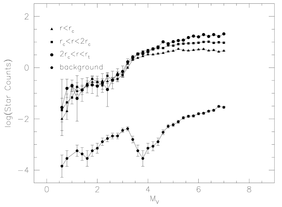
Figure 5: Stellar luminosity functions for the inner, $r\leq r_{c}$, intermediate, $r_{c}<r\leq 2r_{c}$, and outer, $2r_{c}<r\leq r_{t}$, annuli of M55. The color-selected field luminosity function (filled hexagons) is vertically shifted down for clarity.

Figure 5 shows clearly different behaviour of the LFs below the TO: they are similar for the stars above the TO, while the LFs become steeper and steeper from the inner to the outer part of the cluster: this is a clear sign of mass segregation. For the inner LF there is also a possible reversal in slope below $M_{V}=5.5$.

In order to verify that the difference between the three LFs is not due to systematic errors (wrong completeness correction, imperfect combination of data coming from two adjacent fields etc.), we have tested our combining procedure in several ways. In one of our tests we built LFs of two EMMI fields at the same distance from the center of the cluster: i.e., we compared the LF of the field 2 with that of the field 6. After having corrected for the ratio between the covered areas and subtracting the field star contribution, the two LFs were consistent in all the magnitude intervals down to the completeness level of the data (that is lower than the one adopted). Having for field 2 a magnitude limit of 22.2 (see Table 1) and field 6 a limit of 21.5, we also verified that for the latter our star counts are in correct proportion below the completeness level of 50%.

In a second test, we generated two LFs dividing the whole cluster in two octants (dividing along the $45^{\circ}$ line that runs from the center of the cluster till the field 19 cf. Figure 1). For each of the two slices we generated three LFs in the same radial range as in Figure 5. After comparing all of them we did not find any significant difference. Therefore the differences among the three LFs in Figure 5 must be real.

Figure 6: Mass functions for M55 for three radial ranges: inner, $r\leq r_{c}$, intermediate, $r_{c}<r\leq 2r_{c}$, and outer, $2r_{c}<r\leq r_{t}$. The effect of mass segregation is clearly visible. The slope $x$ corresponds to the index $x$ of the power law $\xi=\xi_{0}m^{-(1+x)}$ fitted to the data in the range $-0.23<\log(m/m_{\odot})<-0.1$.

Another source of error in the LF construction is represented by the LF of the field stars. As will be shown in Section 5, M55 has a halo of probably unbound cluster stars. The field star LF constructed from the star counts just outside the cluster can be affected by some contamination of the cluster halo. The consequence is that we might over-subtract stars when subtracting the field LF from the cluster LF, modifying in this way the slope of the mass function (the more affected magnitudes are the faintest ones). To test this possibility, we have extracted background LFs in two different anulii outside the cluster (in terms of $r_{t}$, $1.0<r\leq 1.3$ and $r>1.3$). Comparing the two background/foreground LFs we found that the number of stars probably belonging to the cluster but outside the tidal radius must be less than $\sim 25\%$ of the adopted field stars in the worst case (the faintest bins). The possible over-subtraction is not a problem for the inner and intermediate LFs, where the number of field stars (after rescaling for the covered area) is always less than $\sim 3\%$ of the stars counted in each magnitude bin. For the outer LF, the total contribution of the measured field stars is larger, but it is still less than $25\%$ of the cluster stars (the worst case applies to the faintest magnitude bin): this means that the possible M55 halo star over-subtraction in the field-corrected LF is always less than $6\%$ ($25\%\times 25\%$), negligible for our purposes.

4.1 Mass function of M55

In order to build a mass function for the stars of M55, we needed to adopt a distance modulus and an extinction coefficient. Shade et al. (1988) give $(m-M)_{V}=14.10$, E$(B-V)=0.14\pm 0.02$, while, more recently, Mandushev et al. (1996) give $(m-M)_{V}=13.90\pm 0.07$, E$(B-V)=0.14\pm 0.02$. In the absence of an independent measure made by us, we adopted the values published by Mandushev et al. (1996) because they are based on the application, with updated data, of the subdwarfs fitting method. Using the LFs of the previous Section we build the corresponding mass functions using the mass-luminosity relation tabulated by VandenBerg & Bell (1985) for an isochrone of $Z=3\times 10^{-4}$ and an age of 16 Gyr Alcaino et al. (1992). The MFs for the three radial intervals are presented in Figure 6. The MFs are vertically shifted in order to make their comparison more clear.

The MFs are significantly different: the slopes of the MFs increase moving outwards as expected from the effects of the mass segregation and from the LFs of Figure 5. Figure 6 clearly shows that the MF starting from the center out to the outer envelope of the cluster is flat: the index $x$ of the power law, $\xi=\xi_{0}m^{-(1+x)}$, best fitting the data are: $x=-2.1\pm 0.4$, $x=-0.8\pm 0.3$, and $x=0.7\pm 0.4$ going from the inner to the outer anulii; this means that the slope of the global MF (of all the stars in M55) should be extremely flat. Indeed, the slope of the global mass function obtained from the corresponding LF of all the stars of M55 is: $x=-1.0\pm 0.4$ This result agrees with the results of Irwin & Trimble (1984), while the results of Pryor et al. (1991) appear in contrast to what we have found here.

Our MF in the outer radial bin can be compared with the high-mass MF of Mandushev et al. (1996), obtained from a field located at $\simeq 6$ arcmin from the center of M55. As already reported in Section 2, Mandushev et al. (1996) obtained a deep MF for M55 (down to $M\simeq 0.1\mbox{$M_{\sun}$}$) which they describe with two power laws connected at $M\simeq 0.4\div 0.5\mbox{$M_{\sun}$}$. Their value of $x=0.5\pm 0.2$ for the high-mass end of the mass function ($0.5<M/\mbox{$M_{\sun}$}<0.8$) is in good agreement with our value of $x=0.7\pm 0.4$, obtained in the same mass range for the outer radial bin. The low-mass end of the MF by Mandushev et al. (1996) ($M/\mbox{$M_{\sun}$}<0.4$) has a slope of $x=1.6\pm 0.1$.

The level of mass segregation of M55 is comparable to that found in M71 by Richer & Fahlman (1989). M71 shares with M55 similar structural parameters as well as positional parameters inside the Galaxy. The detailed analysis of Richer & Fahlman (1989) of M71 showed that this cluster should also have a large population of very low mass stars ($\sim 0.1$$M_{\sun}$).

By fitting a multi-mass isotropic King model King (1966); Gunn & Griffin (1979) to the observed star density profile of M55, we compared the observed mass segregation effects with the one predicted by the models. Here we give a brief description of our assumptions in order to calculate the mass segregation correction from multi-mass King models. A more detailed description can be found in Pryor et al. (1991), from which we have taken the recipe. The main concern in the process of building a multi-mass model is in the adoption of a realistic global MF for the cluster. For M55 we adopted a global MF divided in three parts:

• a power-law for the low-mass end, $0.1<M/\mbox{$M_{\sun}$}\leq 0.5$, with a fixed slope of $x=1.6$ (as found by Mandushev et al. 1996);

• a power-law for the high-mass end, $0.5<M/\mbox{$M_{\sun}$}\leq m_{TO}$, with a variable slope $x$;

• and a power-law for the mass bins of the dark-remnants where to put all the evolved stars with mass above the TO mass, $m_{TO}<M/\mbox{$M_{\sun}$}\leq 8.0$: essentially white dwarfs. Here we adopted a fixed slope of 1.35, The mass of the WDs were set according to the initial-final mass relation of Weideman (1990).

Figure 7: Isotropic King model MF slope correction for M55. The full dots are the slopes of the MFs obtained in this paper, the open circle is the measure of the high-end MF of Manddushev et al., 1996.

Figure 8: Trivariate relation from Zoccali et al.(1997), between the distance from the Galactic center ($R_{GC}$), the height above the Galactic plane ($Z_{GP}$), the metallicity of the cluster ([Fe/H]), and the slope of the global stellar mass function ($X_{0}$) of a globular cluster. The filled square marks the position of M55.

To build the mass segregation curves we varied the MF slope $x$ (the only variable parameter of the models) of the high-mass end stars in the range $-1.0\div 1.35$, finding for each slope the model best fitting the radial density profile of the cluster. Then we calculated the radial variation of $x$ for the best-fit models in the same mass range of the observed stars: $0.5<M/M_{\odot}<m_{TO}$. The radial variations of $x$ are compared with the observed MFs in Figure 7. The mass function slopes are shown at the right end of each curve. This plot is similar to those presented in Pryor et al. (1986), and allows one to obtain the value of the global mass function of the cluster. The three observed points follow fairly well the theoretical curves. Also the high-mass MF slope value of Mandushev et al. (1996) (open circle in Figure 7) is in good agreement with the models and our MFs. From these curves, we have that the slope of the high-mass end of the global MF of M55 is $x\simeq-1.0$, which is in quite good agreement with the global value of the MF found from the global LF of M55 (cf. previous section). In Figure 9 we show the model which best fits the observed radial density profile for a global mass function with a slope $x=-1.0$.

The relatively flat MF of M55 could be the result of the selective loss of main sequence stars, especially from the outer envelope of the cluster, caused by the strong tidal shocks suffered by M55 during its many passages through the Galactic disk and near the Galactic bulge (Piotto, 1993, for a general discussion of the problem). A flat MF for M55 agrees well with the results of Capaccioli et al. (1993) who have found that the clusters with a small $R_{GC}$ and/or $Z_{GC}$ show a MF significantly flatter than the cluster in the outer Galactic halo or farther from the Galactic plane. Indeed, M55 is near to the Galactic bulge, $R_{GC}=4.7$ kpc ($R_{\odot}=8.0$ kpc), and to the Galactic disk $Z_{GC}=-2.0$ kpc. Figure 8 shows that taking into account observing errors, M55 fairly fits into the relation given by Zoccali et al. (1997), which is a refined version of the one found by Djorgovski et al. (1993). A different conclusion has been reached by Mandushev et al. (1996) using their uncorrected (for mass segregation) value for the MF of M55. As noted by the referee, M55 lies further from the average relation defined by the other clusters: of those with a similar abscissa ($0.0\pm 0.2$), M55 is the one with the lowest value of $x$. It is not possible to identify the main source of this apparent enhanced mass-loss of M55 compared to the other clusters; a possible cause can be a orbit of the cluster that deeply penetrate into the bulge of the Galaxy. This cannot be confirmed until is performed a reliable measure of the proper motion of M55.

Figure 9: Radial density profile of M55. Small crosses represent the raw stellar counts; filled dots are our star counts after subtracting the background counts contribution; open dots shows the M55 profile published by Pryor et al.(1991); the continuous line is the single mass King model fitted to our star counts ($c=0.83,\,r_{c}=143^{\prime\prime}$).

5 Radial density profile from star counts.

The CMD allows a unique way to obtain a reliable measure of the radial density profiles of GCs. In fact, the CMD allows us to sort out the stars belonging to the cluster, limiting the problems generated by the presence of the field stars. This also permits to extract radial profiles for distinct stellar masses.

We have first created a profile as in King et al. (1968), in order to compare our results with the existing data in the literature. The comparison has been done with the radial density profile of M55 published by Pryor et al. (1991) which includes the visual star counts of King et al.. We could not compare our data with Irwin & Trimble (1984) because they have not published their observations in tabular form.

Figure 10: Radial density profile of M55 for different magnitude intervals. All the profiles has been smoothed in the external parts. In the graph the positions of $r_{c}$, 2$r_{c}$ and $r_{t}$ are shown. The profiles have been normalized in the radial range $2.6<\log(r)<2.9$.

5.1 Density profile for stars above the TO

Figure 9 shows the radial density profile for the TO plus SGB stars extracted from the CMD of M55 (from 1 magnitude below the TO to the brightest limit of our photometry). We have selected the stars within $2.5\sigma$ from the fiducial line of the CMD plus the contribution coming from the BS and HB stars; star counts has been limited at the magnitude $V\leq 18.5$. This relatively bright limit corresponds approximately to the limit of the visual star counts by King et al. (1968) on the plate ED-2134 (in order to make the comparison easier we used the same radial bins of King). Our counts have been transformed to surface brightness and adjusted in zero point to fit the Pryor et al. (1991) profile of M55.

The agreement with the data presented by Pryor is good everywhere but in the outer parts where our CCD star counts are clearly above those of King et al. (1968). This difference is probably due to our better estimate of the background star contamination. In the plot we have shown also the raw star counts (crosses) prior to the background star subtraction: it can be clearly seen that our star counts go well beyond the tidal radius, $r_{t}=977^{\prime\prime}$, published by Trager et al. (1995). This allow us to estimate in a better way than in the past the stellar background contribution. The background star counts show a small radial gradient: we will discuss this point in greater detail in the next Section. Here, the minimum value has been taken as an estimate of the background level.

We point out that the differences present in the central zones of the cluster could be in part due to some residual incompleteness of our star counts, to the absence in the starcounts of the brightest saturated stars, and to the difficulties in finding the center of the cluster. We searched for the center using a variant of the mirror autocorrelation technique developed by Djorgovski (1988). In the case of M55 we encountered some problems due to a surface density which is almost constant inside a radius of $\simeq 100\arcsec$.

In order to evaluate the structural parameters of M55, we have fitted the profile Figure 9 with a multi-mass isotropic King (1966) model as described in the previous Section. In the following table we show the parameters of the best fitting model and we compare them with the results of Trager et al. (1995), Pryor et al. (1991), and Irwin & Trimble (1984):

Author	$c$	$r_{c}$	$r_{t}$
This paper	0.83	$143^{\prime\prime}$	$970^{\prime\prime}$
Trager et al.	0.76	$170^{\prime\prime}$	$977^{\prime\prime}$
Pryor et al.	0.80	$140^{\prime\prime}$	$876^{\prime\prime}$
Irwin and Trimble	$\sim 1.0$	$\sim 120^{\prime\prime}$	$\sim 1200^{\prime\prime}$

The concentration parameter of M55 is one of the smallest known for a globular cluster. Such a small concentration implies strong dynamical evolution and indicates that the cluster is probably in a state of high disgregation Aguilar et al. (1988); Gnedin & Ostriker (1997).

Our value of the tidal radius is well in agreement with that of Trager et al. (1995) who used a similar method to fit the data. Pryor et al. (1991) give a value of $r_{t}$ 10% smaller than ours. We note that Pryor and Trager used the same observational data set. The difference with Irwin & Trimble (1984) is probably due to the fact that the authors have not fitted their data directly but made only a comparison with a plot of King models.

Figure 11: Radial density profile of M55 for different magnitude intervals. An arrow marks the position of $r_{t}$. The profiles are normalized in the radial range $1.0r_{t}<r<2.0r_{t}$ to better compare the extra-tidal profiles. We show also the power law interpolation of the profiles.

5.2 The density profile for different stellar masses.

Having verified the compatibility of our density profile with previously published ones, we have extracted surface density profiles for different magnitude ranges corresponding to different stellar masses. The adopted magnitude intervals have been chosen to have a significant number of stars in each bin. We used logarithmic radial binning that allows a better sampling of the stars in the outer part of the cluster. In order to lower the noise in the outer part of the profile, we have smoothed the profiles with a median static filter of fixed width of 3 points. We verified that the filtering procedure did not introduce spurious radial gradients in the density profiles. The mean masses in each magnitude bin adopted for the profiles, as obtained from the isochrone by VandenBerg & Bell (1985) (cf. also Section 4.1), are:

$V$	$<m>$
$<18$	0.79
$18-19$	0.77
$19-20$	0.71
$20-20.9$	0.63

The relative profiles, without subtraction of the background stars, are shown in Figure 10 and 11. The arrows in both figures indicate $r_{c}$, $2\leavevmode\nobreak\ r_{c}$ and $r_{t}$.

The profiles plotted in Figure 10 are clearly different from each other: this is as expected from the mass segregation effects. To better compare the profiles, in Figure 10 they have been normalized in the radial interval $2.6<\log(r/arcsec)<2.9$ (where the profiles have a similar gradient) to the profile of the TO stars. This operation is possible because in this radial range the effects of mass segregation are small (cf. Figure 7); they are more evident within one core radius. The density profiles are consistent with the mass segregation effects that we have already seen in the mass function of the cluster.

The more interesting aspect of the profiles in Figure 10 is the clear presence of a stellar radial gradient in the star counts of the background field stars. In Figure 11, we show the radial profiles of the extra cluster stars after normalization of the profiles outside $\log(r/arcsec)=3.0$. The 4 profiles are not exactly coincident outside $r_{t}$. Let us discuss various possible explanations for this observation:

• Errors in the completeness correction or errors in the star counts. We repeated the extensive tests on the data made to assess the validity of the mass segregation seen in the LFs. We checked that the variation in the completeness limit of the various EMMI fields does not introduce spurious trends. In a different test, we divided the cluster in two slices along a line at $45^{\circ}$ from the center of the cluster up to the field 19 (cf. Figure 1), and built the radial profiles for each of the 4 magnitude bins: in all cases there were no significant differences. The radial profile of the stars in the magnitude range $18\div 19$ ($M_{V}=4.1\div 5.1$ in Figure 5) has the lowest contamination of background stars, as shown by its LF in Figure 5.

• A non-uniform distribution of the field stars around M55. It is possible that the field stars around M55 are distributed in a non-uniform way. In the work by Grillmair et al. (1995) it clearly appears that the field stars of some GCs present a non-uniform distribution around the clusters. The gradients are significant and the authors used bidimensional interpolation to the surface density of the field stars to subtract their contribution to the star counts of the clusters. In the present case, field star gradients could be a real possibility, but we cannot test it because we do not have $360^{\circ}$ coverage of the cluster: our coverage of M55 is only a little more than a quadrant. The Galactic position of M55 ($l\simeq-23^{\circ}$, $b\simeq 9^{\circ}$) can give some possibility to this option. At this angular distance from the Galactic center the bulge and halo stars probably have a detectable radial gradient. However it remains difficult to explain the existence of the gradient also for the stars in the magnitude range $18\div 19$: for them (cf. section 4), as stated before, we have the lowest contamination from the field stars.

  We have created a surface density map of the starcounts of M55. The map was constructed using all the stars of the $2.5\sigma$-selected sample of our photometry (excluding fields 25 and 35), counting stars in square areas of approximately $9^{\prime\prime}\times 9^{\prime\prime}$ and then smoothing the resulting map with a gaussian filter. The starcounts are not corrected for crowding but we stopped at $V=20.5$. The map is presented in Figure 12. The map has the same orientation as Figure 1. We have also overplotted contour levels to help in reading the map. Figure 12 clearly shows that well outside the tidal radius of M55 (located approximately at the center of the map) there is a visible gradient in the star counts.

• A gradient generated by the presence of the dwarf spheroidal in Sagittarius Ibata et al. (1995). Between the Galaxy center and M55 there is the dwarf spheroidal galaxy called Sagittarius Ibata et al. (1995). Sagittarius is interacting strongly with the Galaxy and probably is in the last phases of a tidal destruction by the Galactic bulge. The distance between the supposed tidal limit of this galaxy (using the contour map of Ibata et al.1995) and M55 is $\sim 5^{\circ}$. In the recent work by Mandushev et al. (1996) the giant sequence of the Sagittarius appears clearly overlapped with the sequence of M55. This happens only in the magnitude range $V\simeq 20.0\div 21.0$ where our star counts end. Fahlman et al. (1996) showed that the SGB sequence of the Sagittarius crosses the main sequence of M55 at $V\simeq 20.5\div 20.7$, and at a corresponding color of $(V-I)\simeq 1.1\div 1.2$. Similar results were found by Mateo et al.. (1996). This is due to the different distances of these two systems from us: $\sim 4.5$ kpc for M55 and $\sim 24$ kpc for Sagittarius. This implies that out star counts can be influenced by the stars of the dwarf spheroidal only in our last magnitude bin, $20\div 20.9$. Our selection of stars along the CMD of M55 limits the Sagittarius stars to those effectively crossing the main sequence. In conclusion, if effectively the Sagittarius stars are present as background stars we should see them only in one of the 4 profiles, but the coincidence of the 4 profiles excludes this ipothesis.

• A halo of stars escaping from the clusters. This possibility is more suggestive. The stellar gradient could be a possible extra-tidal extension of the cluster, similar to what Grillmair et al. (1995) found in their sample of 12 clusters. The tidal extension could be caused by the tidal-shocks to which the cluster has been exposed during its perigalactic passages, through the Galactic disk. Another possibility is the creation of the stellar halo by stellar dynamical evaporation from the inner part of the cluster. Such mechanisms work independently of stellar mass Aguilar et al. (1988) and so the stellar halo should have a similar gradient for all the stellar masses as in the present case. Such halos are very similar to the theoretical results obtained by Oh & Lin (1992) and Grillmair et al. (1995), who have obtained tidal tails for globular clusters N-bodies simulations.

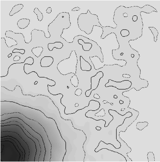
Figure 12: Surface density map of M55 with contour levels.

We believe that the probable explanation for the phenomenon shown in Figures 10 and 11 is in the presence of an extra-tidal stellar halo or tidal tail. Doubt resides in the unknown gradient of the background field stars. To resolve this we need to map the whole cluster and a large area surrounding the cluster. This would also allow us to find the exact level of field stars. Our star counts stop at 33′($\simeq 2\times r_{t}$), from the center of M55 while the tidal tails of Grillmair et al. (1995) stop at $\simeq 2.5\div 4\,r_{t}$. Consequently, we cannot correctly subtract the contribution of the field stars from our star counts. We can give only an estimate of the exponent of the power law, $f\propto r^{-\alpha}$, fitting the profiles at $r>1.2\,r_{t}$. Without subtracting any background counts $\alpha\sim 0.7\pm 0.3$, while subtracting different levels of background stars the slope varies in the interval $0.7<\alpha<1.7$: the highest value comes out after subtracting the outermost value of the density profiles. When it will be available a better estimate of the background/foreground level of the sky it will be possible to assign a value to the slope of the gradient of stars: actually our range, $\alpha=0.7\div 1.7$, is in accordance with those found theoretically by Oh & Lin (1992) and observationally by Grillmair et al. (1995).

Table 1: For each field of M55 we list the total number of detected stars in both the $V$ and $I$ frame, the mean airmass of the field, the right ascension and the declination of the field center, the FWHM of the $V$ and $I$ point spread functions of the images, and the $V$ limit magnitude of the observed fields. For each $V$ image the exposure time was of 40 seconds, while for the $I$ image it was of 30 seconds.

Field	Stars	Airmass	RA	DEC	FWHM		V(50%)
			[deg]		$V$	$I$
01	13442	1.010	294.926	$-30.948$	0.9	0.9	21.0/22.1
02	3176	1.007	295.062	$-30.948$	0.9	0.9	22.2
03	872	1.004	295.198	$-30.948$	1.1	1.1	22.1
04	495	1.005	295.333	$-30.947$	1.3	1.1	21.2
06	2273	1.016	294.926	$-30.831$	1.3	1.2	21.5
07	800	1.013	295.061	$-30.831$	1.5	1.5	21.2
08	543	1.009	295.197	$-30.831$	1.4	1.4	21.2
09	482	1.007	295.333	$-30.831$	1.6	1.6	21.0
11	635	1.022	294.926	$-30.714$	1.4	1.4	21.3
12	560	1.028	295.061	$-30.714$	1.4	1.4	21.2
13	531	1.034	295.197	$-30.714$	1.4	1.5	21.0
14	506	1.041	295.333	$-30.714$	1.3	1.5	21.0
16	491	1.227	294.983	$-30.598$	1.3	1.4	20.9
17	503	1.150	295.061	$-30.598$	1.6	1.3	20.9
18	537	1.055	295.197	$-30.598$	1.5	1.6	21.1
19	556	1.048	295.332	$-30.598$	1.3	1.5	21.2
25	666	1.001	295.197	$-31.063$	1.2	1.3	21.6
35	757	1.001	295.333	$-31.063$	1.2	1.1	21.9

Appendix A Image reduction and analysis

The images were reduced using the standard algorithms of bias subtraction, flat fielding and trimming of the overscan, without encountering particular problems. The stellar photometry was done using DAOPHOT II and ALLSTAR Stetson (1987). The second version of DAOPHOT was particularly useful for the image analysis since we were forced to use a variable point spread function (PSF) through the images. In fact, the stellar images of the EMMI Red Arm together with the F/2.5 field camera presented coma aberration at the edges of the field: the resulting PSF was radially elongated. To better interpolate the PSF we also used an analytic function with 5 free parameters (i.e. the Penny function of DAOPHOT II).

In order to obtain a single CMD for all the stars found in the 18 fields we first obtained the CMD of each field matching the $V$ and I photometry. Then, we combined all the CMDs using the relative zero points determined from the overlapping regions of adjacent fields. All the CMDs were connected to the main CMD, one at a time, following a sequence aimed at maximizing the number of common stars usable for the zero point calculation. The central field CMD was used as the starting point of the combination. For the outer fields we used a minimum of 20 common stars while for the inner fields we had at least 300 stars. The mean error of the zero points was $\simeq 0.05$ magnitudes, compatible with the errors calculated from the crowding experiments. Since the night was not photometric, we could not directly calibrate our data. We were only able to set an absolute zero point using the unpublished calibrated photometry of the center of M55 by Piotto (see next Section).

In order to perform the photometry of the central field of the cluster, we divided it into 4 subimages of $\simeq 600\times 600$ pixels, to minimize the effect of the strong stellar gradients present in this image. We allowed a good overlap to be able to perform the successive combination of the photometry of the stars. In this way we also avoided two problems: we had better control of the PSF calculation and we reduced the number of stars per image to be analyzed. Thanks to the low central concentration of the cluster and the fairly good seeing of the images (even if the crowding was not completely absent), we were able to obtain complete photometry down to $V\simeq 21$.

Figure 13: top: Differences between our instrumental $V$ magnitude ($V_{raw}$) and the calibrated magnitude by Alcaino et al.(1992) ($V_{Alcaino}$). Bottom: Differences between our instrumental color, $(V-I)_{raw}$, and the calibrated color by Alcaino (1992), $(V-I)_{Alcaino}$.

Figure 14: Differences between our instrumental $V$ magnitude ($V_{raw}$) and the calibrated magnitude of Piotto (1994) ($V_{Piotto}$).

Appendix B Calibration of the photometry

In principle, the analysis of the radial density profile does not require calibrated photometry. But this operation is necessary if we want to analyze the stellar population of the cluster, together with its stellar luminosity and mass functions. Since we could not use standards taken during the same night, we have performed a relative calibration using existing photometry of M55. For the $V$ magnitude we linked our data to Piotto’s (1994) un published photometry of the central field of M55 from images taken with the 2.2 m ESO telescope. For the (V-I) we calibrated our data against Alcaino et al. (1992) photometry. They published a CCD BVRI photometry for two different non-overlapping fields outside the center of M55, named FA and FB, with dimensions of $3\aas@@fstack{\prime}1\times 1\aas@@fstack{\prime}9$, contained in our central field. Figure 14 shows our $V$ zero point calculated against Piotto’s (1994) while Figure 13 shows the $V$ zero point of the two fields FA and FB of Alcaino et al. (1992). The mean zero point for the two fields of Alcaino et al. gives $\Delta V_{Alcaino}=6.11\pm 0.04$ which compare well with $\Delta V_{Piotto}=6.12\pm 0.03$. The two are in good agreement taking into account the errors. There are no magnitude gradients. The LFs are coming from the photometry in the V-band.

Before the publication of the I-band photometry by Mandushev et al. (1996), the one by Alcaino et al. (1992) was the only photometry in the literature. Unfortunately, the M55 data set of Mandushev et al. (1996) does not overlap with any of our fields: it is centered just few arcmin south of our field 2. In Figure 13, we show the difference between our data and those of Alcaino et al. (1992). In this case, the two zero points calculated for Alcaino’s fields differ by a significant amount. We do not know the origin of this discrepancy, which we believe is internal to the data of Alcaino et al. (1992). They could not resolve this due to the fact that fields FA and FB do not have stars in common. We believe that the problem is not in our data since both Alcaino’s fields are contained in the same subimage of the central field. Lacking other independent (V-I) calibrations, we are forced to adopt as our color zero point the mean of the two values of FA and FB: $\Delta(V-I)=0.45\pm 0.05$.

Appendix C Crowding experiments.

For each field, we performed a series of Monte Carlo simulations in order to establish the magnitude limit and the degree of completeness of the CMD. The magnitude limit has been defined as the level at which the completeness function reach a value of $0.5$, V(50%). This value is reported in Table 1 for each field.

The procedure followed to generate the artificial stars for the crowding experiments is the standard one Piotto et al. (1990b). The completeness function used to correct our data is the combination of the results of the experiments in both the $V$ and $I$ images for each field. In the outer fields the stars were added at random positions in a magnitude range starting from $V=19$ (just 0.5 mag below the main sequence TO). In the $I$ band experiments, we used the same star positions of the $V$ experiments, with the $I$ magnitudes set according to the corresponding main sequence color. For each outer field, we performed 10 experiments with 100 stars. For the inner fields (fields number 2, 3 and 6) the experiments were 10 with 100 stars in an interval of only 1 magnitude for 5 different magnitudes (a total of 50 experiments). Moreover, in these fields the stars were added taking into account the radial density profile of the cluster. For the 4 subimages of the central field, we performed independent crowding experiments. For each subimage, we ran 10 experiments in 0.5 mag. steps in the range $19\div 23$, with the stars radially distributed as the density profile of the cluster. In this way, we were able to better evaluate the level of the local completeness of the photometry.

The completeness function has been calculated for each field taking into account the results of the two different experiments in $V$ and I. As an example in Figure 15 we show the completeness functions for field number 3 (top) and 19 (bottom). The results of the experiments were fitted using the error function:

$$g(x;y_{0},\sigma)=1-\int_{-\infty}^{x}e^{\frac{(y-y_{0})^{2}}{\sigma^{2}}}{\rm d}y.$$ (1)

$y_{0}$ is the magnitude at which the completeness level is 50%, V(50%); $\sigma$ gives the rapidity of the decrease of the incompleteness function and is connected with the read out noise and the crowding of the image. For the star counts correction we used the interpolation with the previous equation instead of using directly the noisy results of the experiments (these were too few to lower the small number statistical noise of the results). In this way we avoid the adding of noise to the star counts. In every case we verified that the fitting function is an acceptable interpolation that gives very low residuals compared to the error distribution function.

Figure 15: Top: Completeness function for the field number 3. Bottom: Completeness function for the field number 19. Both functions have been obtained combining the crowding experiments on in $V$ and I.