This document can be retreived as a postscript file via the web and internet on the CERN preprint server: http://preprints.cern.ch/ or on the following servers http://infodan.in2p3.fr/antares/docs.html http://marcpl1.in2p3.fr/antares/docs.html

Preamble

This document is mainly intended to describe the Astroparticle aspect of ANTARES. The Sea Science part of the project is described in [1].

Introduction

We propose to observe High Energy Cosmic Neutrinos using a deep sea Cherenkov detector. In what follows, we will elaborate on the potential interest of such a study for Astrophysicists and Particle Physicists. For Oceanologists participating in the collaboration, the main goal is a long term measurement of environmental parameters in the deep sea.

The physics detector principle is based on the detection of Cherenkov light emission in either ice or water of upward going muons induced by neutrino interactions in the medium surrounding the detector.

AMANDA [2] is a running experiment installed at the South Pole, for which it has been demonstrated that deployment and logistics problems can be solved. It still remains to be demonstrated that the quality of the ice allows an accurate measurement of the neutrino direction.

BAIKAL [3] is another running experiment installed in lake Baikal, for which the feasibility as well as the capability to reconstruct up going and down going muons have been shown. The relatively poor transparency of the water and the shallow depth of the lake may be a limitation for further extensions. Moreover, optical properties of deep sea water have been measured to be better than those of lake water.

DUMAND [4] was a pioneer for studies about deep ocean water detectors. The funding of this project has been cancelled in 1996 by DOE [5].

NESTOR [6] is a project planned to be installed in a deep sea site offshore from Pylos, Greece. Preliminary work started in 1989. The first step will be the installation of a few optical modules connected via an electro-optical cable to the shore and later of a complete tower.

In terms of depth, servicing and optical properties a deep-sea detector is promising. We propose to explore the possibility of a km-scale detector to be installed in a deep site in the Mediterranean sea, for which a broad collaboration will be needed. Furthermore, a variety of technical problems have to be solved. Some of them are standard for particle physicists (choice of photo-multipliers, monitoring, trigger, electronics and data acquisition, analysis tools…), although the constraints coming from the deep sea environment and the lack of accessibility have to be fully taken into account. Others are more specific of sea science engineering, namely detector deployment in deep water, data transmission through optical cables, corrosion, bio-fouling of optical modules, positioning. We have found technical support from collaborators and partners which have experience in this field (COM, CSTN, CTME, IFREMER, France Télécom Câbles, INSU-CNRS…).

We will test the sea engineering part of a detector including test deployments close to the Toulon coast (France) where technical support is available and where several sites at depths down to 2500 m are easily accessible. During the same time, issues connected to the accomplishment of a large scale detector and the selection of an optimum site will be addressed.

We propose to build and install a demonstrator (a fully equipped 3-dimensional test array) the design of which can be extended to a km³ scale detector. We plan to reach this goal within the next 2 years.

1 Scientific motivation

The ANTARES project addresses several physics topics which have in common the need for a long exposure of a large detector shielded from charged cosmic rays.

In what follows, we will mainly describe the Astroparticle aspects of the project. Only a few examples of possible Sea Science studies will be mentioned.

1.1 Scientific motivation in Particle Physics and Astrophysics

1.1.1 Introduction

In Particle Physics, the unification of the four known forces has been and still is a major goal in the quest for our understanding of the Universe. In the framework which is generally accepted, all the forces are unified at very high energy. In order to have access to much higher energies than available at LHC in the near future, Big Bang relics or active cosmic objects can be used as providers of Ultra High Energy particles (in excess of 10²⁰ eV, as already detected on Earth [7]). How Nature is able to accelerate particles to energies far beyond human possibilities is still an unanswered question. Taking advantage of the available cosmic particles, the study of Ultra High Energies could help us, on one hand, to test various models of acceleration mechanisms, and on the other hand, to constrain the different candidate theories which aim at extending the Standard Model up to the Planck scale.

The supersymmetric extensions of the Standard Model [8], predict the existence of at least four neutralinos, linear combinations of the two superpartners of the neutral SU(2) gauge bosons (gauginos) and the two superpartners of the neutral Higgs particles (higgsinos). In most of the models, the lightest neutralino is the Lightest Supersymmetric Particle and thus is a candidate for dark matter. So, even if superparticles were discovered at accelerators, it would still be of major interest to constrain both supersymmetric and cosmological models by observing neutrinos produced in the annihilation of neutralinos remnants of the Big Bang.

The atmospheric neutrino flux can also be studied for neutrino oscillations.

A High Energy Neutrino detector may open a new observation window on the Universe, complementary to the photonic observations already in use, and help with the elucidation of the origin of the Ultra High Energy Cosmic Rays already observed.

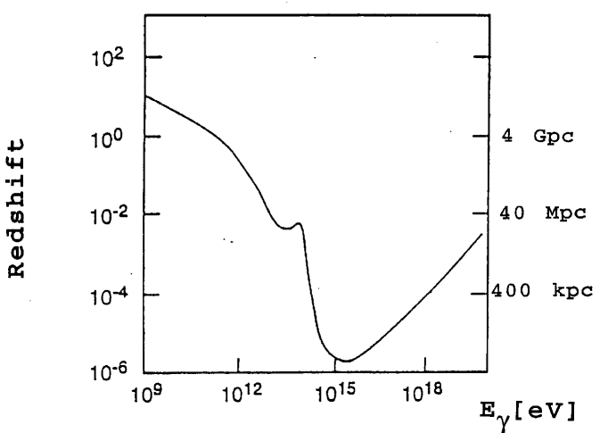
Figure 1: Attenuation length of cosmic photons as a function of their energy $E_{\gamma}$. The attenuation is due the interactions of these photons on the IR and microwave cosmic backgrounds.

The use of neutrinos to observe the Universe has some intrinsic advantages. Charged particles are sensitive to magnetic fields, at the source, during their transport and in the Galaxy; so, except for those with ultimate energies, they do not point to their emission source. In contrast, neutrinos and photons are insensitive to those magnetic fields. However, high energy photons are absorbed by a few hundred g.cm^-2, when the interaction length of a 1 TeV neutrino is about 250 10⁹ g.cm^-2. Furthermore interactions of Very High Energy photons with the infrared radiation and Cosmic Microwave Background (2.7 K) limit their path length to distances smaller than 100 Mpc (see fig. 1).

Because they could originate from a common source, the combined study of both the energy spectra of $\gamma$-rays and neutrinos emitted by cosmic sources is necessary in order to tackle the question of the origin of the highest energy cosmic rays and the nature of the mechanisms capable of producing them.

A variety of $\gamma$-ray detectors are already operating. These detectors allow to explore the GeV region (satellites) and above 200 GeV (large arrays and ground based Cherenkov imaging telescopes) [9, 10, 11]. These detectors have already shown evidence of point-like celestial $\gamma$-ray sources.

As for cosmic neutrinos, a few examples of their detection exist at low energies. Let us mention the detection of the signals of solar neutrinos [12], below $\approx$ 10 MeV, and of neutrinos from the supernova SN1987A [13], at a few tens of MeV. It is, thus, of major interest to explore the possibility to detect signals at higher energies. Several attempts have been made with underground detectors, part of them devoted to proton decay detection. Due to the modest dimensions of such detectors ($\leq$ 1000 m²), only upper limits on the neutrino luminosities of several celestial bodies were obtained [14, 15]. The expected fluxes of high energy neutrinos actually require a km-scale detector (see section 1.1.4).

1.1.2 High Energy Neutrino production

• Neutrinos of cosmic acceleration origin:
  Point-like cosmic photon sources have been observed in the TeV range by the ground based observatories [11]. Two mechanisms are possible for the production of these photons [7]. The electromagnetic one is based on synchrotron radiation emitted by accelerated plasma followed by inverse Compton scattering on electrons. The hadronic one is based on the decay of $\pi^{0}$’s produced in hadronic interactions of accelerated nucleons with a cosmic target (matter or photon field).

  The first mechanism does not produce any neutrinos. The second one, in contrast, gives rise to neutrino production coming from the decay of charged pions produced together with the neutral ones.

  $$p/A+p/\gamma\longrightarrow\begin{array}[t]{l}\pi^{0}\\ \downarrow\\ \gamma+\gamma\end{array}+\begin{array}[t]{l}\pi^{+}\\ \downarrow\\ \mu^{+}+\nu_{\mu}\\ \downarrow\\ e^{+}+\nu_{e}+\overline{\nu}_{\mu}\end{array}+\begin{array}[t]{l}\pi^{-}\\ \downarrow\\ \mu^{-}+\overline{\nu}_{\mu}\\ \downarrow\\ e^{-}+\overline{\nu}_{e}+\nu_{\mu}\end{array}+...$$

  Depending upon the precise characteristics of the cosmic beam dump and the ratio of charged to neutral pions, the $\nu/\gamma$ ratio, at a distance from the source, can take any value between the $\nu/\gamma$ ratio at production (leaky source) and infinity (shrouded source) [7].

  As the highest energy cosmic rays detected on Earth are very likely protons, it is unavoidable that cosmic neutrinos are created from their interactions with matter and the Cosmic Radiation Background.

  Possible galactic sources are:

  • X-ray binary systems. They are made of a compact star, such as a neutron star or a black hole, which accretes the matter of its non compact companion. Strong magnetic fields combined to plasma flows lead to a stochastic acceleration of particles by resonant interaction with plasma waves in the magnetosphere of the compact star. The interaction of the accelerated particles with the accreted matter or the companion itself produces mesons which eventually decay into neutrinos.

  • Young supernova remnants. Protons inside supernova shells can be accelerated in the magnetosphere of the pulsar, by a first order Fermi mechanism in case of turbulence in the shell or at the front of the shock wave produced by the magneto-hydrodynamic wind in the shell [16]. The interaction of these protons with the matter of the shell gives rise to neutrino emission. The active neutrino phase lasts from 1 to 10 years after the supernova explosion. Recent observations [10] above 100 MeV by the EGRET detector have found $\gamma-$ray signals associated with at least 2 supernova remnants (IC 443 and $\gamma$ Cygni).

  As for extra-galactic sources:

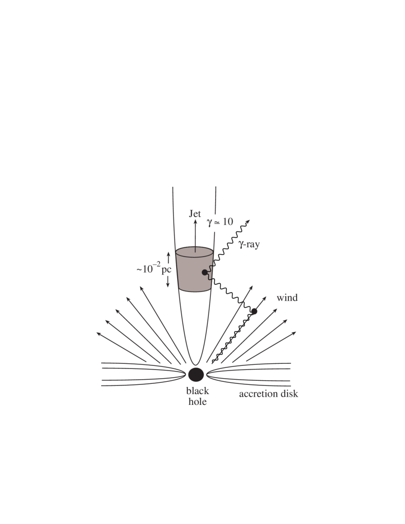
Figure 2: A possible model for the production of high energy photons and neutrinos in an AGN [18].

  • Active Galactic Nuclei (AGNs) are good candidates. These galaxies are the brightest objects in the Universe. Their powerful and compact central engine is thought to be made of a supermassive black hole (10⁴-10¹⁰ solar masses). The energy powering the engine comes from the accretion of the matter surrounding the black hole at a rate of a few solar masses per year, leading to total luminosities in the range 10⁴²-10⁴⁸ erg/s [17]. Different acceleration sites in the AGNs are envisioned (see fig. 2 and [18]), namely:

    • close to the central engine,

    • along the radio jets,

    • in hot spots terminating the jets in the radio lobes,

    leading to possible neutrino generation by interaction of accelerated protons with surrounding matter in the central core (pp) or with dense photon fields in jets (p$\gamma$). Emission of $\gamma$-rays up to $\approx$ 10 GeV from Active Galactic Nuclei have been well established by EGRET [9]; two of them (Mrk 421 and Mrk 501) have been also observed as emitters of high energy gamma rays (above 1 TeV) by ground based observatories [11].

  • We may include in the potential extra-galactic sources Gamma Ray Bursts although it cannot yet be excluded they might be located in the extended Galactic halo. GRB’s have been observed for many years and recent detectors observed bursts at a rate of one per day. Their location was first thought to be galactic, now extra-galactic (cosmological) models are strongly favored [19]. GRB’s are expected to emit a big part of their energy in neutrinos [20, 21]. Recently, emission of neutrinos of very high energies from GRB fireballs was predicted [22]. The observation of gamma, X, optical and radio signals from GRB 970228 and GRB 970508 [23] (estimated to be at z $\geq 0.85$ ) is in agreement with this model.

  By their very existence, galactic and extra-galactic cosmic rays guarantee the production of high energy cosmic neutrinos. Indeed, the primary cosmic rays can interact with:

  • the production medium,

  • the Cosmic Microwave Background (2.7 K) [24],

  • interstellar gas in our galaxy [17],

  • the Earth atmosphere [25],

  to produce mesons which eventually decay into neutrinos.

• Neutrinos of non-acceleration origin:
  Topological defects (cosmic strings, monopoles) [26] and non baryonic dark matter [17] bring into play very heavy entities which by quantum evaporation, collapse or annihilation eventually give rise to an emission of high energy neutrinos.

  • Monopoles and cosmic strings are topological defects likely to have been formed in the symmetry breaking phase transitions that occured in the early Universe. Inside these defects, the vacuum expectation value is 0 while everywhere else it is of the order of the symmetry breaking scale ($\sim 10^{16}$ GeV). These defects are stable but can be destroyed by collapse or annihilation [27], releasing the energy trapped in them in the form of massive quanta $X$ which eventually decay into hadrons, leptons, photons and neutrinos with energies up to $m_{X}\sim 10^{16}$ GeV. The rate of release of $X$ particles is given by:

    $$\frac{dN_{X}}{dt}=\kappa m^{p}_{X}t^{-4+p}$$

    where $t$ is the Hubble time. $\kappa$ and $p$ are dimensionless constants the value of which depends on the characteristics of the topological defects:

    • $p=0$ for saturated superconducting cosmic string loops,

    • $p=1$ for collapsing cosmic string loops and annihilating monopole-antimonopole bound states.

  • Neutralinos, remnants from the Big Bang, move in the halo of the Galaxy with velocity of a few hundred km/s. They can encounter celestial bodies, lose energy by elastic scattering on the nuclei these bodies are made of, and stay trapped in them. This results in a high concentration of neutralinos in the Sun and the Earth which enhances their annihilation rate per unit volume giving rise, amongst others, to a neutrino emission [8].

1.1.3 Detection of High Energy Cosmic Neutrinos

• Detection principle:
  All potential sources produce $\nu_{e}$’s as well as $\nu_{\mu}$’s. One could detect $\nu_{e}$ interactions by observing electromagnetic and hadronic showers of contained events. However, at this stage, we will only concentrate on $\nu_{\mu}$ detection.

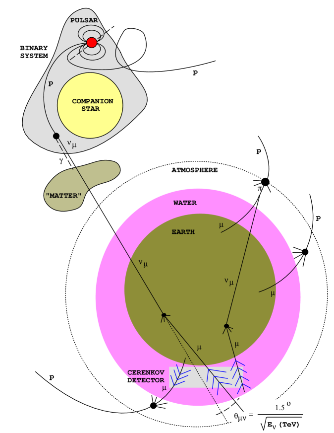
Figure 3: Neutrino detection principle

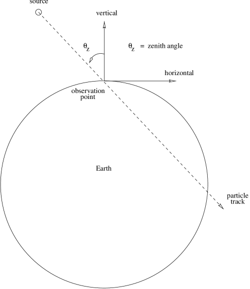
Figure 4: Definition of the zenith angle. The zenith angle of an incoming particle is the zenith angle of the source it originated from.

  High energy muon neutrinos can be detected by observing long-range muons produced in charged current neutrino-nucleon interactions with matter surrounding the detector (see figure 3). To reduce the background from direct muons produced in the atmosphere, the neutrino telescope should be located at a depth of several kilometers water equivalent and one should only consider muons with a zenith angle greater than $\sim$ 80^∘ (i.e. $\sim$ 10^∘ above the horizon (see fig. 4), the value for which the flux of direct atmospheric muons becomes smaller than the flux of atmospheric neutrino induced muons under 3000 meters of water. At high energy, the outgoing muon is emitted in the same direction as the incident neutrino ($\theta_{\mu\nu}\approx 1.5^{\circ}/\sqrt{E[TeV]}$) allowing to point back to the source of the neutrino emission.

  When passing through sea water, the muon emits Cherenkov light which is detected by a three-dimensional matrix of photo-multiplier tubes. The measurement of the arrival time of the Cherenkov light on the photo-multiplier tubes allows the reconstruction of the muon direction. The amount of light allows to estimate the muon energy giving a lower limit on the energy of the parent neutrino.

• Neutrino-matter interaction:
  In order to calculate the flux of muons going through such a detection set-up, we need to know, besides the $\nu_{\mu}$ and $\bar{\nu}_{\mu}$ fluxes, the neutrino-nucleus interaction cross-section, the attenuation of the neutrino flux in the Earth and the range of the induced muon. Details of the calculation can be found in the appendix.

• Physical backgrounds:
  Physical backgrounds to cosmic neutrinos essentially come from neutrinos and muons produced in atmospheric showers resulting from the interaction of primary cosmic rays with the Earth atmosphere.

  • Cosmic neutrinos cannot be distinguished from atmospheric neutrinos which originate from the decay of charged pions and kaons produced by primary cosmic rays interacting with the Earth atmosphere. An additional “prompt” contribution arises from heavy flavor production and decay; this contribution is small compared to the $\pi$-$K$ one for $E_{\nu}<10^{5}$ GeV.
    Atmospheric and cosmic neutrino fluxes $\Phi_{\nu}$ can be approximated by simple power laws:

    $$\frac{d\Phi_{\nu}}{dE_{\nu}}\propto E^{-\gamma}_{\nu}$$

    The flux of atmospheric neutrinos has a $\gamma\simeq$ 3.7 [17]. However for cosmic sources we expect $\gamma$ to be around 2. The greater slope of the atmospheric neutrino spectrum makes the signal/background ratio improve with energy.

  • Direct isolated muons and muon bundles are also produced copiously by interaction of primary cosmic rays with the Earth atmosphere. For small zenith angles, this background is several orders of magnitude higher than the atmospheric neutrino induced muon background. So, it is necessary to shield the detector from these direct muons in order to lower their detection rate and thus the probability of mis-reconstructing an atmospheric muon or a muon bundle as an upward going neutrino-induced muon. The background due to downward going muons backscattering upwards is negligible compared to the atmospheric neutrino induced muon background.

  Fig. 5 shows the atmospheric muon vertical flux as a function of depth in meters of water [28]. Fig. 6 shows the atmospheric muon flux (under 2 300 m of water) compared to the atmospheric neutrino induced muon flux as a function of the zenith angle $\theta_{z}$ for two muon energy thresholds (1 and 10 TeV).

1.1.4 Fluxes and Rates

• Galactic sources:
  

  It is generally assumed that the neutrino flux emitted by a galactic source is proportional to $E_{\nu}^{-\gamma}$ ($\gamma\approx$ 2 from $\gamma-$ray observations above 10 GeV.)

  In order to calculate the sensitivity of a detector to a given proton luminosity ${\cal L}_{p}$, the number of expected muons with energies above a given energy threshold during the exposure time has to be compared with the background due to atmospheric neutrinos.

  This calculation has been performed with a Monte Carlo program taking into account the $\nu-N$ interaction (see [29, 30] and the appendix) and the muon propagation in the medium surrounding the detector. The expected number of muons is given by:

  $$N_{S}=\Phi_{0}\left(\frac{1\,{\rm kpc}}{D}\right)^{2}\left(\frac{\epsilon}{0.1}\right)\left(\frac{{\cal L}_{p}}{10^{38}{\rm erg\,s}^{-1}}\right)ST$$

  where $\epsilon$ is the ratio of the total neutrino luminosity to the total proton luminosity. The value of the neutrino induced muon flux $\Phi_{0}$ is given in table 1 for a differential spectral index $\gamma=2.2$ (to be conservative) and for different muon energy thresholds. The detector exposure $ST$ is a convolution of the effective area $S$, which is supposed to be independent of the muon direction, with the running time $T$, calculated taking into account the on source duty factor (1 km²yr $\simeq$ 3 10¹⁷ cm²s).

  The fluxes of muons induced by atmospheric neutrinos, averaged over the detectable hemisphere, have been calculated using the neutrino flux given in ref. [25] and are also given in the last column of table 1. This flux allows us to calculate the background which contaminates the signal.

  The proton luminosity ${\cal L_{p}}$ that can be detected as a signal, exceeding by 5 standard deviations after a year the atmospheric neutrinos background, is given in table 2 (the minimum signal considered is always larger than 10 events a year).

  This table clearly shows that better sensitivities can be obtained for the highest values of the muon energy threshold. So, a cubic kilometer detector is particularly well aimed at the detection of sources with total proton luminosities of 10³⁴-10³⁵ erg s^-1 at distances of $\sim$ 1 kpc and between 10³⁶-10³⁷ erg s^-1 for the whole Galaxy ($\simeq$ 10 kpc).

  For individual known sources, the calculation of the detectable luminosity can be performed by taking into account the distance of each individual source, the fraction of time ${\epsilon}_{t}$ during which the source is below the horizon, the latitude of the detector and the flux of the background atmospheric neutrinos averaged along the apparent path of the source. As an example, these values are given in table 3 for a detector of 1 km² located at a latitude of $45^{\circ}$ running for one year and for a threshold in energy of 1 TeV.

• Extra-galactic sources:
  

  The models of AGN generated neutrino fluxes differ in their production sites and production mechanisms. We consider three types of models which do not contradict existing measurements (e.g. the Frejus upper limit at 2.6 TeV [15]):

  • SDSS [31] which has significant contributions from pp and p$\gamma$ interactions in the accretion disk,

  • NMB [32] for which pp interactions are the dominant source of neutrinos,

  • PRO [33], MRLA and MRLB [34] for which are taken into account the contribution of neutrinos generated in blazar jets (radio-quasars for which the jet axis is more or less aligned with the line of sight).

  The corresponding diffuse fluxes of muon neutrinos for these models is shown in fig. 7 together with the angle-averaged atmospheric neutrino flux (ATM) [25].

  The rates of neutrino induced muons are calculated from these fluxes using the CTEQ3-DIS parton distribution functions and a Monte Carlo propagation of the muons. The results for a 1 km² effective area detector are summarized in table 4, for muon energy thresholds E${}^{min}_{\mu}$ ranging from 1 TeV to 100 PeV. Above 10 TeV the event rates predicted for neutrinos coming from AGNs become larger than for atmospheric neutrinos.
     
  If some of the AGNs are powerful enough sources, they could be detected individually. A possible method to estimate the fluxes from individual AGNs is to select all AGN sources of the Second EGRET Catalog and to assume that the neutrino flux is equal to the gamma-ray flux. We have extracted from this catalog all AGNs for which the gamma-ray flux between 100 MeV and 10 GeV and the spectral index $\gamma$ were measured, and we have extrapolated the flux above 1 TeV. These values were assumed as neutrino flux above this threshold. The basic assumption for this is that all gamma-rays are of hadronic origin. In the case where an important fraction of gamma-rays are of electromagnetic origin the values that we quote for neutrinos must be scaled down. On the other hand, for a given ratio neutrino/gamma-ray flux at the production point, one could expect an increase of this ratio at the detection point because the absorption effect is more important for gamma-rays than for neutrinos.

  The most critical parameter from the point of view of the uncertainty of the extrapolation is the spectral index. The measured values of this parameter are fairly dispersed. So we have performed the calculations by using three different methods. The first method consists in using the values of $\gamma$ as they are reported in the EGRET Catalog. For the second method, we have assumed that the dispersion on the different values of $\gamma$ is due to uncertainties and we use $\gamma=2$ which is the value generally used. The third method uses an average value of $\gamma$ obtained by using weighting factors equal to the inverse squared of the experimental error on $\gamma$. For this latter method, we used the 24 measurements reported on the Second EGRET Catalog and the measurement reported in ref. [35] for 3C 279. We obtain in this way ${\gamma}_{\mathrm{a}v}=2.12\pm 0.03$ (with a fairly poor chi-square value of 72.7 for 24 degrees of freedom).

  There were 4 sources with a declination bigger than 45^∘ which have been discarded because they cannot be detected by a detector which is located at 45^∘N. For the remaining 21 sources, the neutrino fluxes have been corrected to take into account of the fraction of time (${\epsilon}_{t}$) during which the source is below the horizon.

  Table 5 gives for each one of the remaining 21 sources, its name in the Second EGRET Catalog, its right ascension (RA), its declination ($\delta$), the spectral index ($\gamma$), the ${\epsilon}_{t}$ value and the three estimates of the numbers of muons induced by neutrinos with muon energy above 1 TeV expected per km² and per year. Table 5 shows that due to the low background level ($\approx 3\times{\epsilon}_{t}$ per year and per km² for an angular cut of 1^∘), for each one of the three different methods of calculation there are several sources for which a statistically significant signal could be detected in one year with a km² detector.

  From Gamma Ray Burst sources, in [22] the rate of upcoming muons from neutrinos above $\simeq$ 100 TeV in an underwater detector is expected to be between 10 and 100 /km²/year. These neutrinos would be distinguished from the atmospheric ones due to their correlation to GRB’s, which can be precise thanks to the brief emission interval of the gammas.

• Neutrinos from topological defects:
  

  We considered three models: BHSl and BHSh (with $m_{X}=10^{15}$ GeV, $p=1.5$ and $0.5$ respectively) [27] and SIG (with $m_{X}=2~{}10^{16}$ GeV, $p=1$, constrained by the 1-10 GeV $\gamma$-ray observational data assuming an extra-galactic magnetic field of $10^{-12}$ G) [36]. The corresponding expected diffuse neutrino fluxes are displayed in fig. 7 and the corresponding induced muon rates for a km² effective area detector are shown in table 4. Only the most optimistic amongst these three models (BHSh) gives rise to a detectable signal in one year with a km² detector.

• Neutrinos from dark matter:
  

  The signal will consist of an excess of neutrino flux coming from the Sun or from the center of the Earth.

  The calculation of the sensitivity of a detector depends on the parameters of the theoretical model and the atmospheric neutrinos background.

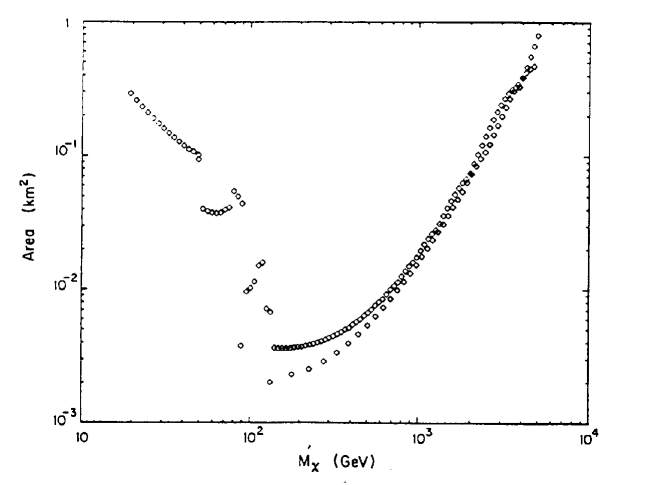
Figure 8: Detector effective area required to reach a one event per year level sensitivity. M_χ is the neutralino mass. More details can be found in [17]

  This calculation has been performed in [8, 17, 37] in terms of the sensitive area required to detect a 4 standard deviations signal as a function of the neutralino mass. The results of this calculation shows (see fig. 8) that a detector with an area of 1 km² running for one year would be sensitive to a range of neutralino masses extending up to a few TeV.

• Atmospheric neutrinos:
  

  For all subjects described above, the atmospheric neutrinos constitute a source of background which is suppressed by using an energy threshold of $\approx$ 10  TeV. Nevertheless, atmospheric neutrinos may be an interesting subject of study by lowering the energy threshold to $\approx$ 10 GeV.

  In this case, the analysis of the angular distribution of muon neutrinos will allow the study of the flux as a function of the thickness of matter crossed through the Earth which varies from a few tens of km to 13 000 km depending on the zenith angle. This should allow to look for neutrino oscillations in a domain of the oscillation parameter space where Kamiokande has shown some evidence of such an effect [38]. However, even if atmospheric neutrino oscillations were confirmed by SuperKamiokande [39], it would be useful to cross-check such a result using a different technique.

1.2 Scientific motivation in Sea Science and Geology

Several fields of science are interested in long term measurement in deep sea environment, some need real time information (e.g. seismology), some do not and there are many efforts going on in this direction.

At the time being, the foreseen programme deals mainly with the carbon cycle, with current measurements and with geological measurements.

It is certainly not a complete list of what can be done and future developments may enlarge the scope of these studies.

1.3 The km-scale detector

In order to observe with relevant statistics the diffuse flux of neutrinos from AGNs and from point sources, and to be sensitive to neutralinos with masses above 1 TeV, a km-scale detector is necessary. We believe that the technology needed to build such a detector is available. The first phase of the ANTARES project, described below, aims at demonstrating the feasibility of such a detector.

2 Neutrino telescope concept

2.1 Basic principle

The detector consists of a 3-dimensional array of optical modules (OMs) immersed in the deep sea, 100 m above the sea bed. Figure 9 shows two possible arrays, the first one with a limited number of OMs will have a higher muon energy threshold than the second one which has more OMs. An OM is made of a photo-multiplier tube (PMT), its electronics and power supply housed in a pressure resistant glass sphere. We have considered 8 and 15 inch PMTs with hemispherical photo-cathode. Each PMT is shielded against the Earth magnetic field by a high permittivity metallic cage.

The OMs are hooked to a mechanical structure which ensures the stability of their relative positions in water.

A muon neutrino converts to a muon via a charged current interaction with a nucleon of the rock or the surrounding sea water. Cherenkov light is emitted in the sea water by the muon and then is detected by the OMs. The measurement of the arrival time of the light over at least five OMs allows the reconstruction of the muon direction. The amount of collected light allows to estimate the muon energy which is a lower limit of the neutrino energy.

Optical beacons consisting of glass spheres housing blue GaN LEDs allow a local time and amplitude calibration of the OMs. However, to be able to perform a global time calibration of a large scale detector, a light source such as a YAG laser is required, because of its greater light yield.

There are different ways of arranging physically the photo-multipliers (orientation, pairing…). A final choice will result from optimization of efficiency, resolution and cost.

Different schemes for the data transmission can be considered [40, 41]. For the readout of the optical modules one can have a cluster of about 10 OMs grouped around a local controller. Most of the signals that an OM will detect will consist of single photoelectrons (SPEs). These SPEs are mostly caused by light emitting background processes such as beta decays of ⁴⁰K or bioluminescence. For ⁴⁰K the typical counting rates have been measured (see optical background measurements in section 3.1.1) to be about 60 kHz (20 kHz) at the 0.5 (0.3) PE level with a 15^′′ (8^′′) photo-cathode Hamamatsu PMT. In order to reduce this rate to about 1 kHz, PMT signals can be sent to the controller which elaborates a local coincidence between neighboring PMTs and triggers the digitization of the signals. The digital information is transmitted through several network nodes in the array to a terminal node. With such a scheme using front-end trigger and digitization, the data flow of a km-scale detector can be handled with conventional techniques such as coaxial cables and Ethernet protocol. The terminal node is connected to an electro-optical cable bringing the power and slow control commands from the shore. In the terminal node the digital information modulates the light output of laser diodes. This light is then transmitted to the shore via optical fibres.

2.2 Status of other projects

• AMANDA:
  

  The AMANDA collaboration intends to build a neutrino telescope in the Antarctic ice cap [2]. Strings of OMs are buried in holes drilled in the ice.

  The AMANDA collaboration has already deployed four detector strings at a depth of 1 km at the South Pole; during the 1995-1996 and 1996-1997 campaigns, they extended the depth to 2 km with an overall number of optical modules greater than three hundred. The analog signals are sent to the surface via coaxial cables (or twisted pair cables), which also supply the high voltage.

  Compared with a deep-ocean site, the ice provides a stable platform for safe deployment as well as a natural mechanical support for the detectors. The counting room can be installed at the surface above the detector thus simplifying the power and data transmission. The ice is a very pure and transparent medium. It is also free of radioactive elements such as ⁴⁰K as well as bioluminescence.

  However the ice medium has some drawbacks. Impurities such as air bubbles are trapped in the ice crystal lattice, causing the light to scatter. After several scatterings, the direction of the photons is randomized isotropically. The measured scattering length $\Lambda=\lambda/(1-<\cos\theta>)$ ($\lambda$ is the scattering length between two diffusions, $\theta$ is the scattered angle) ranges from 20 cm at 1000 m depth to 25 m (see for example [42]) at 2000 m depth. The depth in the ice is limited to about 2500 m while one may go deeper in the ocean. Due to its location at the South Pole, only the northern sky can be observed.

• BAIKAL:
  

  The BAIKAL collaboration has deployed an array of 96 OMs at 1 km depth in Lake Baikal [3, 43]. The deployment is performed in winter from the frozen surface of the lake. In order to suppress a background rate of tens of kHz in each OM from ⁴⁰K and bioluminescence in the lake, they pair OMs and look only at coincidences. The counting rate is reduced to a few hundred Hz. Half the OMs point upwards to achieve the same acceptance over the upper and lower hemispheres.

  The array of 36 OMs has been operating since April 1993, recording more than 6.5 10⁷ muons in one year. They have reached a record up/down rejection ratio of 10^-4 and, according to their Monte Carlo, will reach 10^-6 (atmospheric neutrino level) when they deploy their full complement of 200 OMs. With their 96 OMs, they should identify 1 to 2 upward neutrinos events per week.

• DUMAND:
  

  DUMAND has been a precursor in the field and they have studied many aspects of the problems [4]. A lot of their experience has to be taken into account.

  A recent SAGENAP report [5] has recommended DUMAND to be terminated.

• NESTOR:
  

  NESTOR is planned to be installed at a depth of about 3.8 km depth in the Mediterranean sea [6]. At this depth, the down-going muon flux is about 10⁴ times the up-going muon flux from atmospheric neutrinos, while it is 10⁵ - 10⁶ for AMANDA and BAIKAL. Half of its optical modules will point upwards. NESTOR is designed to have a higher number density of OMs in the central volume, to enable local coincidences on lower energy events.

  The mechanical structure of NESTOR is a 12 floor tower, each floor composed of a titanium star supporting a hexagonal array of OMs at the ends. Electronics is housed in a central titanium sphere on each floor. FADCs and memory operating at 300 MHz digitize the OMs signals and digital data are transmitted to the shore via a 12 fibre electro-optical cable. Each fibre is connected to a floor.

  Since 1989, many tests have been performed. The first tower is expected in the near future. A further phase includes the deployment of seven towers.

Presently, both the AMANDA and BAIKAL experiments have demonstrated their ability to deploy optical modules using ice as a support. However, better optical properties of the transparent medium and a deeper installation justify the need for a deep sea detector.

3 R & D Programme of ANTARES

The feasibility of the deployment and operation of a large detector in the deep sea needs to be demonstrated. Scientists of other fields have deployed acoustic detectors connected to the shore and used them reliably for many years. We intend to built a demonstrator which will prove the feasibility and will allow us to estimate the cost of a large scale detector. In order to ensure that the exercise is meaningful, we must only use techniques that can be extrapolated to a km-scale detector.
The ANTARES programme can be divided into 3 stages, which will be discussed in detail below:

1. deployment of simple strings (these operations have already started);

2. deployment of a string connected to the shore via an electro-optical cable;

3. deployment of several strings and their submarine electric interconnection (demonstrator).

For the completion of these stages, we have asked for the support of experts. We have started a collaboration with IFREMER and Centre d’Océanologie de Marseille (INSU) as well as CSTN, France Télécom Câbles, CTME…

More specifically, not only the know-how is requested, but also the availability of ships and submarines (IFREMER owned submarines: Cyana, Nautile and ROV 6000; dynamical positioning ships which are needed should be available).

The optical module, the data transmission, the trigger and the slow control of the experiment are under study. In general, quality assurance will be pursued.

The geometrical arrangement of the array of optical modules needs to be studied in order to optimize the effective area of the detector, the angular resolution and the rejection against down-going muons.

Site studies including water transparency, optical background and bio-fouling measurements have already been started and need to be continued. All the tools for site tests are either completed or in construction and in this first phase of operation we have started to learn:

• how to build strings of detectors,

• how to deploy and recover them,

• how to handle difficulties associated with deep sea operations.

3.1 Site studies

3.1.1 Quality of a site and measurements

Many different criteria have to be looked at before choosing a site for the deployment of a large-scale detector:

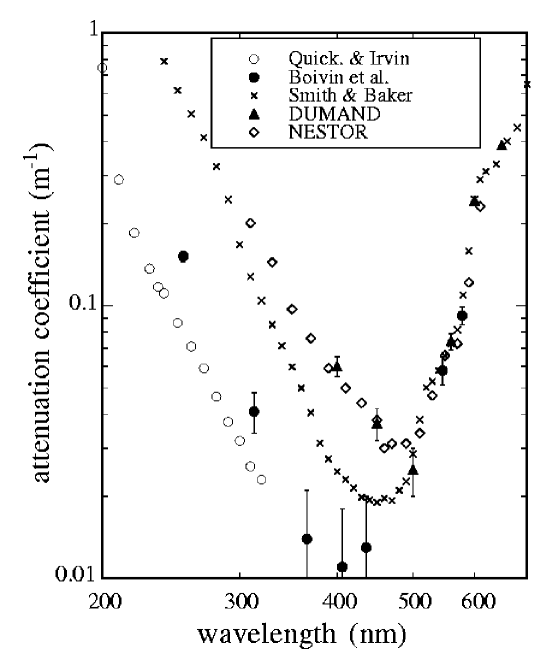
Figure 10: Attenuation of light in sea water as of function of wave length [42].

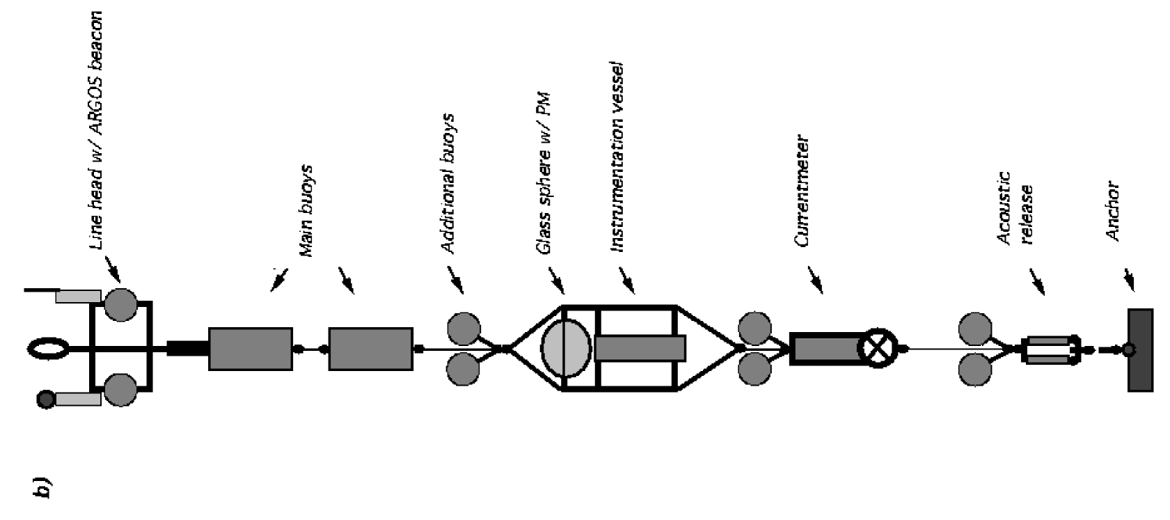
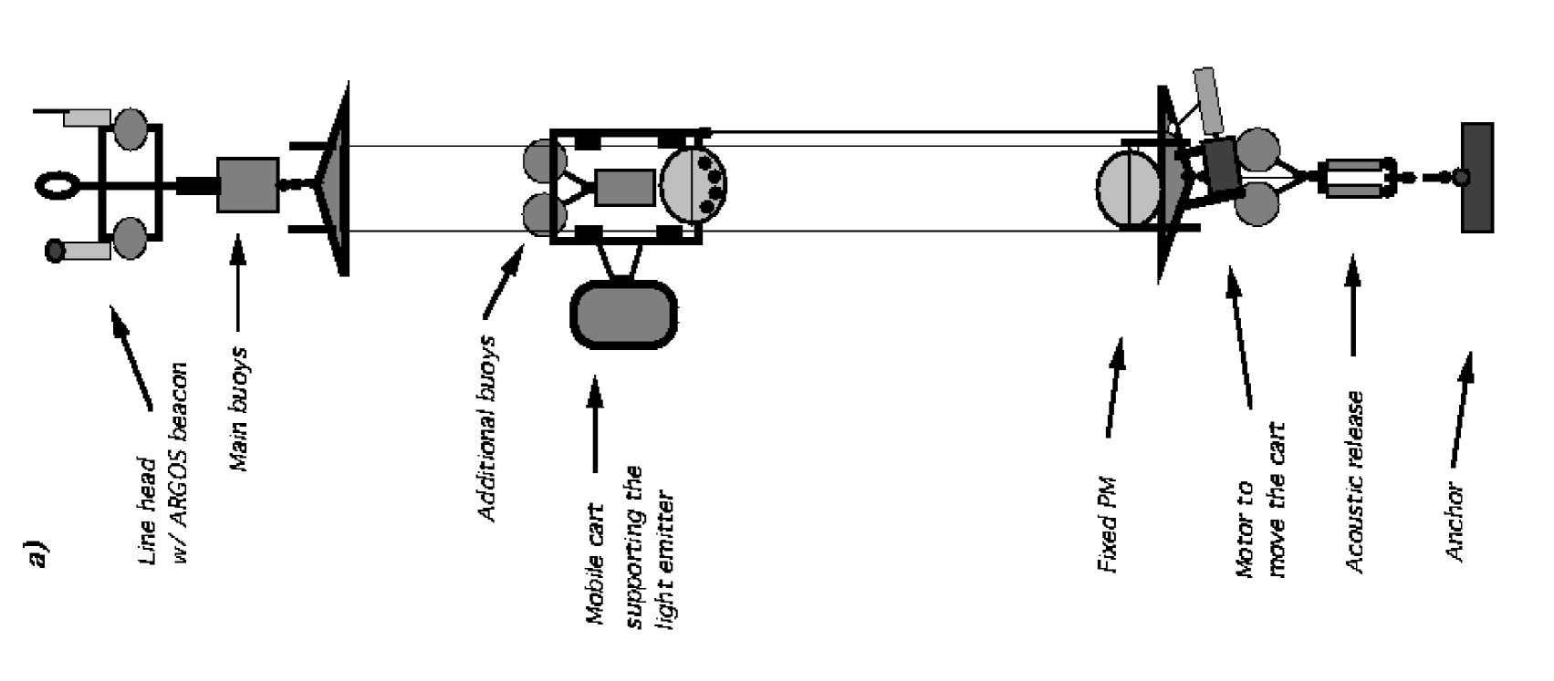
Figure 11: Schematic mooring lines to measure water transparency (a), optical background (b), biofouling growth (c)

1. Water quality:
   The sensitivity of the experiment will depend on the water transparency and the light scattering at large angles. The knowledge of the dependence of these two parameters as a function of the wavelength is required. These measurements are delicate as they need to be made in-situ with a 30m long measurement system with well characterized optical sources at different wavelengths. Some measurements by DUMAND and NESTOR exist (figure 10). A sketch of a design of our water transparency measuring device is shown in figure 11a.

2. Water depth:
   The water above the detector is a natural shield against atmospheric muons. The rate of down-going muons drops by a factor 10 going from 2500 to 4400 m. Figure 6 shows the rate of muons induced by atmospheric neutrinos and of direct atmospheric muons for an undersea depth of 3000 m.

3. Optical background:
   ⁴⁰K dissolved in salt water decays emitting electrons with an energy spectrum up to 1.3 MeV. Each electron produces 5 Cherenkov photons on average in the wavelength sensitivity window of the PMT. This gives rise to a photon flux of about 100 cm^-2s^-1 for a 50 m water attenuation length. This light emission is very likely to be site independent in the Mediterranean. On the other hand, bioluminescence (light emitted by a wide range of sea animal species) is time dependent and also site dependent. Bioluminescence in the deep sea is not well known and one should measure the time structure of the emitted light as well as spatial correlations. Those measurements are currently under way, see figure 11b. The first measurements have been done in October 1996 and in January 1997 at a depth of 2400 m about 25 km off-shore from Toulon (see 42^∘50’N-6^∘10’E in fig. 12).

4. Bio-fouling:
   Deep sea bacteria have the tendency to colonize the surface of immersed objects where they gather to form a sticky bio-film and make sediments hold on to it. This process is called bio-fouling. The speed of formation of the bio-fouling is site dependent. It may affect the transparency of the optical module in the long term. The rate of accumulation has to be measured at the site and anti-fouling solutions have to be investigated. Sea science physicists are proposing different practical ways. Collaborations with EEC partners of the Bio-film Reduction on Optical Surfaces programme has started and measurements using the line described in figure 11c are under way.

5. Deep sea currents:
   Currents have to be taken into account in the mechanical design of the detector. Currents are changing during the year, so they have to be measured on a year scale over the vertical range covered by a future detector. This will be done in collaboration with sea science specialists.
   Benthic storms can generate very high currents. The rate at which they have occured in the last 500 years can be deduced by geologists from a campaign of observation.

6. On shore station:
   Issues such as:

   • lab space,

   • pier availability,

   • ship and submarine availability,

   as well as general support have to be considered.
   The cost of access to these supports is site dependent and has to be taken into account in the cost evaluation of the project.

3.1.2 Test site

To test and implement the feasibility studies, the environment of a site is even more critical. We have started to use a site in the Toulon area (off-shore from La Seyne) at a depth around 2400 m (see 42^∘50’N-6^∘10’E in fig. 12). This site has several environmental advantages:

• IFREMER has a laboratory at La Seyne with piers, ships and submarines. A civilian ship (supply-type with dynamical positioning) is also available.

• France Télécom Câble ship is based there.

• INSU-CNRS have three ships which can be used in this area.

3.2 Mechanical handling of the detector: deployment, recovery and positioning

3.2.1 General remarks

The detector is an array of optical modules deployed close to the sea bottom. The physics requirement (muon threshold, up/down discrimination, calorimetry measurement…) will constrain the geometry of the array. Different geometries such as strings and more elaborate structures are shown in figure 9. We will have to deploy a substructure of this detector alone and with an electro-optical cable connected to it. One must also be able to make electrical interconnection of the many substructures and be able to recover part of the detector for servicing. A large scale detector with one electro-optical cable per substructure is unrealistic in terms of cost, deployment and recovery. However, a few electro-optical cables for the whole detector are required to handle the rate and to insure redundancy.

We will focus, in the present phase of the project, on a simple string-like substructure of optical modules a few hundred meter high equipped with a few tens of photo-multipliers. More elaborate substructures will be thought of for the future.

As we intend to keep the detector under water for several years, a special attention to corrosion problems will be given with the help of our IFREMER collaborators and quality assurance procedures will have to be set.

The detector as a whole should be aligned and the relative position of the different optical modules has to be monitored with an accuracy of 20 cm (see 3.2.4).

3.2.2 Step one: deployment and recovery of an elementary substructure

We will work on a simple substructure made of one string equipped with 20-30 optical modules and all the cables and the containers needed for the normal operation of the optical modules. We intend to use a string having all the complexity of a final substructure even if all the photo-multipliers and all their associated electronics might not be installed.

Vertically erected by its own buoyancy, the string is anchored on the sea bottom by a suitably dimensioned ballast. A schematic drawing is shown in figure 13. Apart from the optical modules, the string includes also current-meters, tilt-meters, accelerometers and compasses to learn about its dynamical behavior during deployment, operation and recovery.

The anchoring system should also keep in position the electro-optical cable connected to the shore, which delivers the necessary power and ensures the data transmission through optical fibres. It has to be designed in such a way that recovering and re-deployment of the structure is feasible.

Deployment and recovery in the deep sea are difficult operations. The complexity is increased by the electro-optical cable handling. It should be in principle possible to extrapolate the procedure routinely used by scientists deploying acoustic detectors at depth.

We consider this phase as a major step toward the km-scale detector. This step includes setting up a shore station (at Les Sablettes at La Seyne using the France Télécom Câbles terminal) and installation of acoustic beacons for the positioning of the string.

3.2.3 Step two: installation of a three dimensional array

A possible set-up of the demonstrator is shown in figure 14. Whatever a final choice for the substructure may be, one is faced with the under-water interconnection of different substructures. Indeed, schemes considering one electro-optical cable per substructure or all the interconnections made before a deployment of all the substructures at once, are unrealistic and cannot be extrapolated to a large scale detector.

In this step, one has to test the submarine connection. From the existing know-how, it is much easier to think in terms of electric connection than in terms of optical connection.

Some electric submarine connectors exist. We will have to check if they match our needs, in particular in terms of lifetime. Other connectors can be considered using an electro-magnetic coupling but they still have to be developed.

Following the advice of IFREMER experts, we will use a manned submarine (e.g. the Cyana which can be operated down to 3000 m) to start with, and once experience is gained, the submarine will be replaced by a remotely operated vehicle (ROV) which can be operated down to 6000 m.

The laying out of an interconnecting deep sea cable has to be carefully prepared. Preliminary work will start in 1997 and operational tests are expected in 1998.

Once one knows how to install substructures and how to interconnect them, one should be able to build a large scale detector.

3.2.4 Positioning of the optical modules

We need to know the relative position of the optical modules within 20 cm. This corresponds to the precision one can expect for the relative timing of photo-multipliers with a few photoelectrons. The angular resolution of the detector depends on the timing accuracy.

This can be achieved in principle with a triangular sonar base and acoustic detectors. Such a system is under study.

• The time resolution is proportional to the sonar frequency, so a high frequency is favorable. However, the sound wave attenuation length is proportional to the second power of the frequency and the power to be supplied increases also with frequency. A solution has to be defined and tested.

• The geometrical implementation of sonars and hydrophones, as well as the number of hydrophones needed for a given structure, should be optimized . The help of tilt-meters and compasses may decrease the number of hydrophones required well below one per optical module.

We plan to take advantage of the know-how of different groups working in the field. There may be alternative solutions to internal alignment. For example, a pulsed light source could in principle achieve the same goal. It remains to be proven and compared. One also has to get an absolute positioning of the whole detector to be able to point to individual sources. Solutions exist with acoustic devices connected to surface detectors coupled to differential GPS.

3.2.5 Mechanical studies of substructures

We have listed some of the problems which have to be taken care of in the construction of the substructures (corrosion, current effects, deployment…). We will make simulations and tests with mock-up and existing strings to understand the behavior of detectors and structures exposed to the deep sea current and to local sea conditions when the structure is deployed. We have already acquired experience from the first series of tests we have performed.

3.3 Optical modules

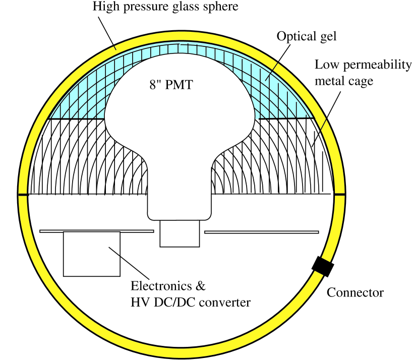
Figure 15: Optical module cross-section.

An optical module consists of a pressure-resistant glass sphere housing a photo-multiplier embedded in silicon gel to ensure a good optical coupling. A high permittivity alloy cage surrounds the tube, shielding it against the Earth magnetic field (see fig. 15). A DC/DC converter supplying power to the PMT is also included in the sphere. Signal outputs, HV monitoring, etc. are sent through water and pressure-resistant connectors to the outside world. A later version using digital read-out electronics will also house the front-end digitizer board described later in this document.

The choice of photo-multiplier will be based on several parameters:

• the photo-cathode size, to maximize sensitivity;

• the anode pulse shape, which has an impact on trigger system;

• the overall quantum efficiency, as well as the response uniformity and the sensitivity to residual Earth magnetic field (once the PMT is shielded);

• the Transit Time Spread at the single photo-electron (SPE) level, which contributes to the event reconstruction efficiency;

• the SPE pulse height and energy resolution;

• the linearity and dynamic range. The Cherenkov light detected by an optical module will vary from a SPE level to an amount causing saturation of the anode signal, depending on the distance to the trajectory, on the energy of the muon and on the proximity of the hadronic shower. Output signals from one or several intermediate dynodes will be needed to cover the whole dynamic range;

• the dark current level, which affects the coincidence rates between PMTs;

• the rate of pre- and after-pulses, which can mimic e.g. signals from muon bundles.

In order to characterize optical modules we have set up various testing facilities.

A test bench consisting of a couple of dark boxes with and without magnetic shields, in which the PMTs are exposed to homogeneous illumination coming from red, green or blue LEDs or very fast solid state laser pulsers (to measure time characteristics). The main PMT characteristics are measured and compared: dark count rate and spectrum, rate and time structure of pre- and after-pulses, signal pulse shape, photo-multiplier gain, SPE resolution, Earth magnetic field effects, magnetic shielding efficiency, SPE transit time spread, overall relative efficiency, linearity and dynamic range, ….

Another dark box equipped with a mechanical system allowing a blue LED to scan the active area of the photo-cathode is used to control the homogeneity of the parameters listed above as a function of the position of the light spot on the photo-cathode.

A water tank is used to study the overall response of the optical module to Cherenkov light emitted by vertical cosmic muons in water. The module can be rotated around a horizontal axis, making it possible to measure the optical module response at different muon angles of incidence. This set-up has also been used in the 200 GeV M2 muon beam at CERN.

Several types of photo-tubes have been tested. We have extensively studied the performances of optical modules with Hamamatsu R2018-3 15^′′ photo-tubes. Such large area tubes fit well in the largest available pressure-resistant glass spheres (17^′′). However they show important drawbacks. The signal amplitude strongly depends on the distance to the photo-cathode pole of the photon conversion point. These PMTs were also shown to be sensitive to the residual Earth magnetic field. Some of these photo-tubes showed significant pulse shape variations even for a constant amplitude, and the dark noise rate has shown to be significant and very unstable in time. Moreover, the dynode structure seems to be too fragile to safely cope with the mechanical stress likely to occur during a deployment at sea.

Therefore, we have started to test existing commercial 8^′′ PMTs from Hamamatsu and EMI. First measurements indicate that they do not suffer from the same flaws as their 15^′′ counterparts. Hamamatsu R5912 (10 stages) and R5912-02 (14 stages) and EMI 9353KB (12 stages) and 9355KB (14 stages) are being tested and give satisfactory preliminary results, namely: stable behavior, low dark noise ($<$ 1kHz), good efficiency and homogeneity, good SPE resolution ($\approx$ 30%), good SPE time resolution ($<$ 3 ns FWHM) and no measurable effect of the residual Earth magnetic field. 8^′′ PMTs are used extensively in site measurement tests, so some experience on their behavior in-situ has been gained.

3.4 Data transmission, trigger and acquisition

Dedicated electronics and data acquisition has been developed for the stand-alone test programme.

For the demonstrator, analog and digital data transmission schemes are both being studied. For the first structure that will be deployed and connected to an electro-optical cable, we plan to use an analog transmission. Its intrinsic robustness makes it easy to implement and suited to our short term needs. However, we have reached the conclusion that only a digital data transmission can meet our requirements for a km-scale detector.

3.4.1 Electronics and acquisition system of the stand-alone tests

The electronics and acquisition system required for our stand-alone tests have been developed around a MBX 9000 acquisition board from MII, equipped with a 16 MHz MC68306 processor from Motorola, one Mbyte of PROM and up to two Mbytes of RAM for data storage. Digital and analog I/O’s including two serial links are available for dialogue with each specific equipment such as current-meter, acoustic modem and the extension board that holds the electronics needed for each test. A Unix-like real-time operating system is running on the processor. The acquisition is written in C. A configuration file describing the test sequence, is read by the acquisition program at the startup of the processor.

3.4.2 The electro-optical cable

We have the opportunity to use an already existing cable that is equipped with four mono-mode fibres. The measured attenuation is 0.33 dB/km at $\lambda$ = 1310 nm. The required cable length to reach the test site is around 40 km.

3.4.3 Analog link

Up to now, we have studied an analog transmission scheme using direct modulation of distributed feedback (DFB) laser diodes with frequency modulation of several carriers which are multiplexed (FDM). We tested two systems, a 3-channel multiplexing prototype built by IDREL, coupled to a wide-band ORTEL optical link and a THOMSON 4-channel prototype.

The 3-channel prototype by IDREL, with carriers at 1.35, 1.50 and 1.65 GHz was tested and improved. With a 35 km fibre link (0.36dB/km), the linearity was measured and the dynamic range is $\simeq$ 30. The time dispersion is $\leq$ 1.3 ns (RMS). If we use the available cable of 40 km, with a stronger attenuation (0.5dB/km) the dynamic range would be strongly diminished ($\simeq$ 3).

The THOMSON prototype TER7000 transmits on four carriers, between 300 and 900 MHz, and four analog channels with 50 MHz BW each. The measured performance with a 35 km fibre is a dynamic range of 40 to 50 and a time dispersion of 1.3 ns (RMS).

Using the available cable we are considering the transmission of eight PMT signals using direct modulation and a simple method of mixing, without RF multiplexing.

Increasing the number of frequency-multiplexed channels appears to be non trivial. To date, a digital solution seems to be the only way to meet the requirements of a km-scale detector.

3.4.4 Digital link

A possible digital architecture for a large scale detector could be organized as a tree-structured network of MCMs (Main Control Modules), SCMs (String Control Modules), LCMs (Local Control Modules) and DOMs (Digital Optical Modules) (see e.g. the LBNL-JPL group proposal [44]). The MCMs would be connected to the shore via electro-optical cables. Interconnections between control modules at the same level in the network hierarchy would ensure a path redundancy for data/control information.

A possible approach to digitize the signals at the optical module level is to have LCMs connected to several DOMs via bidirectional links. Each DOM produces a local trigger which is transmitted to the LCM. A higher level trigger produced in the LCM is sent back to the DOM’s in order to enable digitization and data transmission.

• The Digital Optical Module (DOM):
  In [44] it is proposed to develop a DOM based on a ASIC designed at LBL, the Analog Transient Waveform Recorder (ATWR).

  We are developing a similar architecture, in a circuit called Analog Ring Sampler (ARS). The ARS ASIC consist of an array of 128 capacitor cells which samples and memorizes analog input signals. The sampling frequency is adjustable from 300 MHz to 1 GHz. The ARS has five channels of 128 cells, one channel for the signal coming from the PMT anode, two channels for the signals coming from two intermediate dynodes, one channel dedicated to time stamping in which a stable 20 MHz clock is recorded and the last channel being used for accurate pedestal subtraction.

  In acquisition mode, the ARS is constantly sampling the PMT signals as a ring memory. When the PMT signal crosses a comparator threshold corresponding to a fraction of SPE the ARS stops overwriting its cells. The comparator signal is sent to the Local Control Module (LMC) where the trigger is built.

  In order to reduce the amount of data to be transmitted, pulse shape discrimination (PSD) is performed in parallel to trigger building. The decision is made whether to provide only time and charge (SPE Mode) or to fully digitize pulse shapes departing from SPE (Waveform Mode).

  The shape discrimination consists of a threshold comparator, a time-over- threshold comparator and a multi-pulse detector in order to recognize three kinds of shapes: high pulses, long pulses and multiple pulses.

  The motherboard, inside the DOM, supports two channels (ARS) in “flip-flop” operation, to reduce dead-time. It also drives the power supplies and surveys the current, voltage and temperature, generating an alarm signal if necessary. It receives the clock from the LCM and supports the slow control.
  

• The Local Control Module (LCM):
  The LCM is the next node in the digital network of the detector array. It is connected to about 10 DOMs on one hand, to the next digital node (e.g. String Control Module) on the other hand. It takes care of power distribution, slow control commands and data, trigger building and formatting and transmission of DOM data to the SCM.

  Any DOM which is locally triggered sends a coincidence request to the LCM. The LCM looks for a time coincidence with a request from any of the other DOMs connected to it and sends back a data request signal to the DOMs involved. The data are then digitized and sent to the LCM. A scheme where the DOMs are grouped in close clusters (e.g. pairs or quadruples) allows tight time coincidences. The accidental coincidence rate coming from ⁴⁰K can be kept around 100 Hz and the system can cope with up to a few 100 kHz bioluminescence bursts before suffering from significant dead time.

  The front end PSD ensures that the data flow will be minimal. In SPE mode, an event represents about 30 bytes of data. In Waveform mode (e.g. 1$\%$ of the time), it goes up to 600 bytes. The average data flow will not exceed 50 kbyte/s per LCM. This allows the use of Ethernet(-like) protocols for the detector network.

3.5 Slow Control

Optical modules (PMTs voltages, temperatures), calibration, positioning systems and sensors for detector geometry together with sea parameters are controlled and read out by the slow control system which gives a user in the shore station all the needed graphical and numerical information to monitor and control the detector.

The slow control system will be based on an industrial field-bus network technology providing reliability, robustness and scalability features to such an embedded detector control. The bandwidth of these field-buses will fit our future system extensions (sensors, control devices). The link between the undersea part of slow control and the shore station will be done via the electro-optical cable. An interface using an acoustic modem will provide the user means for a stand-alone (without connection to shore) pre-diagnosis of the slow control system.

3.5.1 Slow Control network

To transfer data from the sensors and control-command messages to the optical modules (OM), we will use an industrial field-bus network technology called WorldFip designed in the early 90’s to cope with sensors and actuators control in a factory environment. The main features of WorldFip are :

• Deterministic field-bus, the communication protocol used in WorldFip allows a mix of periodic and aperiodic data transfers. In the first case, the time schedule of periodic variables is warranted.

• High speed sensor/actuator communication (32 kb/s, 1 Mb/s, 2 Mb/s)

• Long distance connection between WorldFip nodes (up to 1 km at 1 Mb/s)

• Redundancy, WorldFip support bi-medium connection on two different shielded copper twisted pair. A switch to the best medium is automatically done by the WorldFip protocol chipset.

• Reliable bus arbitration policy based on multiple bus arbiter modules on the same WorldFip network.

We increase the robustness of the slow control architecture by segmenting the network by using an active network star repeater. In this architecture, each LCM container of the string is directly connected to the main Slow Control data acquisition system. A test bench for WorldFip network implementation evaluation is already setup using two PC’s and WorldFip to PC interfaces from CEGELEC (FullFip and MicroFip).

3.5.2 Slow Control bridge system

The Slow Control sensors (attitude and environment sensors) will mainly be read through serial interfaces (RS232 and RS485) while the Optical Modules (OM) will be locally controlled by a micro-controller (for temperature, DC, calibration LED) communicating through RS485 differential lines. The interface between these serial lines and the WorldFip network is performed by using a MBX9000-40 acquisition board (see paragraph 3.4.1) which can support 8 serial lines and is interfaced to WorldFip network (add-on module). One serial line will be dedicated to the string geometry sensors readout (tilt-meters, magnetic field..) and the others will be individually connected to the optical modules. One bridge system is included in each LCM container of the string.

3.5.3 Slow Control acquisition system

The slow control data acquisition (DAQ) system is build around a G96 module with a Motorola 68k processor running an embedded real-time OS9 operating system. The Gespac G96 bus connects this processor module to a G96 bi-medium WorldFip module (linked to the WorldFip active star repeater) and the I/O modules controlling energy distribution. This DAQ system is located in the Main Electronic Container located at the bottom of the string. An electro-optical cable connects this embedded Slow Control DAQ system to the shore station which receive the Slow Control data and provides a user interface for the Slow Control system.

4 Simulation and detector optimization

4.1 General remarks

A Monte Carlo simulation of our detection system is necessary to give us a way to study how to:

• optimize the geometry of the detector,

• adjust trigger schemes,

• tune track reconstruction algorithms,

• estimate energy resolution,

• investigate effects of backgrounds:

  • atmospheric $\nu$’s and $\mu$’s,

  • ⁴⁰K and bioluminescence,

• estimate the detector sensitivity to various neutrino sources.

The Monte Carlo program has to deal with Cherenkov photons generated by neutrino induced muons together with the electromagnetic and hadronic showers they caused while traveling through the detector and its neighborhood. The program simulates the propagation of these photons in water and the signal they induce on the 3-D matrix of optical modules the detector is made of. Because the number of secondary particles accompanying the primary muons increases dramatically with energy, a full simulation à la GEANT (which needs anyway to be modified to be reliable above 10 TeV) becomes quickly CPU-time prohibitive as energies of order a few TeV are reached (see figure 16). As large samples of events are needed in order to study resolutions and efficiencies, two approaches are currently being investigated:

• a parameterization of the Cherenkov light distributions of electromagnetic and hadronic showers, as pioneered by SiEGMuND (Baikal collaboration) [45],

• generated Cherenkov light look-up tables, as used in RAVEN (AMANDA) [46] and the KM³ simulation programs [47].

4.2 Geometry

Variations of geometrical parameters like the number of PMTs, their density, their spatial distribution, their size and type, the distance between groups of PMT, are being studied in order to optimize trigger and reconstruction efficiencies as well as angular and energy resolution. The detector effective area A_eff is defined as A${}_{eff}=f\cdot S$, with $S$ the surface inside which muons are generated uniformly and $f$ the fraction of events that pass the trigger and/or give a successful track reconstruction. It depends strongly on the requested angular reconstruction accuracy and increases substantially with energy.

4.3 Trigger studies

Several trigger configurations will be necessary to cover different physics channels of interest. For the demonstrator, the trigger will be an easy problem to solve. For a large scale detector, the main emphasis at the beginning will be put on neutrino induced muons with energy deposition all along their trajectories. Other more difficult channels as supernovae neutrino bursts and “double” bang structures for $\nu_{\tau}+N\rightarrow\tau+X$ events will be studied later. Most of these channels satisfy the simple criterion of a minimal number of photo-multipliers (PMT) above a threshold set below 1 photo-electron (PE). The goal is to trigger efficiently on muons in the largest possible volume for a given cost of the detector.
The main optical backgrounds (bioluminescence and natural radioactivity) are uncorrelated and mostly contribute to 1 PE signals, so the trigger can be designed with tight coincidences and/or a signal threshold greater than 1 PE. We need to quantify the trigger efficiency for a minimal number of hit PMTs estimating the detector effective area by computations based on Monte Carlo simulations. Several PMT configurations are currently under study.

4.4 Muon track parameters

• Muon track reconstruction:
  The muon which triggered the system has to be reconstructible (i.e. we need sufficient information to efficiently determine the muon direction with a good enough angular accuracy). The effective area used to evaluate the different geometric configurations has to be corrected for reconstruction efficiencies.
  Several reconstruction algorithms, all based on the characteristics of Cherenkov light emission, are currently under study. A muon track is characterized by five parameters (one space point and two angles), so at least five hit PMTs are needed. For a given track, the arrival time of the Cherenkov light on PMT $i$ can be calculated as:

  $$c~{}t_{i}=L_{i}+d_{i}\tan\theta_{c}$$

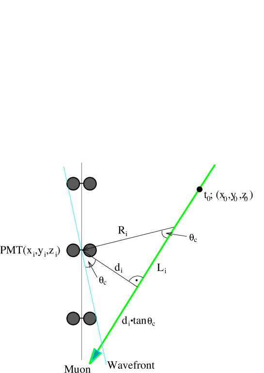
Figure 17: Track reconstruction principle.

  where $d_{i}$ is the impact parameter of the muon track w.r.t. the PMT, $L_{i}$ the distance between the track point at a distance $d_{i}$ from the PMT and the track point corresponding to the triggering time (t=0), $c$ the speed of light in vacuum and $\theta_{c}$ the Cherenkov angle (see fig. 17). The problem then boils down to a minimization of:

  $$\chi^{2}=\sum_{i}\frac{1}{\sigma_{t}^{2}}\left(t_{i}^{m}-t_{i}\right)^{2}$$

  with $t_{i}^{m}$ the measured arrival time of Cherenkov light on PMT $i$ and $\sigma_{t}$ the time resolution of the PMT ($\sigma_{t}=\sigma_{1PE}/\sqrt{N_{i}}$ with $\sigma_{1PE}$ the PMT time resolution for a 1 PE signal and $N_{i}$ the signal charge measured in units of PEs).

• Muon energy estimate:
  In the above expression, the charge of the PMT signals enter only indirectly through the time resolution. Actually, this extra information is complementary though it is more subject to big fluctuations. We reserve its use to select PMTs which are to be used in the fit and also to estimate the muon energy. A way to find the most probable energy of the muon could be to use a maximum likelihood method à la Baikal. They define a function:

  $$L(\log E_{\mu})=\prod_{i=1}^{N}W_{i}(E_{\mu},A_{i},R_{i},\theta_{i},\phi_{i})$$

  with $W_{i}$ the probability to observe an amplitude $A_{i}$ on PMT $i$ located at a distance $R_{i}$ from the muon trajectory and with angles $\theta_{i}$ and $\phi_{i}$ w.r.t. it if the energy of the muon is assumed to be $E_{\mu}$; N is the overall number of PMTs at a distance $R<R_{min}$ from the muon trajectory.

• Pending issues to be studied:

  • the impact of non-correlated backgrounds on the reconstruction efficiency and trigger rates, and the optimization of selection and reconstruction algorithms in order to minimize the effects of such backgrounds,

  • the reconstruction efficiency with emphasis on reconstruction errors. The issue here is to succeed in rejecting single downward going atmospheric muons as well as multiple downward going muons which, if too close in time, could fool the reconstruction algorithm and be taken as a single upward going muon. In this latter case, a shape analysis provided by a fast enough sampling of the PMT signals could prove to be very helpful,

  • the reconstruction efficiency for very high energy muons (PeV and above), for various geometries.

5 The ANTARES Collaboration

5.1 Collaborating institutes

The collaboration consists of groups of particle physicists and engineers from:

• CPPM Marseille (IN2P3-CNRS/Université de la Méditerranée):
  C. Arpesella, E. Aslanides, J.J. Aubert, S. Basa, V. Bertin, M. Billault, P.E. Blanc, A. Calzas, C. Carloganu, J. Carr, J.J. Destelle, F. Hubaut,
  E. Kajfasz, R. Le Gac, A. Le Van Suu, L. Martin, C. Meessen, F. Montanet, Ch. Olivetto, P. Payre, R. Potheau, M. Raymond, M. Talby, E. Vigeolas.

• DAPNIA-DSM-CEA (Saclay):
  R. Azoulay, R. Berthier, F. Blondeau, N. de Botton, P.H. Carton,
  M. Cribier, F. Desages, G. Dispau, F. Feinstein, P. Galumian, L. Gosset, J.F. Gournay, D. Lachartre, P. Lamare, J.C. Languillat, J.Ph. Laugier,
  H. Le Provost, D. Loiseau, S. Loucatos, P. Magnier, J. McNutt, P. Mols, L. Moscoso, P. Perrin, J. Poinsignon, Y. Sacquin, J.P. Schuller, J.P. Soirat, A. Tabary, D. Vignaud, D. Vilanova.

• Instituto de Física Corpuscular – CSIC-Universitat de València:
  R. Cases, J.J. Hernández, S. Navas, J. Velasco, J. Zúñiga.

• Oxford University – Physics Department:
  D. Bailey, S. Biller, B. Brooks, N. Jelley, M. Moorhead, D. Wark.

of groups of sea scientists from:

• Centre d’Océanologie de Marseille:
  F. Blanc, J.L. Fuda, L. Laubier, C. Millot.

• IFREMER:
  J.F. Drogou, D. Festy, G. Herrouin, L. Lemoine, F. Mazeas, P. Valdy.

of groups of astronomers and astrophysicists from:

• IGRAP (INSU-CNRS):
  Ph. Amram, J. Boulesteix, M. Marcelin, A. Mazure, R. Triay.

• DAPNIA-DSM-CEA (Saclay):
  Ph. Goret.

The collaboration has also the support of other organizations as France Télécom Câbles, CSTN, CTME.

Geophysicists have shown an interest to share some technological developments (IPG - Paris, Sophia Antipolis - Nice).

5.2 Schedule

The existing programme has been approved for the demonstrator implementation and will be performed over 1997, 1998 and 1999.

We would like to complete in the first year the apparatus dedicated to the site tests, then in the second year to have one string with an electro-optical cable and in the third year to complete the 3-dimensional demonstrator. In the same time, one should develop the tools for the next phase.

5.3 Enlargement of the Collaboration

New collaborators are needed, as soon as possible, to bring new ideas and to participate in these developments. There are lots of tasks which have to be achieved as in a standard particle physics experiment.

The collaboration is actually sharing the most urgent tasks and it has been decided to redistribute every year the responsibilities, to be able to take into account the changes in the collaboration.

After the completion of the demonstrator, we would like to build a km-scale detector step by step. The next stage may be a high muon energy threshold detector of a large effective surface with several hundred photo-multipliers. This stage can be achieved with new collaborators on a reasonable time scale.

APPENDIX
Neutrino-matter interaction

• The inclusive charged current cross-section for $\nu_{\mu}+N\rightarrow\mu^{-}+X$ is given by [29]:

  $$\frac{d^{2}\sigma_{\nu N}}{dxdy}=\frac{2G^{2}_{F}m_{N}E_{\nu}}{\pi}\frac{M^{4}_{W}}{(Q^{2}+M^{2}_{W})^{2}}\left[xq(x,Q^{2})+x(1-y)^{2}\bar{q}(x,Q^{2})\right]$$

  where $x=Q^{2}/2m_{N}\nu$ and $y=\nu/E_{\nu}$ and with $Q^{2}$, the square of the momentum transfer between the neutrino and muon, $\nu=E_{\nu}-E_{\mu}$ the lepton energy loss in the lab frame, $m_{N}$ the nucleon mass, $M_{W}$ the $W$-boson mass and $G_{F}$, the Fermi constant. For an isoscalar nucleon, in terms of valence ($v$) and sea ($s$) parton distribution functions:

  $$q(x,Q^{2})=\frac{u_{v}+d_{v}}{2}+\frac{u_{s}+d_{s}}{2}+s_{s}+b_{s}$$

  $$\bar{q}(x,Q^{2})=\frac{u_{s}+d_{s}}{2}+c_{s}+t_{s}$$

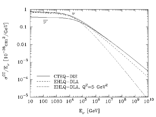
Figure 18: Energy dependence of the $\nu N$ and $\bar{\nu}N$ charged current cross-sections according to CTEQ3 and EHLQ parton distribution functions (taken from [29]).

  The energy dependence of the cross-section is shown in figure 18 (see ref. [29]).
  

  At low energies, the cross-section grows linearly with the neutrino energy:

  $$\sigma_{\nu N}(E_{\nu})\simeq 0.67~{}10^{-38}E_{\nu}[GeV]~{}cm^{2}$$

  $$\sigma_{\bar{\nu}N}(E_{\nu})\simeq 0.34~{}10^{-38}E_{\nu}[GeV]~{}cm^{2}$$

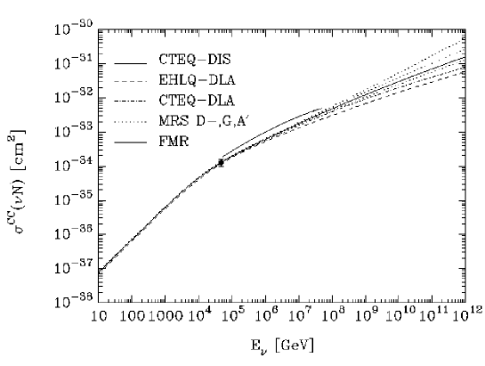
Figure 19: CC-cross section for $\nu_{\mu}N$ interactions for different sets of parton distribution functions. The data point corresponds to the average of measurements by H1 and ZEUS collaborations at HERA (taken from [29]).

  At energies such that $E_{\nu}\gg M^{2}_{W}/2m_{N}\approx 5$ TeV, the $W$ propagator limits the growth of $Q$ to $<Q^{2}>\sim M^{2}_{W}$ and makes the cross-section to be dominated by the behavior of distribution functions at small $x$ ($x\sim M^{2}_{W}/2m_{N}E_{\nu}<y>$).
  The H1 and ZEUS collaborations at HERA measured the proton structure function $F_{2}(x,Q^{2})$ via charged current $e-p$ scattering, for $Q^{2}$ in the range $[1.5,5000]$ GeV² with $x$ down to $3~{}10^{-5}$ at $Q^{2}=1.5$ GeV² and $x$ down to $2~{}10^{-2}$ at $Q^{2}=5000$ GeV² [48]. These measurements can be translated into a neutrino-nucleon interaction cross section at $E_{\nu}\simeq 50$ TeV and can also be used as a guide to extrapolate the parton densities beyond the measured ranges in $x$ and $Q^{2}$ required at even higher neutrino energies. Figure 19 shows the behavior of the interaction cross section of a $\nu_{\mu}$ with an isoscalar nucleon for different sets of parton distribution functions. At very high energy, the newly calculated cross section (see fig. 18) with CTEQ3-DIS [49] parton distribution functions, is more than a factor of 2 larger than the pre-HERA estimate calculated with EHLQ parton distribution functions.

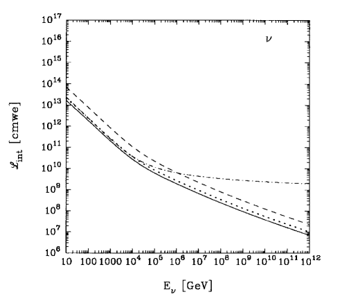
Figure 20: Interaction lengths for $\nu N$ interactions. When computed with the CTEQ3-DIS parton distribution functions: dotted line, CC-interactions; dashed line, NC-interactions; solid line CC+NC. The dot-dashed curve corresponds to CC-interaction with EHLQ unevolved ($Q^{2}=5$ GeV²) structure functions (taken from [29]).

• As the calculated cross section was underestimated at high energy, so was the attenuation of the neutrino flux in the Earth. Figure 20 shows the interaction length $\cal L_{int}$ of $\nu_{\mu}$’s on nucleon targets as a function of $E_{\nu}$. $\cal L_{int}$ is given by $\cal L^{-1}_{int}=N_{A}\sigma_{\nu N}(E_{\nu})$, where $N_{A}$ is the Avogadro number. At energies greater than $\simeq$ 40 TeV, the interaction length becomes smaller than the Earth diameter.
  

  The attenuation of neutrinos in the Earth can be described by a shadow factor $S(E_{\nu})$ given by:

  $$\frac{dS(E_{\nu})}{d\Omega}=\frac{1}{2\pi}\exp\left[\frac{-d(\theta_{z})}{\cal L_{int}(E_{\nu})}\right]$$

  where $d(\theta_{z})$ is the column depth of the Earth at zenith angle $\theta_{z}$.

• The energy loss of muons in matter is due to quasi-continuous (with small fluctuations) ionization processes but also to radiative processes (bremsstrahlung, pair production and photo-production) subject to big fluctuations (for a thorough treatment of the propagation of multi-TeV muons in matter see ref. [50]). The average loss can be expressed as:

  $$\left<\frac{dE(E_{\mu})}{dX}\right>=\alpha+\beta E_{\mu}$$

  where $\alpha$, representing the ionization contribution, is logarithmically increasing with energy. $\beta$ is the sum of the fractional energy radiation losses. For $E_{\mu}$ greater than the critical energy $\varepsilon=\alpha/\beta$, the radiation losses dominate. Bremsstrahlung and pair creation contributions to $\beta$ reach an asymptotic value at high energy, but it is not so for the photo-nuclear contribution which keeps rising with energy.
  If $\alpha$ and $\beta$ are taken to be energy independent ($\alpha\simeq 2.0~{}10^{-3}$ GeV cmwe^-1, $\beta$ = 3.9 10^-6 cmwe^-1 in rock so $\varepsilon\simeq 500$ GeV), then the range of the average loss for a muon of initial energy $E_{\mu}$ and final energy $E^{min}_{\mu}$ is given by:

  $$R_{<\Delta E>}(E_{\mu};E^{min}_{\mu})=\int_{E^{min}_{\mu}}^{E_{\mu}}\frac{dE_{\mu}}{\left<\frac{dE(E_{\mu})}{dX}\right>}\simeq\frac{1}{\beta}\ln\left[\frac{\alpha+\beta E_{\mu}}{\alpha+\beta E^{min}_{\mu}}\right]$$

  For $E_{\mu}\ll\varepsilon$, the range of muons is correctly reproduced by $R_{<\Delta E>}(E_{\mu})\propto E_{\mu}$ as ionization processes dominate.
  For $E_{\mu}\gg\varepsilon$, $R_{<\Delta E>}(E_{\mu})\propto\ln(E_{\mu})$. However, in this regime, the radiation losses dominate and because of their big fluctuations:

  • the average range $<R(E_{\mu};E^{min}_{\mu})>$ of the muons is smaller than the range of the average loss $R_{<\Delta E>}(E_{\mu};E^{min}_{\mu})$,

  • the width of the range distribution increases with energy,

  so the range of the average loss only poorly reproduces the actual range of high energy muons. In order to estimate the range of high energy neutrinos correctly, it is necessary to use a Monte-Carlo method to propagate them.

Two approaches can be followed to calculate muon rates $N_{\mu}$ in a detector:

• Analytically, the probability for a neutrino of energy $E_{\nu}$ to give a muon of energy $E_{\mu}>E^{min}_{\mu}$ in the detector is given by:

  $$P_{\mu}(E_{\nu};E^{min}_{\mu})=N_{A}\sigma^{CC}_{\nu N}(E_{\nu})<R(E_{\mu};E^{min}_{\mu})>$$

  where $<R>$ is the average muon range in rock.
  The rate $N_{\mu}$ of muons induced by an isotropic neutrino flux $\frac{dN_{\nu}}{dE_{\nu}}$ in a detector of effective area $A$ is given by:

  $$N_{\mu}=A\int d\Omega dE_{\nu}P_{\mu}(E_{\nu};E^{min}_{\mu})S(E_{\nu})\frac{dN_{\nu}}{dE_{\nu}}$$

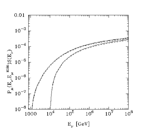
Figure 21: $P_{\mu}(E_{\nu};E^{min}_{\mu})S(E_{\nu})$ as a function of $E_{\nu}$ for $E^{min}_{\mu}$ = 1 TeV and 10 TeV respectively. The curves correspond to CTEQ3-DIS (solid) and EHLQ-DLA (dashed). (taken from [29]).

  where the shadow factor is integrated over the relevant solid angle. Figure 21 shows how the product $P_{\mu}(E_{\nu};E^{min}_{\mu})S(E_{\nu})$ evolves as a function of $E_{\nu}$ for two muon threshold energies $E^{min}_{\mu}$ of 1 and 10 TeV respectively.

• Using a Monte Carlo program in which a given neutrino flux is made to interact with the Earth, the induced muons are then propagated to the detector. It fully takes into account the large fluctuations occuring at high energy. This method was prefered to the analytical one to compute the rate results presented in section 1.1.4.

Energy	$\Phi_{0}$	Atm. neutrinos
threshold	(cm-2 s-1)	(cm-2 s-1 sr-1)
10 GeV	$1.3\cdot 10^{-13}$	$1.5\cdot 10^{-13}$
100 GeV	$1.2\cdot 10^{-13}$	$5.3\cdot 10^{-14}$
1 TeV	$6.6\cdot 10^{-14}$	$5.9\cdot 10^{-15}$
10 TeV	$1.5\cdot 10^{-14}$	$1.4\cdot 10^{-16}$

Table 1: Values of the neutrino induced muon flux $\Phi_{0}$ (see text) for different energy thresholds and for a differential spectral index $\gamma=2.2$ together with the flux of muons induced by atmospheric neutrinos averaged over the whole $2\pi$ downward hemisphere for the same thresholds.

Energy	${\cal L_{p}}$
threshold	(erg s-1)
10 GeV	8.3 1034
100 GeV	5.3 1034
1 TeV	4.8 1034
10 TeV	2.1 1035

Table 2: Luminosities of a neutrino source with a differential spectral index $\gamma=2.2$ located at a distance of 1 kpc that can be detected at a 5 $\sigma$ level (or 10 events per year) with an effective exposure of 1 km² year for different muon energy thresholds.

Source	Declination	Distance	${\epsilon}_{t}$	Expected	${\cal L}_{p}$
name	$\delta$	(kpc)		background	${\gamma}=2.2$
					(erg/s)
Pulsars
Crab	21∘	2	37.5%	0.4	5.1 1035
Vela	-45∘	0.5	100%	3.0	1.2 1034
PSR 1937+21	21∘	5	37.5%	0.4	3.2 1036
PSR 1953+29	29∘	3.5	31.3%	0.3	1.9 1036
PSR 1822-09	-9∘	0.6	55.1%	0.8	3.1 1034
PSR 1801-23	-23∘	2.7	64.0%	1.2	5.5 1035
Binary stars
Cyg-X3	41∘	10-12.5	16.5%	0.1	(2.9-4.5) 1037
Her-X1	35∘	5	25.3%	0.3	4.7 1036
Cyg-X1	35∘	2.5	25.3%	0.3	1.2 1036
SS433	5∘	5	47.2%	0.7	2.5 1036
Vela-X1	-40∘	1.4	81.7%	2.7	1.1 1035
SN remnants
Crab	22∘	2	37.5%	0.4	5.1 1035
1987A	-69∘	50	100%	2.6	1.2 1038

Table 3: Detectable proton luminosities for several known galactic sources. The detector latitude is $45^{\circ}$. ${\epsilon}_{t}$ depends on the declination $\delta$ of the source.

Model	$\cos\theta_{z}$	E${}^{min}_{\mu}$ = 1 TeV	10 TeV	100 TeV	1 PeV	10 PeV	100 PeV
	range
Atmospheric
ATM [25]	$[-.25,1.]$	16000	420	5.9	0.08	0.001	-
	$[0.,1.]$	12000	280	3.6	0.04	0.004	-
AGNs
SDSS [31]	$[-.25,1.]$	6700	4500	2000	400	39	1.9
	$[0.,1.]$	4200	2700	1100	180	12	0.2
NMB [32]	$[-.25,1.]$	8200	2300	190	-	-	-
	$[0.,1.]$	6300	1700	130	-	-	-
Blazars
PRO [33]	$[-.25,1.]$	980	710	380	130	33	6.1
	$[0.,1.]$	510	360	180	48	7.6	0.5
MRLA [34]	$[-.25,1.]$	420	72	9.5	2.2	0.8	0.2
	$[0.,1.]$	330	52	5.1	0.7	0.2	0.02
MRLB [34]	$[-.25,1.]$	530	160	65	32	14	3.9
	$[0.,1.]$	370	81	22	8.8	2.6	0.4
Defects
BHSl [27]	$[-.25,1.]$	9.9	7.6	4.6	2.4	1.2	0.5
	$[0.,1.]$	3.8	2.6	1.4	0.6	0.2	0.05
BHSh [27]	$[-.25,1.]$	1200	720	350	150	62	21
	$[0.,1.]$	680	340	130	42	10	2
SIG [36]	$[-.25,1.]$	0.16	0.13	0.08	0.05	0.035	0.01
	$[0.,1.]$	0.05	0.04	0.02	0.01	0.004	0.001

Table 4: Number of neutrino induced muons per year in a 1 km² detector for two ranges of zenith angle $\theta_{z}$ and different muon energy thresholds $E^{min}_{\mu}$. Diffuse neutrino sources considered here are the Earth atmosphere, Active Galactic Nuclei, Blazars jets and topological defects.

Source name	RA	$\delta$	$\gamma$ meas.	${\epsilon}_{t}$	# of expected events
	(Degrees)	(Degrees)			$\gamma$ meas.	$\gamma=2$	${\gamma}_{\mathrm{a}v}=2.12$
J0204+1512	31.03	15.22	$2.5\pm 0.1$	0.412	0.1	20	6.1
J0210-5051	32.69	-50.85	$1.7\pm 0.1$	1.000	7700	170	52
J0450+1122	72.57	11.38	$2.2\pm 0.1$	0.435	1.9	21	6.2
J0531+1324	82.74	13.53	$2.3\pm 0.1$	0.423	2.3	80	24
J1104+3812	166.11	38.21	$1.7\pm 0.2$	0.212	300	6.6	2.0
(Mrk 421)
J1158+2906	179.67	29.11	$2.0\pm 0.5$	0.312	150	150	44
J1224+2155	186.12	21.92	$2.0\pm 0.2$	0.368	14	14	4.2
J1229+0206	187.25	2.10	$2.5\pm 0.2$	0.488	0	16	4.9
(3C 273)
J1256-0546	194.04	-5.79	$2.02\pm 0.07$	0.532	240	310	92
(3C 279)
J1409-0742	212.23	-7.88	$2.0\pm 0.1$	0.544	50	50	15
J1513-0857	228.26	-8.95	$2.3\pm 0.3$	0.550	0.7	24	7.1
J1608+1046	242.17	10.77	$2.4\pm 0.3$	0.439	0.3	30	8.9
J1614+3431	243.65	34.52	$1.8\pm 0.3$	0.259	120	10	3.0
J1626-2452	246.57	-24.87	$2.3\pm 0.2$	0.653	1.3	45	13
J1635+3813	248.92	38.21	$2.1\pm 0.1$	0.212	10	32	9.5
J1735-1312	263.80	-13.21	$2.4\pm 0.3$	0.575	0.3	33	9.8
J1911-1945	287.97	-19.76	$2.5\pm 0.2$	0.617	0.1	21	6.2
J1934-4014	293.67	-40.24	$2.4\pm 0.2$	0.821	0.2	21	6.4
J2023-0836	305.96	-8.61	$1.5\pm 0.2$	0.548	19000	27	8.2
J2058-4657	314.52	-46.96	$2.4\pm 0.4$	1.000	0.4	46	14
J2253+1615	343.49	16.15	$2.2\pm 0.1$	0.406	6.3	68	20
(3C 454.3)

Table 5: Expected number of neutrino induced muons per km² per year for the sources of the Second EGRET Catalog together with their right ascension (RA), declination ($\delta$), spectral index ($\gamma$) and fraction of time (${\epsilon}_{t}$) during which the source is below the horizon. The three numbers of neutrino induced muons were found using a muon energy threshold of 1 TeV and three different choices of spectral index.

Figure 5: Vertical atmospheric muon flux as a function of depth in meters water equivalent [28].

Figure 6: Atmospheric muon flux (under 2 300 m of water) and atmospheric neutrino induced muon flux as a function of the zenith angle for two muon energy thresholds (1 and 10 TeV).

Figure 7: Neutrino fluxes at Earth from different sources (see text)

Figure 9: Two possible configuations for a neutrino telescope.

(Figure converted to jpeg format)

Figure 12: Map of the mooring location used for our site study tests (42^∘50’N-6^∘10’E at a depth of about 2400m).

Figure 13: Design of an elementary substructure.

(Figure converted to jpeg format)

Figure 14: Possible set-up of a 3D array of optical modules with 3 strings 100 meters apart (not to scale).

(a) 100 GeV muon

(b) 10 TeV muon

Figure 16: Monte Carlo simulation in water of a 100 GeV and 10 TeV muon track and its induced secondary particles. We drew only the Cherenkov photons which were able to reach a volume slightly bigger than the 17 inch Benthos sphere housing a PMT.

References

- [1] ANTARES - proposal to the IN2P3 Scientific Committee - May 96.
-
[2]
http://dilbert.lbl.gov/www/amanda.html
P.B. Price et al.
Proc. XXXIInd Rencontres de Moriond,
“Very High Energy Phenomena in the Universe”, Les Arcs, France, Jan. 1997.
P.O. Hulth et al.
Proc. Neutrino ’96 (Helsinki,Finland, 1996).
F. Halzen et al.
Proc. of the International Workshop on Aspects of Dark Matter
in Astrophysics and Particle Physics, Heidelberg, Germany, Sept. 1996. -
[3]
The Baikal neutrino telescope, BAIKAL 92-03.
I.Sokalski et al.
Proceedings of the XXXIInd Rencontres de Moriond,
“Very High Energy Phenomena in the Universe”, Les Arcs, France, Jan. 1997.
L.Kuzmichev et al.
Submitted to the 25th International Cosmic Ray Conference,
Durban, South Africa, 1997.
http://www.ifh.de/baikal/baikalhome.html -
[4]
DUMAND II proposal, HDC-2-88
DUMAND II supplementary proposal, August 1994.
http://web.phys.washington.edu/local_web/dumand/aaa_dumand_home.html - [5] Report on the Scientific Assessment Group for Experiments in Non Accelerator Physics - Feb 96 - DOE/USA.
-
[6]
NESTOR proposal, May 1995.
http://abyss.hepl.uoa.ariadne-t.gr
http://www.roma1.infn.it/nestor/nestor.html - [7] T. H. Gaisser, Cosmic Rays and Particle Physics, Cambridge Univ. Press, 1990.
- [8] G. Jungman, M. Kamionkowski, K. Griest, Phys. Rep. 267 (1996) 195.
- [9] C. E. Fichtel et al., Astrophys. J. Suppl. 94 (1994) 551.
- [10] J.A. Esposito et al., ApJ 461 (1996) 820.
-
[11]
From WHIPPLE Collaboration:
M. Punch et al. Nature 160 (1992) 477.
J. Quinn et al. IAU Circular 6169, Juin 1995.
From HEGRA Collaboration:
D. Petry et al. Astron. Astrophys. 311 (1996) L13. -
[12]
D. Vignaud, Proc. Int. Europhys. Conf. on High Energy
Physics,
Brussels, Belgium, 1995.
P.Anselmann et al., Phys. Lett. B285 (1992) 376.
P.Anselmann et al., Phys. Lett. B314 (1993) 445.
P.Anselmann et al., Phys. Lett. B357 (1995) 237.
see also e.g. http://kosmopc.mpi-hd.mpg.de/GALLEX/ROM.HTM -
[13]
KAMIOKANDE-II - K.S. Hirata et al.,
Phys. Rev. D38 (1988) 448.
IMB - C.B. Bratton et al. Phys. Rev. D37 (1988) 3361. -
[14]
A. Surdo, Proc. Int. Europhys. Conf.
on High Energy Physics, Brussels, Belgium, 1995.
S. Ahlen et al., LNGS - 94/114 (CERN SCAN-9506144).
S. Ahlen et al., LNGS - 94/116 (CERN SCAN-9506146).
G. Giacomelli, Lectures given at the 4th School on Non-Accelerator Particle Astrophysics, Trieste, 1995 (CERN SCAN-9606169). -
[15]
W. Rhode et al., Wuppertal preprint WUB 95-26.
K. Daum et al., Z. Phys. C66 (95) 417. - [16] V.S. Berezinskii et al., Astrophysics of Cosmic Rays, North-Holland, 1990.
- [17] T. K. Gaisser et al., Phys. Rep. 258 (1995) 173.
- [18] F. Halzen, E. Zas, MADPH-97-982 (astro-ph/9702193).
-
[19]
C.A. Meegan et al., Nature 355 (1992) 143.
T. Piran, Astrophys. J. 389 (1992) L45. - [20] B. Paczynski and G. Xu, Astrophys. J. 427 (1994) 708.
- [21] R. Plaga, Astrophys. J. 424 (1994).
- [22] Waxman and Bahcall, PRL 78 (1997) 2292.
-
[23]
IAU Circular 6649, 1997
The BeppoSAX Science Data Center, http://www.sdc.asi.it -
[24]
C. T. Hill and D. N. Schramm, Phys. Rev. D31 (1985) 564.
S. Yoshida and M. Teshima, Prog. Theoret. Phys. (Kyoto) 89 (1993) 833. - [25] L. V. Volkova, Yad. Fiz. 31 (1980) 1510 (Sov. J. Nucl. Phys. 31 (1980) 784).
-
[26]
V. S. Berezinsky, High Energy Astronomy,
in Proc. 3rd Int. Workshop on Neutrino Telescopes, Venise, 1991. - [27] P. Bhattacharjee et al., Phys. Rev. Lett. 69 (1992) 567.
-
[28]
I.A. Belolaptikov et al.,
Proc. of the 24th International Cosmic Ray Conference, Rome, 1995. - [29] R. Gandhi et al., Astropart. Phys. 5 (1996) 81.
- [30] J. Botts et al., Phys. Letters B 304 (1993) 159.
- [31] F. W. Stecker, C. Done, M. H. Salamon and P. Sommers, Phys. Rev. Lett. 66 (1991) 2697 and 69 (1992) 2738(E).
- [32] L. Nellen, K. Mannheim and P. L. Biermann, Phys. Rev. D47 (1993) 5270.
-
[33]
R.J. Protheroe, High Energy Neutrinos from Blazars,
ADP-AT-96-7 and astro-ph/9607165. - [34] K. Mannheim, Astropart. Phys. 3 (1995) 295.
- [35] R. C. Hartman et al., The Astrophysical Journal 385 (1992) L1.
- [36] G. Sigl et al., astro-ph/9610221.
-
[37]
A. Bottino, N. Fornengo, G. Mignola and L. Moscoso,
Astropart. Phys. 2 (1994) 65. - [38] Y. Fukuda et al., Phys. Lett. B335 (1994) 237.
-
[39]
K.K. Young et al. Proc. Int. Europhys. Conf.
on High Energy Physics, Brussels, Belgium, 1995.
see also e.g. http://www.phys.washington.edu/ superk/ - [40] D.R. Nygren et al., LBL-38321 UC-412.
- [41] M. Bonori et al., NESTOR data transmission.
-
[42]
P.B. Price
“Implications of Optical Properties of Ocean, Lake, and Ice for Ultrahigh-energy Neutrino Detection”
at http://dilbert.lbl.gov/www/1996-papers.html -
[43]
C.H. Wiebusch, Status of the AMANDA and Baikal neutrino
telescopes,
9th Conference ISVHECRI, Karlsruhe, August 96. - [44] V. Chaloupka et al, Technology development for a neutrino astrophysical observatory, L.O.I. to the D.O.E., LBL-38321, UC-412, February 1996.
-
[45]
Ch. H. V. Wiebusch, Diplom-Physiker, Bonn, Dec. 1995.
http://www.ifh.de/baikal/software/siegmund/siegmund.html -
[46]
http://alizarin.physics.wisc.edu/jacobsen/raven/
J. Jacobsen, Ph.D. thesis, University of Wisconsin - Madison, 1996. -
[47]
D.M. Lowder, M. Moorhead, G. Shapiro, G. Smoot and S. Lowe.
“Stage I R&D for a km-Scale Neutrino Observatory:
Physics and Detector Simulations”,
LBNL Report. -
[48]
I. Abt et al., Phys. Lett. B324 (1994) 241.
S. Aid et al., Z. Phys. C67 (1995) 565.
M. Derrick et al., Phys. Lett. B316 (1993) 412. - [49] H. Lai et al., Phys. Rev. D51 (1995) 4763.
- [50] P. Lipari and T. Stanev, Phys. Rev. D44 (1991) 3543.