Spatial correlation function and pairwise velocity dispersion of galaxies: CDM models versus the Las Campanas Survey

Abstract

We show, with the help of large N-body simulations, that the real-space two-point correlation function and pairwise velocity dispersion of galaxies can both be measured reliably from the Las Campanas Redshift Survey. The real-space correlation function is well fitted by the power law $\xi(r)=(r_{0}/r)^{\gamma}$ with $r_{0}=(5.06\pm 0.12)\,h^{-1}{\rm{Mpc}}$ and $\gamma=1.862\pm 0.034$, and the pairwise velocity dispersion at $1\,h^{-1}{\rm{Mpc}}$ is $(570\pm 80)\,{\rm{km\,s^{-1}}}$. A detailed comparison between these observational results and the predictions of current CDM cosmogonies is carried out. We construct 60 mock samples for each theoretical model from a large set of high resolution N-body simulations, which allows us to include various observational selection effects in the analyses and to use exactly the same methods for both real and theoretical samples. We demonstrate that such a procedure is essential in the comparison between models and observations.

The observed two-point correlation function is significantly flatter than the mass correlation function in current CDM models on scales $\lower 2.15277pt\hbox{$\;\buildrel<\over{\sim}\;$}1\,h^{-1}{\rm{Mpc}}$. The observed pairwise velocity dispersion is also lower than that of dark matter particles in these models. We propose a simple antibias model to explain these discrepancies. This model assumes that the number of galaxies per unit dark matter mass, $N/M$, decreases with the mass of dark haloes. The predictions of CDM models with $\sigma_{8}\Omega_{0}^{0.6}\sim 0.4$-0.5 and $\Gamma\sim 0.2$ are in agreement with the observational results, if the trend of $N/M$ with $M$ is at the level already observed for rich clusters of galaxies. Thus CDM models with $\Gamma\sim 0.2$ and with cluster-abundance normalization are consistent with the observed correlation function and pairwise velocity dispersion of galaxies. A high level of velocity bias is not required in these models.

1 INTRODUCTION

Our understanding of the large-scale structure in the Universe comes mainly from large surveys of galaxies. Given a well-defined galaxy sample, we can derive statistical measures of the large scale structure and compare them with model predictions. The two-point correlation function (hereafter TPCF) of galaxies is such a statistic that can be derived easily from a galaxy sample. Model predictions for this statistic by current cold dark matter (CDM) models can also be made either from high-resolution N-body simulations or from empirical fitting formulae calibrated by such simulations. As a result, the TPCF of galaxies has long been used as an important diagnostic for distinguishing theoretical models (e.g. Peebles 1980). Comparing model predictions for the mass correlation with the angular two-point correlation function of galaxies in the APM survey (e.g. Maddox et al. 1990, 1996; Baugh 1996), Peacock (1997) and Jenkins et al. (1996) conclude that current CDM models are inconsistent with the observational result unless there is a scale-dependent bias in the distribution of galaxies relative to that of the mass. This is obviously an important result, but clearly new observational results and objective comparisons between models and observations are needed to quantify the significance of such an inconsistency.

The pairwise velocity dispersion (hereafter PVD) of galaxies is another important quantity which can be measured from redshift surveys (Peebles 1980; Suto 1993). As a measure of the relative motion of galaxies, this quantity probes the mean mass density of the universe and the clustering power on small scales, and so has also been widely used as a critical test for cosmogonic models (e.g. Davis et al. 1985). However, as pointed out by Mo, Jing, & Börner (1993) based on their analysis of various redshift surveys then available, the early result of Davis & Peebles (1983; see also Beans et al. 1983), which gives a value of about $340\,{\rm{km\,s^{-1}}}$ for the PVD, may be biased towards low values, and the average value is more likely to be about $400$-$600\,{\rm{km\,s^{-1}}}$. They also emphasized that the value of the PVD is very sensitive to the presence (or absence) of rich clusters in a sample and the surveys then available are too small to give a fair estimate. Similar conclusions have since been reached by many other authors based on various redshift samples (Zurek et al. 1994; Fisher et al. 1994; Guzzo et al. 1995; Marzke et al. 1995; Somerville, Davis & Primack 1996; Ratcliffe et al. 1997). As a result, the constraint on theoretical models given by the observed PVD is still uncertain. As demonstrated clearly in Mo, Jing & Börner (1997), to have the PVD fairly sampled, one needs samples that contain many rich clusters. All galaxy redshift samples used in the analyses mentioned above are too small to qualify for this purpose, and so a much larger galaxy sample is needed.

In this paper we show, with the help of large N-body simulations, that the spatial TPCF and the PVD of galaxies can now both be measured accurately from the Las Campanas Redshift Survey (Shectman et al. 1996, hereafter LCRS), the largest redshift sample so far available. This enables us to carry out a detailed comparison between the observed results and the predictions of current CDM cosmogonies. We construct 60 mock samples for each theoretical model from a large set of high resolution N-body simulations. Consequently we are able to include various observational selection effects in the analyses and to quantify the statistical significance of the observational results. The mock catalogues also allow exactly the same methods to be applied both to the real and to the theoretical samples, making it possible for us to carry out an objective comparison between theoretical predictions and the observational results.

It is important to point out that a large set of mock samples is essential in the comparison between models and observations. This is particularly true for the PVD. First, as discussed above, the PVD is very sensitive to the presence (or absence) of rich clusters in a sample. Such a sampling effect is difficult to model analytically and needs to be quantified by mock samples. Second, the observed PVD is estimated from the redshift distortion of the two-point correlation function and so depends both on the distribution function of peculiar velocities and on the mean infall velocities of galaxy pairs. Both the distribution function and the mean infall are not known a priori. Mock samples can help to quantify the importance of these uncertain factors. Finally, the observed PVD is an average of the true PVD along the line-of-sight, and the relation between the two is difficult to quantify analytically because the true PVD is a complicated function of the separation of galaxy pairs in real space. Such systematics can only be taken into account when mock samples are analyzed in the same way as the real sample.

The spatial TPCF and PVD of galaxies in the LCRS have already been estimated by the survey group (Lin et al. 1997). Our results are generally in agreement with theirs, although our analysis differs in many ways from theirs. As discussed above, one main purpose of this paper is to use these observational results to constrain theoretical models. We will therefore adopt our own results for comparison with the model predictions, because we can then apply the same method to the mock catalogues. In addition we will carefully quantify the effects of the “fiber collision” limitation on the two statistics; this complements the work of Lin et al. (1997). Our work is also distinct from that of Peacock (1997) and Jenkins et al. (1996), because we use the spatial correlation function measured directly from the LCRS instead of the one deconvolved from the angular correlation function of the APM galaxies, and because we use both the TPCF and PVD to constrain models.

As we will show below, the observed TPCF of the LCRS galaxies is significantly flatter than the mass correlation function in (some) current CDM models on scales $\lower 2.15277pt\hbox{$\;\buildrel<\over{\sim}\;$}1\,h^{-1}{\rm{Mpc}}$. This is consistent with the results based on the correlation function of APM galaxies. The observed PVD of galaxies on small scales is also lower than the PVD of dark matter particles in these models. Thus, unless galaxies are biased with respect to the mass, these models will all be ruled out. However, as discussed by Dekel & Rees (1987), many physical processes in galaxy formation can give rise to biases in the distribution of galaxies relative to the underlying mass density field. A velocity bias in the sense that galaxies have systematically lower peculiar velocities than dark matter particles has also been found in numerical simulations (e.g. Carlberg & Couchman 1989; Katz et al. 1992; Cen & Ostriker 1992; Frenk et al. 1996). Unfortunately, detailed relationship between galaxy and mass distributions is still unknown, and all physical models for the density and velocity biases are uncertain. Given this situation, we think it is more useful to use a simple but plausible phenomenological model to gain some insight into the problem. Specifically, we will assume the number of galaxies per unit dark matter mass, $N/M$, is lower in massive haloes than in less massive ones. The main motivation for this assumption comes from the fact that such a trend has indeed been observed in the CNOC sample of rich clusters (Carlberg et al. 1996) and this hypothesis can easily be tested further. As we will see, this simple model does bring the predictions of (some) CDM models in agreement with the observational results, if we assume a trend of $N/M$ with $M$ at the observed level. This implies that such models are still consistent with observations.

The arrangement of the paper is as follows. We describe the observational samples and mock catalogues in Section 2. The statistical results for the TPCF and PVD for both the real and mock samples are presented and compared in Section 3. The phenomenological bias model and its effects on both TPCF and PVD are discussed in Section 4. Finally, in Section 5 we present a brief discussion of our results. For completeness, two appendices are included where we investigate in detail the ‘fiber collision’ effect and examine whether an unbiased estimate of the TPCF and PVD of galaxies can be obtained from a sample like the LCRS.

2 OBSERVATIONAL SAMPLES AND MOCK CATALOGUES

We use the Las Campanas Redshift Survey (Shectman et al. 1996; LCRS) to determine the spatial two-point corelation function and the pairwise velocity dispersion. This survey is the largest redshift survey, which is now publicly available. Our main sample consists of all galaxies with recession velocities between 10,000 and 45,000 $\,{\rm{km\,s^{-1}}}$ and with absolute magnitudes (in the LCRS hybrid R band) between $-18.0$ and $-23.0$. There are 19558 galaxies in this sample, of which 9480 are in the three north slices and the rest in the three south slices. Analyses are carried out for the full sample, as well as separately for the north and south subsamples.

The LCRS is a well-calibrated sample of galaxies, ideally suited for statistical studies of large-scale structure. All known systematic effects in the survey are well quantified and documented (Shectman et al. 1996; Lin et al. 1996), and so most can be corrected easily in statistical analyses. The only exception is the ‘fiber collision’ limitation which prevents two galaxies in one $\sim 1.5\times 1.5\,{\rm deg}^{2}$ field from being observed when they are closer than $55^{\prime\prime}$ on the sky, because it is impossible to put fibers on both objects simultaneously. Here we will use extensively mock catalogues generated from N-body simulations to quantify this effect. When comparing models with observations, we will use statistical results measured from mock samples that take into account of this fiber collision effect. We make corrections to the observed results with the help of a comparison between mock samples in which the fiber collision is included and excluded.

The N-body simulations used here are generated with our $\rm P^{3}M$ code (Jing & Fang 1994) with $128^{3}$ particles. We consider three spatially-flat cosmological models with $\Omega_{0}+\lambda_{0}=1$, where $\Omega_{0}$ is the density parameter and $\lambda_{0}$ the cosmological constant. The linear perturbation spectra are assumed to be of CDM-type as given in Bardeen et al. (1986), fixed by the shape parameter $\Gamma\equiv\Omega_{0}h$ (where $h$ is the Hubble constant in units of $100\,{\rm{km\,s^{-1}}}{\rm Mpc}^{-1}$) and the normalization $\sigma_{8}$ (which is the present rms of the density contrast in top-hat windows of radius $8\,h^{-1}{\rm{Mpc}}$ given by the linear power spectrum). Each model is then specified by the three parameters: $\Omega_{0}$, $\Gamma$ and $\sigma_{8}$. The three models considered here have ($\Omega_{0}$, $\Gamma$, $\sigma_{8}$)=(0.2,0.2,1), (0.3,0.2,1) and (1,0.5,0.62) respectively. The parameters chosen for the $\Omega_{0}=1$ model are similar to those for the standard CDM model, while the two low-$\Omega$ models are chosen because they are compatible with most observational constraints. For the standard CDM model, the simulation box is $300\,h^{-1}{\rm{Mpc}}$ on each side, the force resolution is $0.12\,h^{-1}{\rm{Mpc}}$, and 400 time steps are used to evolve the simulations. For the two low-$\Omega$ models, these parameters are $256\,h^{-1}{\rm{Mpc}}$, $0.1\,h^{-1}{\rm{Mpc}}$ and 585, respectively. Six realizations are generated for each model. Since the depth and width of the LCRS slices are larger than the box size, we have to replicate the simulations periodically along each axis. This should have little effect on the statistical results if the mock slices avoid the principal planes and if the scales of interests are much smaller than the box size. The resolutions of these simulations are sufficiently high for the purpose of this paper, as shown clearly by the tests presented in Appendix A.

To generate a mock catalogue, we first select a random position in the simulation box as the origin (i.e. the position of the ‘observer’). Assuming one of the three axes to point towards the north pole, we generate a photometric catalog according to the angular boundaries (Shectman et al. 1996), the luminosity function (Lin et al. 1996) and the limiting magnitudes of each $\sim 1.5\times 1.5\,{\rm deg^{2}}$ field of the survey. We choose randomly 101 ‘galaxies’ from each of the 112-fiber fields and 45 from each of the 50-fiber fields if there are more ‘galaxies’ in the field. Otherwise all ‘galaxies’ in the field are chosen. The number of ‘galaxies’ in each field is slightly less than the number of the available fibers because in the observation about $10$ percent of the observed spectra turned out to be star spectra or could not be identified. The fiber collision effect is simulated by eliminating one galaxy from any pair (in one field) that is closer than $55^{\prime\prime}$ on the sky. The results of such eliminations are sometimes not unique, and we have adopted an algorithm which minimizes the number of the eliminated ‘galaxies’. Finally, each ‘galaxy’ is assigned a probability of being observed (or the observed fraction), in the same way as Lin et al. (1996) did for the real observation. Ten mock samples are generated for each simulation, and so 60 mock samples are used for each model. Since the volume of the simulation box is about 10 times as large as than the effective volume of the LCRS, mock samples thus obtained are approximately independent of each other.

3 COMPARISON BETWEEN MODELS AND OBSERVATIONS

3.1 Correlation function and pairwise velocity dispersion from the LCRS

We estimate the redshift-space two-point correlation $\xi_{z}(r_{p},\pi)$ by

$$\xi_{z}(r_{p},\pi)={4RR(r_{p},\pi)\cdot DD(r_{p},\pi)\over[DR(r_{p},\pi)]^{2}}-1,$$ (1)

where $DD(r_{p},\pi)$ is the count of (distinct) galaxy-galaxy pairs with perpendicular separations in the bin $r_{p}\pm 0.5\Delta r_{p}$ and with radial separations in the bin $\pi\pm 0.5\Delta\pi$, $RR(r_{p},\pi)$ and $DR(r_{p},\pi)$ are similar counts of pairs formed by two random points and by one galaxy and one random point, respectively (e.g. Hamilton 1993). In computing the pair counts, each galaxy is weighted by the inverse of the observed fraction (see Lin et al. 1996) to correct for the sampling effect and for the apparent-magnitude and surface-brightness incompleteness. The random sample, which contains 100,000 points, is generated in the same way as the mock samples, except that the points are originally randomly distributed in space. The projected two-point correlation function $w(r_{p})$ is estimated from

$$w(r_{p})=\int_{0}^{\infty}\xi_{z}(r_{p},\pi)d\pi=\sum_{i}\xi_{z}(r_{p},\pi_{i})\Delta\pi_{i},$$ (2)

where $\xi_{z}(r_{p},\pi_{i})$ is measured by equation (1). The summation runs from $\pi_{1}=0.5\,h^{-1}{\rm{Mpc}}$ up to $\pi_{50}=49.5\,h^{-1}{\rm{Mpc}}$ with $\Delta\pi_{i}=1\,h^{-1}{\rm{Mpc}}$. The resulted $w(r_{p})$ is, however, quite robust to reasonable changes of the upper limit of $\pi_{i}$; an upper limit $30\,h^{-1}{\rm{Mpc}}$ for $\pi_{i}$ does not make any notable difference. Note also that our definition of $w(r_{p})$ differs from that of Davis & Peebles (1983) by a factor 2, as ours assumes $\pi>0$. We have tested the above procedure by applying it to the mock samples. The results of the test are presented in Appendix A. It is shown there that this procedure gives an unbiased estimate of $w(r_{p})$ if there is no fiber collision effect. Fiber collisions suppress $w(r_{p})$ on very small scales, as expected. However, as shown in Fig. 6, the suppression is generally small, amounting to only about $14\%$ in $w(r_{p})$ at $r_{p}=0.1\,h^{-1}{\rm{Mpc}}$, and dying off very quickly as the scale increases. This suppression effect can easily be corrected because it is systematic and depends only weakly on the intrinsic clustering power. Such a correction is not even necessary in our comparison between model predictions and the observational results for $w(r_{p})$, because the fiber collision effects are already included in the mock samples. Unless explicitly stated, results quoted for both the mock and the observational samples have not been corrected for the suppression due to bfiber collisions.

The projected two-point correlation function for the LCRS survey is presented in Figure 1. Triangles are the results for the whole sample. Error bars are estimated by the bootstrap resampling technique (Barrow et al. 1984). We generate 100 bootstrap samples and compute $w(r_{p})$ for each sample using the weighting scheme (but not the approximate formula) given in Mo, Jing & Börner (1992). The error bars are the scatter of $w(r_{p})$ among these bootstrap samples. Our test on mock samples shows that the bootstrap errors are comparable (within a factor 2) to the standard scatter among different mock samples, and so it does not matter much which error estimate is used in our discussion. A power-law fit of the two-point correlation function $\xi$ to the observed $w(r_{p})$ over $r_{p}<28\,h^{-1}{\rm{Mpc}}$ yields

$$\xi(r)=(r_{0}/r)^{\gamma},$$ (3)

with

$$r_{0}=5.01\pm 0.05\,h^{-1}{\rm{Mpc}};\hskip 34.14322pt\gamma=1.825\pm 0.018.$$ (4)

As discussed in Appendix B, fiber collisions suppress the correlation function on small scales by a small amount. Such a suppression is systematic and can easily be corrected with the help of mock samples. The error bars given by the bootstrap method may be underestimated by a factor of 2, as shown in section 3.2. The values of $r_{0}$ and $\gamma$ after these corrections are

$$r_{0}=5.06\pm 0.12\,h^{-1}{\rm{Mpc}};\hskip 34.14322pt\gamma=1.862\pm 0.034.$$ (5)

The fitting result given by equation (4) is shown in Fig. 1 and it is clear that the observational data are well fitted by the power law. We have also analysed the north and south subsamples separately, and the results are also depicted in Fig. 1. The two results agree with each other reasonably well, especially for $r_{p}<5\,h^{-1}{\rm{Mpc}}$. The error bars for the subsamples are about 1.5 times as large as those of the whole sample, and so all the results are consistent with each other. The real-space correlation function derived here is significantly steeper than that derived from the angular correlation function of the APM survey (e.g. Maddox et al. 1990; Baugh 1996). At the moment it is not clear whether this is due to some unknown systematics in the two surveys, or due to the fact that galaxies in the APM survey are selected in a bluer band than the LCRS. If the latter is the reason, then the difference in the slope will have interesting implications for the theories of galaxy formation.

The pairwise velocity dispersion of galaxies is measured by modeling the redshift distortion in the observed redshift-space correlation function $\xi_{z}(r_{p},\pi)$. The relation between $\xi_{z}(r_{p},\pi)$ and the real-space correlation function $\xi(r)$ is usually assumed to be

$$1+\xi_{z}(r_{p},\pi)=\int f(v_{12})\left[1+\xi(\sqrt{r_{p}^{2}+(\pi-v_{12})^{2}})\right]dv_{12},$$ (6)

where $f(v_{12})$ is the distribution function of the relative velocity (of galaxy pairs) along the line-of-sight (see e.g. Fisher et al. 1994). Based on observational (Davis & Peebles 1993; Fisher et al. 1994) and theoretical considerations (e.g. Diaferio & Geller 1996; Sheth 1996), an exponential form is usually adopted for $f(v_{12})$:

$$f(v_{12})={1\over\sqrt{2}\sigma_{12}}\exp\left(-{\sqrt{2}\over\sigma_{12}}\left|v_{12}-\overline{v_{12}}\right|\right),$$ (7)

where $\overline{v_{12}}$ is the mean and $\sigma_{12}$ the dispersion of the 1-D pairwise peculiar velocities.

Assuming an infall model for $\overline{v}_{12}(r)$ and modelling $\xi(r)$ from the projected correlation function, one can estimate the pairwise velocity dispersion $\sigma_{12}$ by comparing the observed redshift-space correlation function, $\xi^{\rm obs}_{z}(r_{p},\pi)$, with the modelled one, $\xi^{\rm mod}_{z}(r_{p},\pi)$, given by the right-hand-side of equation (6). In practice we estimate $\sigma_{12}$ by minimizing

$$\min\left\{\sum_{i}\left[{\xi^{\rm obs}_{z}(r_{p},\pi_{i})-\xi^{\rm mod}_{z}(r_{p},\pi_{i})\over\sigma_{\xi_{z}}^{\rm obs}(r_{p},\pi_{i})}\right]^{2}\right\},$$ (8)

where the summation is over all $\pi$ bins for a fixed $r_{p}$ and so $\sigma_{12}$ is generally a function of $r_{p}$, $\sigma_{\xi_{z}}^{\rm obs}(r_{p},\pi_{i})$ is the error of $\xi^{\rm obs}_{z}(r_{p},\pi_{i})$ estimated by the bootstrap method.

It should be realized that the PVD measured with the above procedure is not the same as the one given directly by the peculiar velocities of galaxies. In the reconstruction of $\sigma_{12}$ from equations (6)-(8), the infall velocity $\overline{v}_{12}(r)$ is not known a priori for the observed galaxies. Neither are the forms of $f(v_{12})$ and $\xi(r)$. The models used for these functions are therefore only approximate. Furthermore, the PVD estimated from the redshift distortion is a kind of average of the true PVD along the line of sight, and since the true PVD depends on the separations of galaxy pairs in real space (see Appendix A), the two quantities are different by definition. Unfortunately, at the moment we do not have a better method to get rid of these problems. As we show in Appendix A using our simulation results, the bias caused by these systematics may be significant, although the PVD estimated from the redshift distortion still measures the true PVD in some (complicated) way. Thus, when we compare model predictions with the observational results, these systematics must be treated carefully. The most objective approach is to construct a large set of mock samples from the theoretical models and to analyze them in the same way as the real samples. This we do in Section 3.2.

Before going to Section 3.2, let us present our estimate of $\sigma_{12}(r_{p})$ for the LCRS. Here we assume an infall model based on the self-similar solution:

$$\overline{v_{12}}({\bf r})=-{y\over 1+(r/r_{\star})^{2}},$$ (9)

where $r_{\star}=5\,h^{-1}{\rm{Mpc}}$ and $y$ is the radial separation in the real space. The reason for adopting this assumption is that this infall model has been widely used in previous analyses and is a good approximation to the real infall pattern in CDM models with $\sigma_{8}\Omega_{0}^{0.6}\approx 0.5$. The results are presented in Figure 2. The PVD of the LCRS galaxies is about $(550\pm 50)\,{\rm{km\,s^{-1}}}$ at $r_{p}=1\,h^{-1}{\rm{Mpc}}$. As discussed in Appendix B and section 3.2, the fiber collision effect reduces the PVD by about $20\,{\rm{km\,s^{-1}}}$, and the bootstrap error of the PVD is about 30 percent smaller than the error given by mock samples. Thus our best estimate of $\sigma_{12}(1\,h^{-1}{\rm{Mpc}})$ is $(570\pm 80)\,{\rm{km\,s^{-1}}}$. The results for the northern and southern subsamples are very similar on scales $r_{p}=0.2$-$5.0\,h^{-1}{\rm{Mpc}}$, implying that a fair estimate of the small-scale PVD of galaxies can be obtained from galaxy surveys as large as the LCRS. The LCRS contains about 30 clusters of galaxies and so it samples the mass function of clusters reasonably well. As discussed in Mo, Jing & Börner (1997), such a data set is needed to have the PVD of galaxies fairly sampled.

3.2 Comparison with model predictions

Having shown that both the TPCF and PVD of galaxies can be estimated reliably from the LCRS, we now use our results to constrain theoretical models. To do this, we apply exactly the same statistical procedure used for the real samples to mock samples derived from the N-body simulations. The projected TPCF and PVD of dark matter particles are estimated for each mock sample. The averages of these two quantities and the $1\sigma$ scatter among the mock samples are plotted in Figure 3 for the three theoretical models. The results for the LCRS are also included for comparison.

The $w(r_{p})$ predicted by the two low-$\Omega$ models with $\sigma_{8}=1$ are in good agreement with the observed one on scales larger than $\sim 5\,h^{-1}{\rm{Mpc}}$. On smaller scales, however, the predictions of both models lie above the observational result. Although the TPCF we obtain here from the LCRS is steeper than that derived from the angular correlation function of the APM survey, our conclusion about the shape of the two-point correlation function in these two models is qualitatively the same as that reached by Efstathiou et al. (1990) and re-stressed by Peacock (1997) and Klypin et al. (1996) based on the APM result. The projected TPCF predicted by the standard CDM model is lower than that of the galaxies, because of the lower normalization, $\sigma_{8}=0.62$, in this model. If we shift the model prediction upwards by a factor of $1/0.62^{2}\approx 2.6$, as implied by a linear biasing factor $b=1/\sigma_{8}=1.6$, the model prediction fits the observed $w(r_{p})$ on intermediate scales. The discrepancy on scales $r_{p}\lower 2.15277pt\hbox{$\;\buildrel>\over{\sim}\;$}5\,h^{-1}{\rm{Mpc}}$ is due to the well-known fact that this model does not have large enough power on large scales. It is also apparent from the figure that this model predicts too steep a $w(r_{p})$ around $r_{p}=1\,h^{-1}{\rm{Mpc}}$. A formal $\chi^{2}$ test shows that the discrepancy between the model predictions and the observational result is highly significant. Thus, a scale-dependent bias is required by all three models in order for them to be compatible with the observed real-space correlation function given by the LCRS.

As shown clearly in Figure 3, the PVDs of dark matter particles predicted by all three models are higher than the observed value for $r_{p}<5\,h^{-1}{\rm{Mpc}}$. On larger separations, the statistical fluctuations become very large and the result is very sensitive to the infall model adopted (see below). We have tried to use a $\chi^{2}$ test to quantify the discrepancy between the model predictions and the observational result. However, the distribution of the PVDs given by mock samples differs substantially from a Gaussian, and we have to use a different measure to quantify the discrepancy. Since the PVD is tightly correlated among different $r_{p}$ bins, we define the probability $P(<\sigma_{12}^{\rm obs})$ that the PVD given by a mock sample is lower than the observational result in some range of $r_{p}$. Obviously $P(<\sigma_{12}^{\rm obs})$ characterizes the difference between the model prediction and the observational result. Using the mean value of PVD in the three $r_{p}$ bins around $r_{p}=1\,h^{-1}{\rm{Mpc}}$, we find, based on 60 mock samples, that $P(<\sigma_{12}^{\rm obs})=$1/60, 0/60 and 0/60 for the $\Omega_{0}=0.2$, $0.3$, and $1.0$ models, respectively. Using the value of PVD in one bin near $r_{p}\approx 1\,h^{-1}{\rm{Mpc}}$ gives the same result. Thus the PVDs predicted by all three models are significantly higher than the observed value.

The PVD for the mass on small scales is proportional to $\sigma_{8}\Omega_{0}^{0.5}$ (Mo, Jing & Börner 1997). From the observed abundance of galaxy clusters, it has been argued that $\sigma_{8}\Omega_{0}^{0.6}$ is about $0.5$ (White et al. 1993; see also Viana & Liddle 1996, Eke et al. 1996; Kitayama & Suto 1997). Unfortunately the observational results are still uncertain. For example, lower values, with $\sigma_{8}\Omega_{0}^{0.6}\sim 0.4$, may still be consistent with observations (Carlberg et al. 1996; Bahcall et al. 1997). The values adopted for the $\Omega_{0}=0.2$ model (which has $\sigma_{8}\Omega_{0}^{0.6}\approx 0.38$) and for the $\Omega_{0}=0.3$ model (which has $\sigma_{8}\Omega_{0}^{0.6}\approx 0.5$) are consistent with these observational results. The value of $\sigma_{8}\Omega_{0}^{0.6}$ taken for the $\Omega_{0}=1$ model ($\approx 0.6$) is a little higher than the observed one. If we lower $\sigma_{8}\Omega^{0.6}$ in this model to 0.5, the model prediction is still higher than the observational result. Thus, unless the PVD of galaxies is, for some reasons, biased low relative to that of the mass, all the three models will have problems to match the observational result.

As discussed in Section 3.1, there is no compelling reason for assuming equation (9) as the infall model for the LCRS galaxies. To check the effect of this assumption, we also use the infall pattern derived directly from the CDM simulations. The dotted lines in the right panels of Fig.3 show the results given by such an infall model. The open circles in each panel are the result for the LCRS sample analysed using the infall model given by the CDM model shown in the same panel. As one can see, all results are qualitatively the same as those given by the self-similar infall model (equation 9). Hence our results are not sensitive to the changes in the infall model.

4 A PHENOMENOLOGICAL BIAS MODEL FOR $w(r_{p})$ AND $\sigma_{12}$

Our comparison between the predictions of current CDM models and the observational results from the LCRS show that the galaxy distribution must be biased relative to the underlying mass for these models to be viable. Since the mechanisms for such biases are still unclear, we use a simple but plausible phenomenological model to gain some insight into the problem. Specifically, we will assume the number of galaxies per unit dark matter mass, $N/M$, is lower in more massive haloes. As will be discussed in Section 5, the motivation for this assumption comes from the fact that such a trend has been observed for clusters of galaxies (Carlberg et al. 1996). We will take a simple power-law form for the dependence of $N/M$ on $M$:

$$N/M\propto M^{-\alpha},$$ (10)

where $M$ is the cluster mass, $N$ is the number of ‘galaxies’ in the cluster, and $\alpha$ is the parameter describing the dependence. In our discussion here, clusters are defined in the N-body simulations by the friends-of-friends method with the linkage parameter equal to 0.2 times the mean separation of particles. Since the predicted TPCF is steeper and the PVD is higher than the observed values on scale $\sim 1\,h^{-1}{\rm{Mpc}}$, the observational results require $\alpha$ to be positive, namely, there are fewer galaxies per unit dark matter mass in massive clusters than in poorer clusters.

To incorporate this model into our correlation analysis, we just give each ‘mock’ galaxy a weight which is proportional to $M^{-\alpha}$, where $M$ is the mass of the cluster in which the ‘galaxy’ resides. Since the mass of individual particles in our simulations is approximately that of galactic halos, this procedure implies that we use equation (10) for all dark halos more massive than those of typical galaxies. Our results for the TPCF and PVD do not change significantly if equation (10) is applied only for halos at least ten times more massive, because the effects arise mainly from the most massive halos. We have run a few trials for different values of $\alpha$. Figure 4 shows the results for $\alpha=0.08$. With this value, the projected TPCFs predicted by the two low-$\Omega$ models fits the observed one very well both in shape and in amplitude. The prediction of the $\Omega_{0}=1$ model is also consistent with the observational result on scales less than $5\,h^{-1}{\rm{Mpc}}$ if the mass correlation function is boosted by the linear bias factor $b=1/\sigma_{8}$. On larger scales, this model does not have high enough clustering power to match the observation, as is known from other observations.

The agreement between the model predictions and the observational results in the PVD is also improved substantially for all three models. The probability $P(<\sigma_{12}^{\rm obs}$) now increases to 10/60 for the $\Omega_{0}=0.2$ model and to 1/60 for the other two models. In the two low-$\Omega$ models, the shapes of the predicted $\sigma_{12}(r_{p})$ are similar to the observed one. The amplitude of PVD predicted by the $\Omega_{0}=0.2$ model is consistent with the observed value, while that predicted by the $\Omega_{0}=0.3$ model is about 30 percent too high. Such a difference between these two models is expected, because the value of $\sigma_{8}\Omega_{0}^{0.6}$ used in the $\Omega_{0}=0.3$ model is about 30 percent higher. Notice that the bias in our model results solely from the difference in counting ‘galaxies’ and dark matter particles, and so it does not include any velocity bias resulting from the fact that the velocities of galaxies may be systematically different from those of dark matter particles. The ratio between the observed $\sigma_{12}$ and the mean of the predicted ones is about 0.9 for the $\Omega_{0}=0.2$ model and 0.8 for the $\Omega_{0}=0.3$ model. Thus, only a low level of velocity bias between galaxies and mass is needed in these two models. For the $\Omega_{0}=1$ model, the shape of the predicted PVD is significantly different from that observed at small separations. This is the case because the shape of the real-space correlation function given by this model is significantly steeper than the observed one. The amplitude of $\sigma_{12}$ at $r_{p}=1\,h^{-1}{\rm{Mpc}}$ predicted by this model is about 20 percent higher than the observed value, and so a velocity bias at the level of 0.85 will be enough to bring its prediction in agreement with the observation. Recall that in this model the value of $\sigma_{8}\Omega_{0}^{0.6}$ is assumed to be 0.62 which is about 20 percent higher than that given by the abundance of clusters. Since $\sigma_{12}$ is roughly proportional to $\sigma_{8}\Omega_{0}^{0.5}$, we expect that the value of $\sigma_{12}(1\,h^{-1}{\rm{Mpc}})$ predicted by an $\Omega_{0}=1$ model with $\sigma_{8}=0.5$ is at the observed level even in the absence of any velocity bias. However, the comparison between model predictions and the observational result is more complicated in this model. Since galaxies are positively biased relative to the mass by a factor of about 2, the PVD of galaxies may also be higher than that of the mass, if galaxies form at high peaks in the mass density field (e.g. Davis et al. 1985). The level of velocity bias will then depend on the details of the relationship between galaxies and density peaks.

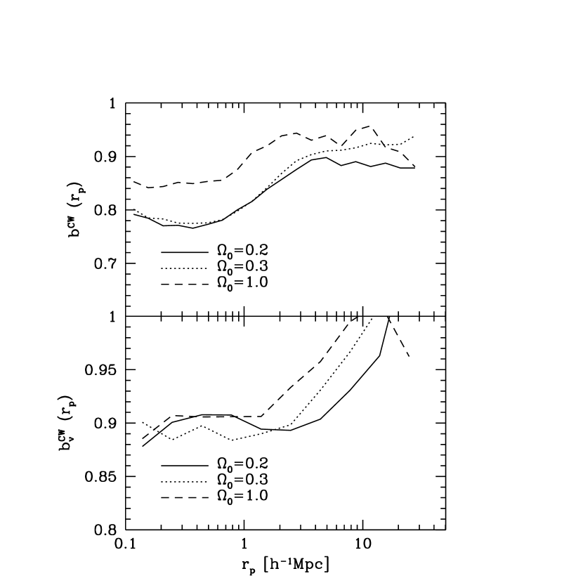
Figure 5: The biases predicted by the bias model on the projected TPCF (upper panel) and the PVD (lower panel) for the three cosmological models.

Figure 5 explicitly shows the spatial bias factor $b^{\rm CW}(r_{p})$ and the velocity bias factor $b^{\rm CW}_{v}(r_{p})$ given by our simple (Cluster-Weighting) bias scheme for the three cosmogonies. Following convention, we define $b^{\rm CW}(r_{p})$ and $b^{\rm CW}_{v}(r_{p})$ as $\sqrt{w^{\rm CW}(r_{p})/w(r_{p})}$ and $\sigma_{12}^{\rm CW}(r_{p})/\sigma_{12}(r_{p})$ respectively, where the superscript ‘CW’ labels quantities incorporating the Cluster-Weighting bias scheme. As expected, both the spatial and the velocity bias factors resulted from our bias scheme are scale-dependent, with stronger (anti)biases on smaller scales.

Having shown that our simple phenomenological bias model may be able to explain the discrepancy between the model predictions and observational results for the TPCF and PVD, we now ask whether such a bias is theoretically and observationally plausible. The bias proposed here is in the opposite sense to that proposed for the standard CDM model (e.g. White et al. 1987), because it means that the number of galaxies formed per unit mass is suppressed rather than enhanced in high density regions. One possibility for this to happen is that galaxies are systematically more massive, and so the number of galaxies per unit mass is lower (although the light per unit mass might be higher), in rich clusters than in poor clusters and groups. It is well known that rich clusters usually contain big galaxies like cDs. These galaxies are about 10 times more massive than normal $L^{*}$ galaxies, and so their share in the mass of clusters is under-represented by their number. However, cD type of galaxies are rare, and it is not clear whether the luminosity functions are significantly different between cluster and field galaxies. Another possibility is that galaxies in clusters have systematically higher mass-to-light ratios than field galaxies. In the standard picture of galaxy formation, galaxies in clusters form earlier than those in the field. Because of their old age, these galaxies might appear fainter in the observational bands and so may be under-represented in a magnitude-limited sample. Such a phenomenon has indeed been found observationally (Carlberg et al. 1997b) and in some hydro/N-body simulations (e.g. Jenkins et al. 1996).

The bias model invoked here is also consistent with current observations. Based on their detailed photometric and spectroscopic observations of rich clusters in the CNOC survey, Carlberg et al. (1996) found that the number of galaxies [brighter than $M_{r}^{K}=-18.5$ mag] per unit mass is systematically lower in clusters with higher velocity dispersions. The data show that the number of galaxies per unit mass in clusters with velocity dispersions $\lower 2.15277pt\hbox{$\;\buildrel>\over{\sim}\;$}1000\,{\rm{km\,s^{-1}}}$ is lower by a factor of about 1.5 than in poorer clusters. The implied level of bias is thus compatible with what is assumed in our bias model. At the moment the observational data are still sparse and the observed trend is not very significant. More observational data are needed to test the model we are proposing here.

It is important to emphasize that our model requires only that the number of galaxies (brighter than $-18$ mag) per unit mass decreases with cluster mass. This does not necessarily mean that the mass-to-light ratio of clusters increases with cluster mass by a proportional amount, unless the shape of the luminosity function of cluster galaxies is completely independent of cluster mass. In fact, the observational data of the CNOC clusters, which indicate a decrease of the number of galaxies per unit mass with the cluster mass, do not show any evidence for an increase of the mass-to-light ratio with cluster mass (Carlberg et al. 1996). This may already indicate that the shape of luminosity function does depend on cluster mass to some degree. Since the cosmic density parameter ($\Omega_{0}$) derived from cluster virial masses is based on the mass-to-light ratio, instead of the mass-to-number ratio, of clusters, our bias model does not necessarily imply a lower $\Omega_{0}$ value than that derived by Carlberg et al.

5 DISCUSSION

In this paper we have presented detailed comparisons with the observational results only for three spatially-flat CDM models. Some of the results may, however, apply to other interesting models of structure formation. For open CDM models with $\Omega=0.2$-0.3, $\sigma_{8}\sim 1$ and $\Gamma\sim 0.2$, the two-point mass correlation functions are slightly steeper than those for flat models with similar model parameters (see e.g. Mo, Jing & Börner 1997; Jenkins et al. 1996; Colin, Carlberg & Couchman 1996). The PVD of mass on small scales is also slightly higher (e.g. Mo, Jing & Börner 1997; Colin, Carlberg & Couchman 1996). Thus, the results for low-$\Omega$ open models are qualitatively the same as those for the low-$\Omega$ flat models considered in this paper, except perhaps that for them a higher value of $\alpha$ is needed to match the observational results. Another interesting case is the mixed dark matter (MDM) models in which 20-30 percent of the cosmic mass is in massive neutrinos (e.g. Jing et al. 1993; Klypin et al. 1993; Jing et al. 1994; Ma & Bertschinger 1995; Ma 1996). The clustering properties of dark matter predicted by such models are similar to those given by the CDM model with $\Omega_{0}=1$ and $\Gamma=0.2$. For this class of models, the predicted TPCF for the mass is quite flat and is consistent with that derived from the angular correlation function of galaxies in the APM survey (Jing et al. 1994; Jenkins et al. 1996). Thus, the kind of bias we propose here may not be needed for such models to match the observed TPCF. The PVDs of mass predicted by these models are generally lower than those predicted by the standard CDM models with the same $\sigma_{8}$ (Jing et al. 1994), because of their smaller clustering power on small scales. We thus expect that such models with $\sigma_{8}\Omega_{0}^{0.6}\sim 0.5$ are consistent with the observational result on PVD.

Based on X-ray emissions and galaxy kinematics in clusters of galaxies, Bahcall & Lubin (1994) and Carlberg et al. (1997a) found little evidence for a large velocity bias in clusters of galaxies. The velocity bias found in (some) N-body/hydro simulations of galaxy formation is also modest, with $\sigma_{\rm gal}/\sigma_{\rm DM}\sim 0.7$-0.9 (e.g. Katz et al. 1992; Cen & Ostriker 1992; Frenk et al. 1996). The finite sizes of galaxies may reduce the peculiar velocity of galaxies up to 10 percent (Suto & Jing 1997). These results imply that a large velocity bias between galaxies and mass is not supported by current observations or simulations. Unfortunately, these results are still uncertain. As we have shown, the PVD predicted by CDM models with $\sigma_{8}\Omega_{0}^{0.6}\sim 0.4$-$0.5$ is compatible with the observational result even in the absence of any velocity bias. Thus these models are consistent with current observations. For models with larger $\sigma_{8}\Omega_{0}^{0.6}$, a velocity bias is needed to make models compatible with the observed PVD. Clearly, with a better understanding of the velocity bias, our result on PVD can be used to put a stringent constraint on $\sigma_{8}\Omega_{0}^{0.6}$ in CDM models.

We have shown, with the help of large N-body simulations, that the real-space two-point correlation function and pairwise velocity dispersion of galaxies can now both be measured reliably from the LCRS. We have carried out a detailed comparison between these observational results and the predictions of current CDM cosmogonies. We have found that the observed two-point correlation function is significantly flatter on small scales than the mass correlation function predicted by current CDM models with $\sigma_{8}\Omega_{0}^{0.6}\sim 0.5$. The observed pairwise velocity dispersion is also lower than that of dark matter particles in these models. We have proposed a simple bias model to explain these discrepancies. This model assumes that the number of galaxies per unit dark matter mass, $N/M$, decreases with the mass of dark haloes increasing. The predictions of CDM models with $\sigma_{8}\Omega_{0}^{0.6}\sim 0.4$-0.5 and $\Gamma\sim 0.2$ are in agreement with the observational results, if the trend of $N/M$ with $M$ is at the level observed for rich clusters of galaxies. A velocity bias is needed for models with larger $\sigma_{8}\Omega_{0}^{0.6}$. Therefore current CDM models with $\Omega_{0}h\sim 0.2$ and with cluster-abundance normalizations are consistent with the observed correlation function and pairwise velocity dispersion of galaxies. A high level of velocity bias is not required in these models. The observational data can put a stringent constraint on the value of $\sigma_{8}\Omega_{0}^{0.6}$ in CDM models once the level of velocity bias is known.

Appendix A Testing the statistical methods

In this appendix we test whether the statistical methods described in Section 3.1 can yield unbiased measurements of the TPCF and the PVD from a sample like the LCRS. Here we generate 20 mock catalogs from one simulation of the $\Omega_{0}=0.2$ model, without including the fiber collision effect. Fiber collisions will cause some bias in the statistics, as will be discussed in Appendix B.

The projected TPCF measured directly from the mock samples is plotted as the solid circles in Figure 6, with the error bars representing the standard deviation of the mean. The thick solid curve shows $w(r_{p})$ given by the real-space two-point correlation function $\xi(r)$:

$$w(r_{p})=\int_{0}^{\infty}\xi(\sqrt{r_{p}^{2}+\pi^{2}})d\pi,$$ (A1)

where we have used the empirical model as described in Mo, Jing & Börner (1997; see also Peacock & Dodds 1996) to calculate the model prediction for $\xi$. This $w(r_{p})$ is what we want to recover from the mock samples. As shown in the figure, the result derived from the mock samples agrees well with that given by the empirical model. (The slightly higher value given by the mock samples on scales larger than $10\,h^{-1}{\rm{Mpc}}$ is due to the fact that the particular realization of the simulation used happens to have systematically higher large-scale power than average). Thus, the statistical method we have used can give an unbiased estimate of the projected TPCF. The good agreement between the mock $w(r_{p})$ and that given by the empirical formula at the small scales ($r_{p}\approx 0.1\,h^{-1}{\rm{Mpc}}$) indicates that the simulations used have sufficient resolution for the purpose of this paper.

The measurement of the PVD from mock samples based on the redshift distortion of the TPCF (as described in Section 3.1) is compared in Figure 7 to the true PVD which we want to measure. The true PVD is defined as $\langle\left\{[{\bf v}_{12}({r})-\langle{\bf v}_{12}({r})\rangle]/3\right\}^{2}\rangle^{1/2}$ where ${\bf v}_{12}({r})$ is the 3-D relative velocity of two particles with separation $r$ and $\langle\cdot\cdot\cdot\rangle$ denotes average over all pairs at separation $r$. The true PVD can be estimated from the three-dimensional velocities of particles in the simulation. Two infall models, the self-similar solution (equation 9) and the infall pattern obtained directly from the simulation, are used for reconstructing the PVD from the mock samples. The two models give very similar results on scales $r_{p}<10\,h^{-1}{\rm{Mpc}}$. Comparing the PVD reconstructed from the redshift distortion with the true value, we see that the two agree with each other qualitatively. However, the difference between the two quantities is quite significant even if the real infall pattern is used. This difference arises from the fact that the distribution of the pairwise velocities is not perfectly exponential and that the true PVD depends significantly on the separations of pairs in real space. Thus, to make a rigorous comparison between models and observational results, these systematics must be treated very carefully.

Appendix B Quantifying the effect of fiber collision

In this Appendix, we apply the same test as in Appendix A to mock samples which include the fiber collision effect. The purpose of this is to quantify the effect of fiber collisions on the two statistics presented in this paper. Figure 8 shows the ratio of $w(r_{p})$ measured from the 20 mock samples with and without fiber collisions. As expected, the effect of the fiber collisions is larger on smaller scales. The value of $w(r_{p})$ is reduced by up to 15% on the smallest scale, $r_{p}\sim 0.1\,h^{-1}{\rm{Mpc}}$. On scales $r_{p}\lower 2.15277pt\hbox{$\;\buildrel>\over{\sim}\;$}2\,h^{-1}{\rm{Mpc}}$, the effect is very small. The scatter of the ratio among different mock samples is very small, which means that the fiber collision effect is systematic and can be corrected easily in the analysis. The thin line in Fig.6 shows $w(r_{p})$ measured from the 20 mock samples with fiber collisions included.

The effect of the fiber collisions on the determination of PVD is shown in Fig.9. Here we plot the difference in $\sigma_{12}(r_{p})$ estimated by comparing 20 mock samples in which fiber collisions are included with 20 others where fiber collisions are excluded. Fiber collisions reduce the value of $\sigma_{12}(r_{p})$ by about $20\,{\rm{km\,s^{-1}}}$ for $r_{p}\lower 2.15277pt\hbox{$\;\buildrel<\over{\sim}\;$}3\,h^{-1}{\rm{Mpc}}$ and by a smaller amount for larger $r_{p}$. This result depends very weakly on the infall model adopted.

We have tested the robustness of the above results to the change in the intrinsic clustering, applying the same tests to the cluster weighted mock samples (section 3.2) of the $\Omega_{0}=0.2$ model. The statistical results are the same as those presented in Figures 8 and 9. Thus the effects of fiber collisions on TPCF and PVD are not sensitive to the intrinsic clustering, and the results presented in this Appendix can be used to correct for the fiber collision effects in the LCRS.

Figure 1: The projected two-point correlation function measured from the Las Campanas Redshift Survey (filled triangles). Error bars are $1\sigma$ deviations given by bootstrap resampling. Results for the north and south subsamples are shown by the dotted and dashed lines, respectively. The solid line is the power-law fit to the correlation function of the total sample.

Figure 2: The pairwise velocity dispersion $\sigma_{12}(r_{p})$ measured from the Las Campanas Redshift Survey (filled triangles). Error bars are $1\sigma$ deviations given by bootstrap resampling. Results for the north and south subsamples are shown by the dotted and dashed lines, respectively.

Figure 3: Comparison of the predictions of CDM models with the LCRS results. Left panels– the projected two-point correlation function. Triangles show the observational result from Fig. 1. The mean value and the $1\sigma$ limits predicted by the CDM models are shown by the thick and thin lines respectively. The dashed lines in the lowest panel are obtained by shifting the solid lines upwards by an amount of $1/\sigma_{8}^{2}$. Right panels– the pairwise velocity dispersion. Thick and thin lines show the mean value and the 1$\sigma$ limits predicted by the CDM models. The solid lines show the results obtained from the self-similar infall model, while the dashed lines are those obtained from the real infall pattern given by simulations of the model under consideration. Triangles show the result for the LCRS obtained from the self-similar infall model; circles show the result when the infall pattern given by the simulations is used. Error bars for the LCRS results are shown only for the self-similar infall model.

Figure 4: The predictions of the three CDM models incorporating a simple bias model (see text). The lines and symbols have the same meaning as in Fig.3. The dashed lines in the lower-left panel are obtained by shifting the solid lines upwards by an amount, $1/\sigma_{8}^{2}$.

Figure 6: The projected two-point correlation function for the $\Omega_{0}=0.2$ model estimated from 20 mock samples without fiber collisions (filled circles). Error bars are the ($1\sigma$) standard deviations of the mean from the mock samples. The thick solid line is the model prediction based on the empirical fitting formula. The thin line shows the result for the 20 mock samples including the fiber-collision effect.

Figure 7: The pairwise velocity dispersion $\sigma_{12}(r_{p})$ measured from the redshift distortion of the two-point correlation function of the 20 mock samples without fiber collisions. Two infall models are adopted for $\overline{v_{12}}(r)$: the self-similar infall model (triangles) and the infall pattern derived directly from the simulations (circles). The true pairwise velocity dispersion given by the 3-dimensional velocities in the simulations is shown as the solid line. Error bars are the ($1\sigma$) standard deviations of the mean from the mock samples.

Figure 8: The ratio of the projected two-point correlation functions measured from 20 mock samples with and without fiber collisions. Error bars are the ($1\sigma$) standard deviation of the mean from the mock samples.

Figure 9: The difference between the pairwise velocity dispersions estimated for 20 mock samples with and without fiber collisions. Results are shown for the two infall models, as in Fig.6. Error bars are the ($1\sigma$) standard deviation of the mean from the mock samples.

References

- (1)
- (2) Bahcall N.A., Fan X.H., Cen R., 1997, preprint (astro-ph/9706018)
- (3)
- (4) Bahcall N.A., Lubin L.M., 1994, ApJ, 426, 513
- (5)
- (6) Bardeen J., Bond J.R., Kaiser N., Szalay A.S., 1986, ApJ, 304, 15
- (7)
- (8) Barrow J.D., Bhavsar S.P., Sonoda D.H., 1984, MNRAS, 210, 19
- (9)
- (10) Baugh C.M., 1996, MNRAS, 280, 267
- (11)
- (12) Bean A.J., Efstathiou G., Ellis R.S., Peterson B.A., Shanks T., 1983, MNRAS, 205, 605
- (13)
- (14) Carlberg R.,G., Couchman H.M.P., 1989, ApJ, 340, 47
- (15)
- (16) Carlberg R.,G., Yee H.,K.,C., Ellingson E., Abraham R., Gravel P., Morris S., Pritchet C.J., 1996, ApJ, 462, 32
- (17)
- (18) Carlberg R.G., et al., 1997a, preprint (astro-ph/9703107)
- (19)
- (20) Carlberg R.G., et al., 1997b, preprint (astro-ph/9704060)
- (21)
- (22) Cen R.Y., Ostriker J., 1992, ApJ, 399, L113
- (23)
- (24) Colin P., Carlberg R.G., Couchman H.M.P., 1996, preprint (astro-ph/9604071)
- (25)
- (26) Davis M., Peebles P.J.E., 1983, ApJ, 267, 465
- (27)
- (28) Dekel A., Rees M.J., 1987, Nat, 326, 455
- (29)
- (30) Diaferio A., Geller M.J., 1996, ApJ, 467, 19
- (31)
- (32) Eke V., Cole S., Frenk C.S., 1996, MNRAS, 282, 263
- (33)
- (34) Efstathiou G., Sutherland W.J., Maddox S.J., 1990, Nat, 348, 705
- (35)
- (36) Fisher K.B., Davis M., Strauss M.A., Yahil A., Huchra J.P., 1994, MNRAS, 267, 927
- (37)
- (38) Frenk C.S., Evrard A.F., White S.D.M., Summers F.J., 1996, ApJ, 472, 460
- (39)
- (40) Guzzo L., Fisher K.B., Strauss M.A., Giovanelli R., Haynes M.P., 1995, preprint
- (41)
- (42) Hamilton A.J.S., 1993, ApJ, 417, 19
- (43)
- (44) Jenkins A., et al., 1996, preprint (astro-ph/9610206)
- (45)
- (46) Jing Y.P., Fang L.Z., 1994, ApJ, 432, 438
- (47)
- (48) Jing Y.P., Mo H.J., Börner G., Fang L.Z., 1993, ApJ, 411, 450
- (49)
- (50) Jing Y.P., Mo H.J., Börner G., Fang L.Z., 1994, A&A, 284, 703
- (51)
- (52) Katz, N., Hernquist, L., Weinberg, D.H. 1992, ApJ, 399, L109
- (53)
- (54) Kitayama, T., Suto, Y. 1997, Preprint (astro-ph/9702017)
- (55)
- (56) Klypin A., Holtzman J., Primack J., Regos E., 1993, ApJ, 416, 1
- (57)
- (58) Klypin A., Primack J. Holtzman J. 1996, ApJ, 466, 13
- (59)
- (60) Lin H., Kirchner R.P., Shectman S.A., Landy S.D., Oemler A.,Tucker D.L Schechter P.L., 1996, ApJ, 464, 60
- (61)
- (62) Lin H. et al. 1997, in preparation
- (63)
- (64) Ma, C.-P. 1996, ApJ, 471
- (65)
- (66) Ma, C.-P., Bertschinger, E. 1994, ApJ, 429, 22
- (67)
- (68) Maddox S.J. Efstathiou G., Sutherland W.J., Loveday, J. 1990, MNRAS, 242, p43
- (69)
- (70) Maddox S.J. Efstathiou G., Sutherland W.J., 1996, MNRAS, 283, 1227
- (71)
- (72) Marzke R.O., Geller M.J., daCosta L.N., Huchra J.P., 1995, AJ, 110, 477
- (73)
- (74) Mo H.J., Jing Y.P., Börner G., 1992, ApJ, 392, 452
- (75)
- (76) Mo H.J., Jing Y.P., Börner G., 1993, MNRAS, 264, 825
- (77)
- (78) Mo H.J., Jing Y.P., Börner G., 1997, MNRAS, 286, 979
- (79)
- (80) Peacock J.A., 1997, MNRAS, 284, 885
- (81)
- (82) Peacock J.A., Dodds S.J., 1996, MNRAS, 280, L19
- (83)
- (84) Peebles P.J.E., 1980, The Large-Scale Structure of the Universe, Princeton University Press, Princeton
- (85)
- (86) Ratcliffe A., Shanks T., Fong R., Parker Q.A., 1997, preprint (astro-ph/9702228)
- (87)
- (88) Shectman S. A., Landy, S.D., Oemler A., Tucker D.L., Lin H., Kirshner R.P., Schechter P.L., 1996, ApJ, 470, 172
- (89)
- (90) Sheth R., 1996, MNRAS, 279, 1310
- (91)
- (92) Somerville R., Davis M., Primack J.R., 1997, ApJ, 479, 616
- (93)
- (94) Suto Y., 1993, Prog. Theor. Phys., 90, 1173
- (95)
- (96) Suto Y., Jing Y.P. 1997, ApJS, 110, 167
- (97)
- (98) Viana P.T.P., Liddle A.R., 1996, MNRAS, 281, 323
- (99)
- (100) White S.D.M., Efstathiou G., Frenk C., 1993, MNRAS, 262, 1023
- (101)
- (102) White S.D.M., Davis M., Efstathiou G., Frenk C., 1987, Nat, 330, 451
- (103)
- (104) Zurek W., Quinn P.J., Salmon T.K., Warren M.S., 1994, ApJ, 431, 559
- (105)