Holes in the Microwave Sky

Abstract

We discuss the implications of two possible, recent Sunyaev-Zel’dovich (SZ) detections for which no optical or X–ray counterparts have been found. This suggests that the objects reside at high redshift, which is difficult to reconcile with a critical cosmology. We develop this argument and find that an open model with $\Omega_{\rm o}=0.2$ remains consistent with what we currently know about the two objects. The reasoning also demonstrates the utility of SZ cluster searches.

Observatoire de Strasbourg, 11, rue de l’Université
67000 Strasbourg, FRANCE

Danish Space Research Institute, DSKI Juliane Maries Vej 30
DK-2700, Copenhagen 0, DENMARK

1 Introduction

By holes in the microwave sky, we hope to invoke an image of the Sunyaev–Zel’dovich (SZ) effect at low frequences: a region of lower than average sky brightness, or a hole in the cosmic microwave background (CMB). The image presented by B. Partridge at these proceedings is an excellent example and, along with a similar detection by the Ryle Telescope, is the motivation for this presentation; because if the two radio decrements are indeed due to SZ effect, this can have powerful implications for the value of $\Omega_{\rm o}$.

In what has yielded the deepest radio map to date, the VLA discovered a radio decrement – characteristic of the SZ effect below 1.4 mm – during an observation of one of the HST Medium Deep Survey fields (Richards et al. [1996]). The object is just resolved, extending over an area of about $30\times 60\;{\rm arcsec}^{2}$. The other object (Jones et al. [1996]) was found by the RYLE Telescope (RT) during an ongoing program of double quasar observations (Saunders [1997]). They find a radio decrement covering an area of about $120\times 180\;{\rm arcsecs}^{2}$. In both cases, subsequent follow–up in the optical and in the X–ray band has not reveiled the supposed clusters (Richards et al. [1996]; Jones et al [1996]; Saunders et al. [1997]). Definite confirmation of the SZ nature of the two decrements will thus come from efforts to measure the effect at different frequencies, to see if the spectra are consistent with the SZ effect. If they are indeed clusters, then the lack of optical or X–ray counterparts may be interpretated as evidence that they lie at large redshift. It is in this way that we may obtain very strong constraints on $\Omega_{\rm o}$: The number of massive, high–redshift clusters depends sensitively on $\Omega_{\rm o}$, so much so that the observation of even a small number of such clusters can eliminate the critical model (Oukbir & Blanchard [1992]; Barbosa et al. [1996]; Eke et al. [1996]; Oukbir & Blanchard [1997]).

2 The Mass Function and $\Omega_{\rm o}$

The easiest way to understand this dependence is by considering the mass function, the number density of collapsed objects as a function of mass and redshift (e.g., Bartlett [1997]). In ‘standard’ models, based on the growth of initially small density perturbations with gaussian statistics, this takes the general form of a power law times a gaussian (Press & Schechter [1974]):

$$\frac{dn}{d{\rm ln}M}=\sqrt{\frac{2}{\pi}}\frac{<\rho>}{M}\nu(M,z)\left(-\frac{d{\rm ln}\sigma(M,z)}{d{\rm ln}M}\right)e^{-\nu^{2}/2}.$$ (1)

In this equation, $<\rho>$ is the mean, comoving density of the Universe and $\sigma(M,z)$ is the power spectrum as a function of the mass scale, $M$. The quantity

$$\nu(M,z)=\frac{\delta_{c}(z)}{\sigma_{\rm o}(M)}\frac{D_{\rm g}(z=0)}{D_{\rm g}(z)}$$ (2)

is a function of the linear growth factor, $D_{\rm g}(z;\Omega_{\rm o},\Lambda)$, which depends on $\Omega_{\rm o}$ and $\Lambda$, of the critical density needed for collapse, $\delta_{c}$, which has only a weak dependence on $\Omega_{\rm o}$ and $\Lambda$, and of $\sigma_{\rm o}(M)$, the present–day power spectrum, a function of mass only. The appearance of $D_{\rm g}$ in the exponential of the mass function indicates that the $\Omega_{\rm o}$ dependence can be quite strong; hence, the comment that even a small number of clusters at large $z$ can severely constrain the density parameter. The key point is that the shape of the redshift distribution of clusters of a given mass is only determined by the cosmological parameters (the power spectrum cannot be changed to alter this fact) (Oukbir & Blanchard [1997]).

The problem is that we do not measure mass directly; we need some other, more readily observable quantity which correlates well with cluster mass. Because we believe that the hot cluster gas is heated by infall during cluster formation, we expect that the X–ray temperature should represent the depth of the cluster potential well and, therefore, its mass. This has in fact been well established by various hydrodynamical simulations (in ‘standard’ scenarios) (Evrard et al. [1996]), which also provide the exact form of the temperature–mass relation. The X–ray luminosity, on the other hand, is a more complicated animal, depending not only on the temperature of the gas, but also on its abundance and spatial distribution. As we discuss below, observing clusters via the Sunyaev–Zel’dovich effect avoids these problems associated with the X–ray flux, while preserving the simplicity of a straightforward flux measurement (plus other advantages). This is important because X–ray spectra demand time–consuming, space–based observations.

Table
Model Parameters - normalized to the local X–ray temperature function^a

$\Omega_{\rm o}$	$h$	$\sigma_{8}$	$n$
0.2	0.5	1.37	-1.10
1.0	0.5	0.61	-1.85

$a$ - Henry & Arnaud ([1991])

For our discussion here, we take a phenomenological point–of–view and adopt a power–law approximation to the power spectrum: $\sigma_{\rm o}=(1/b)(M/M_{8})^{-\alpha}$, where $b$ is the bias parameter and $M_{8}$ is the mass contained in a sphere of $8\;h^{-1}\;{\rm Mpc}$. We will focus on the comparison of two extreme models, a critical model and an open model with $\Omega=0.2$ ($h=H_{o}/100\;{\rm km/s/Mpc}=1/2$ in both cases). The parameters $b$ and $\alpha$ for each model are constrained by fitting to the local X–ray temperature function of galaxy clusters (Henry & Arnaud [1991]), the results of which are given in the Table (Oukbir et al. [1997]; Oukbir & Blanchard [1997]).

3 The Sunyaev-Zel’dovich Effect

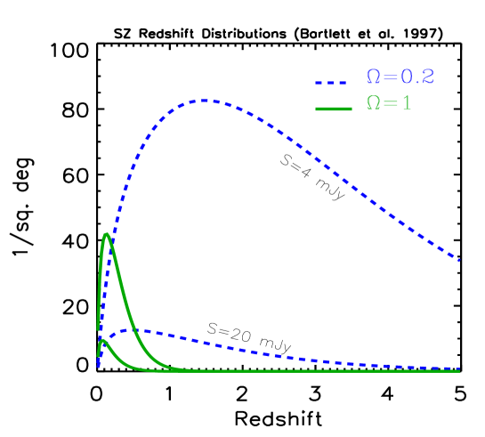
Figure 1: Redshift distribution for clusters of given SZ flux density in the two cosmological models – critical (solid lines) and open with $\Omega=0.2$ (dashed lines); see the Table for the model parameters. The curves are drawn for $S_{sz}=4\;{\rm mJy}$ and $S_{sz}=20\;{\rm mJy}$, corresponding to the VLA and RT objects, respectively, when translated to $\lambda=0.75\;{\rm mm}$. For clarity, the two curves for the critical model are not labeled explicitly. We adopt $h=1/2$.

The Sunyaev-Zel’dovich effect offers unique advantages for finding high redshift clusters and quantifying their abundance. The surface brightness of a cluster relative to the unperturbed CMB is expressed as a product of a spectral function, $j_{\nu}$, and the Compton $y$–parameter, which is an integral of the electron pressure along the line–of–sight: $y\propto\int dl\;n_{e}T$. Integrating the surface brightness over solid angle yields the following functional form for the total flux density of a cluster with angular size $\theta$:

$$S_{sz}\propto\theta^{2}n_{e}Tl\propto M_{gas}TD_{a}^{-2}(z)$$

$$\propto f_{gas}M_{tot}^{5/3}(1+z)D_{a}^{-2}(z),$$ (3)

where $M_{tot}$ is the total, virial mass of the cluster, $f_{gas}$ is the hot gas mass fraction of clusters and $D_{a}(z)$ is the angular–size distance. In the last line, we have used the fact that there exists a tight relation between X–ray temperature and virial mass: $T\propto M^{2/3}(1+z)$ (Evrard et al. 1996). Let’s compare this with the corresponding expression for the X–ray flux of a cluster:

$$f_{x}=\theta^{2}n_{e}^{2}T^{1/2}l(1+z)^{-4}\propto n_{e}M_{gas}T^{1/2}D_{a}^{-2}(z)(1+z)^{-4}$$

$$\propto n_{e}f_{gas}M_{tot}T^{1/2}D_{l}^{-2}(z),$$ (4)

with $D_{l}$ denoting the luminosity distance. By comparing these two expressions we see that, in contrast to the SZ flux density, the X–ray flux suffers cosmological surface brightness dimming, represented by the extra factors of $(1+z)$ in the denominator of Eq. (3) which convert the angular–size distance to the luminosity distance. Besides this well–known difference, which tells us that the SZ effect is the more efficient way to find high–redshift clusters, we note that the X–ray emission depends on the gas density in addition to the hot gas mass fraction and temperature. This is unfortunate, because it means that the X–ray flux from a cluster depends on the core radius and profile of the intracluster medium (ICM) – two quantities which are poorly, if at all, understood from the theoretical point of view. The SZ flux density presents the important advantage that it depends only on the total gas mass and the temperature, and not on the ICM’s distribution. It is also true that the temperature which appears in the expression for the SZ flux density is a simpler quantity than the X–ray measured temperature: it is the mean, particle–weighted energy of the gas particles instead of, as in the case of X–rays, the emission–weighted gas temperature. This SZ temperature is a quantity which should be all the more closely related to the virial mass of a cluster than even the X–ray temperature, and less affected by any temperature structure in the cluster.

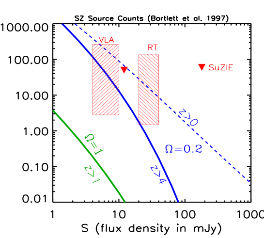
Figure 2: SZ source counts with observational constraints, as a function of SZ flux density expressed at $\lambda=0.75\;{\rm mm}$. The two hatched boxes show the 95% one–sided confidence limits from the VLA and the RT; due to the uncertain redshift of the clusters, there is a range of possible total SZ flux density, which has for a minimum the value observed in each beam and a maximum chosen here to correspond to $z>1$. From the SuZIE blank fields, one can deduce the 95% upper limit shown as the triangle pointing downwards (Church et al. [1997]). We also plot the predictions of our fiducial open model ($\Omega=0.2$) for all clusters (dashed line) and for those clusters with $z>4$. The critical model has great difficulty explaining the observed objects even with a lower redshift cutoff of only $z>1$; the actual limit from the X–ray data is stronger, but this would fall well off to the lower left of the plot. We assume $h=1/2$.

Now the game is clear: with Eq. (3) we may convert the mass function into a distribution of clusters in SZ flux density and redshift (the quantitative relation for $S_{sz}$ can be found in Barbosa et al. [1996]). The redshift distribution of clusters and the total source counts are then easily calculable (Korolyov et al. [1986]; Markevitch et al. [1994]; Bartlett & Silk [1994]; Barbosa et al. [1996]; Eke et al. [1996]; Colafrancesco et al. [1997]). In Figure 1, we show the redshift distribution for clusters of two given SZ flux densities and for two representative cosmologies – a critical model and a model with $\Omega=0.2$ and $\Lambda=0$. For this calculation, we have used a constant gas mass fraction $f_{gas}=0.06\;h^{-3/2}\;$ (Evrard [1997]). The two chosen fluxes are our estimates of the flux density of the VLA and RT objects, when translated to a wavelength of $\lambda=0.75\;{\rm mm}$ by using the SZ spectral function, $j_{\nu}$; this is our fiducial working frequency and corresponds to the peak of the SZ distortion.

The key aspect of this figure is that, at a given flux density, there is an enormous difference between the number of high–redshift clusters in a critical and open universe. It is for this reason that even the detection of only two SZ decrements warrants the present discussion, because they appear to be at large redshift. Let us now quantify this by comparing the predicted number counts of clusters with redshifts greater than some minimum value with the counts implied by the detection of these two objects. This is done in Figure 2. The observed counts have been estimated using Poisson statistics and the amount of sky coverage in each case – $\sim 0.018\;{\rm deg}^{2}$ for the VLA (two fields) and $\sim 0.034\;{\rm deg}^{2}$ for the RT (three fields). These constraints are given as two boxes because there is actually a range of possible total SZ flux density from each object, due to the unknown redshifts: at low redshift, the objects would be resolved and their flux density has to be corrected upwards. The minimum flux density is clearly the value observed, while for the maximum, we give the values for $z\sim 1$ assuming an isothermal $\beta-{\rm model}$. The limits on the counts (i.e., in the vertical direction) are generous in that they represent the 95% one–sided Poisson confidence limits. We also show an upper limit on the counts obtained by the SuZIE instrument (Church et al. [1997]), which found no objects in a survey area of $\sim 0.06\;{\rm deg}^{2}$ down to the limiting flux shown; the symbol represents the resulting 95% confidence upper limit. Predictions for the number of clusters on the sky for the two cosmological models and with varying minimum redshifts are shown by the labeled curves.

4 Conclusions

The basic result from Figure 2 is clear: if the two radio decrements are indeed due to the thermal SZ effect in two clusters, then the critical model is in very serious trouble. On the other hand, an open model is capable of explaining the objects. While our modeling has been rather simple in that we have used power–law power spectra and assumed that the cluster gas fraction is constant over mass and epoch (see, e.g., Colafrancesco et al. [1997] for more detailed treatment of cluster evolution), in the present circumstance any reasonable evolution in the gas mass fraction would lead to a decrease in the SZ flux density of objects with small mass and/or at large redshift; hence, it would only make things more difficult for the critical model.

What about other possible caveats? Besides the fact that we still await definite confirmation of the true nature of the radio decrements (e.g., detections at other frequencies), the most important thing to be wary of is the possible bias associated with the fact that the RT was pointed at a known double quasar, not an a priori blank field. This seems less likely to be true of the VLA detection, in as much as there was no previously known quasar pair in that field (although one was subsequently found). In any case, we should have a better idea in the near future from other experiments as the amount of sky covered by SZ searches appears to be rapidly increasing. The present discussion brings to light the importance of such SZ searches (we note in particular that a $\sim 1$ square–degree search with the BIMA telescope is now feasible [Holzapfel, private communication]). A satellite mission covering the full sky, such as the Planck Surveyor, will be the culmination of such efforts.

Finally, we remark that the possible existence of clusters at redshifts much greater than unity should not be seen as exotic; quite the contrary, in open models, they are expected. If they are indeed out there, they would not have been detectable up until now by either optical or X–ray observations. One would imagine that they would first be seen by SZ searches, and these are just now beginning to provide some very interesting and tantalizing hints.

References

- 1996 Barbosa D., Bartlett J.G., Blanchard A. & Oukbir J. 1996, A&A, 314, 13.
- 1997 Bartlett J.G. 1997, in: From Quantum Fluctuations to Cosmological Structures, School held in Casablanca, in press astro-ph/9703090.
- 1994 Bartlett J.G. & Silk J. 1994, ApJ 423, 12.
- 1997 Church S.E., Ganga K.M., Ade P.A.R., Holzapfel W.L., Mauskopf P.D., Wilbanks T.M. & Lange A.E. 1997, ApJ, 484, 523.
- 1997 Colafrancesco S., Mazzotta P., Rephaeli Y. & Vittorio N. 1997, ApJ 479, 1.
- 1996 Eke V.R., Cole S. & Frenk C.S. 1996, MNRAS 282, 263.
- 1997 Evrard A.E. 1997, astro-ph/9701148.
- 1996 Evrard A.E., Metzler C.A. & Navarro J.F. 1996, ApJ, 469, 494.
- 1991 Henry J.P. & Arnaud K.A. 1991, ApJ, 372, 410.
- 1996 Jones M.E., Saunders R., Baker J.C., Cotter G., Edge A., Grainge K., Haynes T., Lasenby A., Pooley G., Röttgering H. 1997, ApJL, 479, L1.
- 1986 Korolyov V.A., Sunyaev R.A. & Yakubtsev L.A. 1986, Sov. Astron. 12, L141.
- 1994 Markevitch M., Blumenthal G.R., Forman W., Jones C. & Sunyaev R.A. 1994, ApJ 426, 1.
- 1992 Oukbir J. & Blanchard A. 1992, A&A 262, L21.
- 1997 Oukbir J. & Blanchard A. 1997, A&A, 317, 1.
- 1997 Oukbir J., Bartlett J.G. & Blanchard A. 1997, A&A, 320, 365.
- 1974 Press W.H. & Schechter P. 1974, ApJ, 187, 425.
- 1996 Richards E.A., Fomalont E.B., Kellermann K.I., Partridge R.B., Windhorst R.A. 1996, astro-ph/9612183.
- 1997 Saunders R. 1997, in: Microwave Background Anisotropies, to appear in the proceedings of the XXXIst Rencontre de Moriond, astro-ph/ 9611213.
- 1997 Saunders R., Baker J.C., Bremer M.N., Bunker A.J., Cotter G., Eales S., Grainge K., Haynes T., Jones M.E., Lacy M., Pooley G. & Rawlings S. 1997, ApJL, 479, L5.