$H_{2}^{+}$ ion in strong magnetic field: a variational study

Abstract

Using a single trial function we perform an accurate calculation of the ground state $1\sigma_{g}$ of the hydrogenic molecular ion $H^{+}_{2}$ in a constant uniform magnetic field ranging $0-10^{13}$ G. We show that this trial function also makes it possible to study the negative parity ground state $1\sigma_{u}$. We obtain that over the whole range of magnetic fields studied, the calculated binding energies are in most cases larger than binding energies obtained previously by other authors using different methods.

I Introduction

For a long time the behavior of atomic and molecular systems in a strong magnetic field of order $B\geq 10^{9}$ G has attracted considerable attention. The main interest comes from both astrophysics – studies of white dwarfs and neutron stars (see [1, 2], and also, for example [3, 4], and the review [5] and references therein), as well as from chemistry – formation of unusual chemical compounds whose existence is impossible without strong magnetic fields [6] (for a review, see, for example, [7] and references therein).

There are many studies of the hydrogen atom $H$ – the simplest atomic system – in a strong magnetic field, while the hydrogen molecular ion $H^{+}_{2}$ – the simplest molecular system which is stable with respect to dissociation $H^{+}_{2}\rightarrow H+p$ – is much less explored. One of the major drawbacks of many of these studies is a restricted domain of applicability: they are accurate in the weak magnetic field region but are inappropriate for the strong magnetic field region and vice versa. The goal of the present Note is to carry out an accurate variational calculation of $H^{+}_{2}$ in magnetic fields ranging from 0 up to $10^{13}$ G using a unique simple trial function equally applicable for any value of the magnetic field strength. We restrict our consideration to the case where the magnetic field is directed along the axis of the molecule, which is evidently the optimal configuration leading to the lowest energy. Our main perception is that the calculations should not be technically complicated and also easily reproduced, while the trial function should be simple enough to allow further analytic and numerical investigations.

II Choice of trial functions

A constructive criterion for an adequate choice of trial function was formulated in [8] and further development was presented in [9, 10]. In the simplest form the criterion is the following. The trial function $\Psi_{t}(x)$ should contain all symmetry properties of the problem in hand. If the ground state is studied, the trial function should not vanish inside of the domain where the problem is defined. The potential $V_{t}(x)=\frac{{\mathbf{\nabla}}^{2}\Psi_{t}}{\Psi_{t}}$, for which the trial function is an eigenfunction, should reproduce the original potential near singularities and also its asymptotic behavior. The use of this simplest possible recipe has led to a unique one-parameter trial function, which, in particular made it possible to carry out the first qualitative study of the ground state of the hydrogen molecule $H_{2}$ in the region of both weak and strong magnetic fields [11]. Later a few-parameter trial function was proposed for a description of the hydrogen atom in an arbitrary magnetic field, which led, for the low-excited states, to an accuracy comparable with the best calculations [10, 12].

Now we wish to apply the above-mentioned recipe to the ion $H_{2}^{+}$. We work in the Born-Oppenheimer approximation. Let us first introduce notation (see Fig.1). We consider two attractive centers of charge $Z$ situated on the $z$-axis at a distance $R/2$ symmetrically with respect to the origin. The magnetic field of the strength $B$ is directed along the $z$ axis and $r_{1,2}$ are the distances from the electron to the first(second) center, respectively. The quantity $\rho$ is the distance from the electron to the $z$-axis. Through the paper the Rydberg is used as the energy unit. For the other quantities standard atomic units are used. The potential corresponding to the problem we study is given by

$$V\ =\ \frac{2Z^{2}}{R}-\frac{2Z}{r_{1}}-\frac{2Z}{r_{2}}+\frac{B^{2}\rho^{2}}{4}\ ,$$ (1)

where the first term has the meaning of the classical Coulomb energy of the interaction of two charged centers.

One of the simplest functions satisfying the above recipe is the Heitler-London function multiplied by the lowest Landau orbital:

$$\Psi_{1}={e}^{-\alpha_{1}Z(r_{1}+r_{2})-\beta_{1}B\rho^{2}/4},$$ (2)

where $\alpha_{1},\beta_{1}$ are variational parameters. It has in total 3 variational parameters if we include the internuclear distance $R$, in the search for the equilibrium distance. It is known that in the absence of a magnetic field a function of the Heitler-London type gives an adequate description of diatomic systems near their equilibrium position. The potential corresponding to this function is:

$$V_{1} = 2Z^{2}\alpha^{2}_{1}-B\beta_{1}-2Z\alpha_{1}\Big{(}\frac{1}{r_{1}}+\frac{1}{r_{2}}\Big{)}+\frac{\beta^{2}_{1}B^{2}\rho^{2}}{4}$$ (4)

$$+\ 2Z^{2}\frac{\alpha^{2}_{1}}{r_{1}r_{2}}\Big{[}\rho^{2}+(z-R/2)(z+R/2)\Big{]}+Z\alpha_{1}B\beta_{1}\rho^{2}\Big{(}\frac{1}{r_{1}}+\frac{1}{r_{2}}\Big{)}\ .$$

It is clear that this potential reproduces the original potential (1) near Coulomb singularities and at large distances, $|x|\rightarrow\infty$.

The Hund-Mulliken function multiplied by the lowest Landau orbital is another possible trial function:

$$\Psi_{2}=\Big{(}{e}^{-\alpha_{2}Zr_{1}}+e^{-\alpha_{2}Zr_{2}}\Big{)}{e}^{-\beta_{2}B\rho^{2}/4}\ ,$$ (5)

where $\alpha_{2},\beta_{2}$ are variational parameters. It is well known that this function, in the absence of a magnetic field, describes the region of large internuclear distances. The calculations we performed show that this property remains valid for all magnetic fields up to $10^{13}$ G. Like (2), the trial function (4) is characterized by 3 variational parameters. In order to take into account both equilibrium and large distances, we should use an interpolation of (2) and (4). There are two natural ways to interpolate:

• a non-linear superposition:

  $$\Psi_{3-{1}}=\Big{(}{e}^{-\alpha_{3}Zr_{1}-\alpha_{4}Zr_{2}}+\sigma{e}^{-\alpha_{4}Zr_{1}-\alpha_{3}Zr_{2}}\Big{)}{e}^{-\beta_{3}B\rho^{2}/4}\ ,$$ (6)

  where $\alpha_{3},\alpha_{4},\beta_{3}$ are variational parameters. The parameter $\sigma=\pm 1$ depends on whether positive parity $1\sigma_{g}$ or negative parity $1\sigma_{u}$ states we consider. The function (5) is a modification of the Guillemin-Zener function used for the description of the molecular ion $H^{+}_{2}$. If $\alpha_{3}=\alpha_{4}$, the function (5) reduces to (2) and if $\alpha_{3}=0$, it coincides with (4). In total there are 4 variational parameters characterizing the trial function (5);

• a linear superposition of (2), (4)

  $$\Psi_{3-{2}}=A_{1}\Psi_{1}+A_{2}\Psi_{2}\ ,$$ (7)

where the relative weight of (2) and (4) in (6) is taken as an extra variational parameter. It is a 7-parameter trial function.

Of course, as a natural continuation of the above interpolation procedure one can take a linear superposition of all three functions: the modified Heitler-London, Hund-Mulliken and Guillemin-Zener functions (2), (4), (5)

$$\Psi_{4}=A_{3-{1}}\Psi_{3-{1}}+A_{3-2}\Psi_{3-{2}}=A_{3-{1}}\Psi_{3-{1}}+A_{1}\Psi_{1}+A_{2}\Psi_{2}\ ,$$ (8)

where again, as in the case of the function (6) the relative weights of different components are variational parameters. In total, the trial function (7) is characterized by 10 variational parameters. Most of our calculations will be carried out using this function. The minimization procedure was done using the standard minimization package MINUIT from CERN-LIB on a Pentium-Pro PC.

III Results

In order to present our results we begin with the study of the dependence of our variational results on different trial functions (see Table 1). It turned out that all variational parameters are of the order of one independently on the value of the magnetic field strength. In the Table 2 we give a comparison of our calculations with the best known results. Since we are doing a variational study of the problem, the (binding) energies obtained represent (lower) upper bounds to the exact energies. No need to mention that many calculations were performed for the case of the $H^{+}_{2}$ ion in absence of a magnetic field. Our results are in agreement with the best calculations within an absolute accuracy of $10^{-5}$. For all studied values of the magnetic field ($\leq 10^{13}$ G) our results for binding energies exceed the best known results at the present. Among all previously made calculations, we should emphasize that those performed by Wille [14] have the most extended domain of applicability. The accuracy of these results is almost as good as the accuracy of our results for magnetic fields $B\leq 10^{11}$ G. However for bigger magnetic fields the accuracy of his results fells down drastically.

Fig.2 shows the electronic density distribution as a function of magnetic field. For a small magnetic field the distribution has two clear maxima corresponding to the positions of the centers. The situation changes drastically for magnetic fields of the order of $B\simeq 3\times 10^{11}$ G, where the probability of finding the electron in any position between the two centers is practically the same. For larger magnetic fields the electron is preferably located between the two centers with the maximum in the middle, $z=0$ (see Fig 2 (e), (f)). Due to a loss of accuracy this phenomenon was not observed in [14]. It is worth noticing that for all magnetic fields studied the region of large internuclear distances is dominated by the Hund-Mulliken function (4).

In Table 3 the results of the study of the ground state of negative parity $(1\sigma_{u})$ are presented. Let us note that in the absence of a magnetic field the electron is not bounded possessing a shallow minimum (see, for example, [13, 15]). However, in a magnetic field the electron becomes bounded in agreement with general expectations [6] (see also [15]).

In conclusion we want to emphasize that we present the most accurate calculations for the ground state energies and equilibrium distances of the molecular ion $H^{+}_{2}$ in magnetic field. Unlike the majority of other studies our calculations stem from a unique framework covering both weak and strong magnetic field regimes.

FIG. 1.: $H_{2}^{+}$ in a magnetic field $B$. Explanation of the notations used

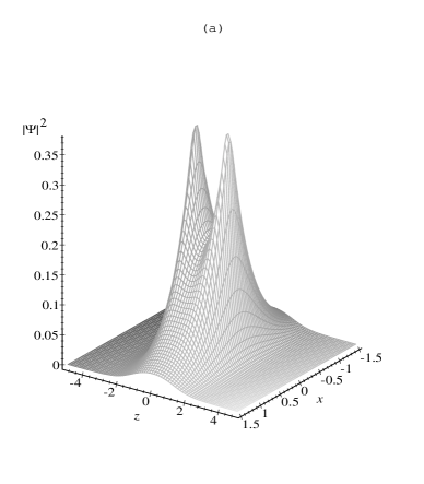
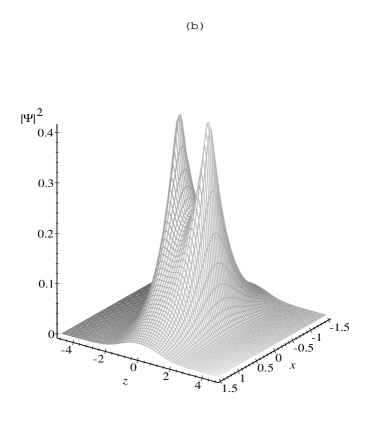
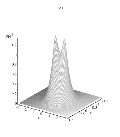
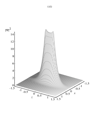
FIG. 2.: The electronic probability density of the ground state $1\sigma_{g}$ at $y=0$ as a function of the magnetic field strength. (a) $B=0$, (b) $B=10^{9}$ G, (c) $B=10^{10}$ G, (d) $B=10^{11}$ G.

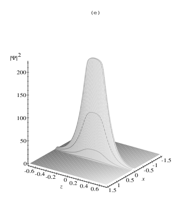
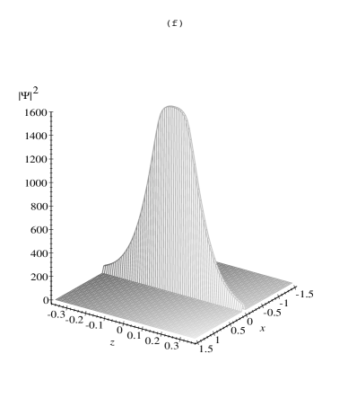
FIG. 2.: (Continuation) (e) $B=10^{12}$ G, (f) $B=10^{13}$ G.

TABLE I.: Ground state energies and the equilibrium distances for the ground state $1\sigma_{g}$ of the ion $H_{2}^{+}$ obtained using different trial wave functions as a function of the magnetic field strength.

$B$		$\Psi_{1}$	$\Psi_{2}$	$\Psi_{3-1}$	$\Psi_{3-2}$	$\Psi_{4}$
$0$	$E$	-1.16277	-1.17299	-1.20488	-1.20488	-1.20525
	$R$	1.84678	2.00349	1.99799	1.99810	1.99706
$10^{9}$ G	$E$	-1.11760	-1.11849	-1.15007	-1.15013	-1.15071
	$R$	1.80967	1.93353	1.92378	1.92375	1.92333
$10^{10}$ G	$E$	1.11835	1.15713	1.10098	1.10095	1.08993
	$R$	1.21434	1.24328	1.25042	1.25013	1.24640
$10^{11}$ G	$E$	35.1065	35.2351	35.1016	35.0750	35.0374
	$R$	0.59575	0.59206	0.60065	0.58954	0.59203
$10^{12}$ G	$E$	408.539	408.837	408.539	408.424	408.300
	$R$	0.28928	0.28372	0.28927	0.28422	0.28333

TABLE II.: Comparison of present calculations for the ground state ${1\sigma_{g}}$ of equilibrium distance ${R}$, energy ${E}$ and binding energy ${BE=B-E}$ with the results of other calculations [4,13-17].

$B$ (Gauss)	$R$ (a.u.)	$E$ (a.u.)	$BE$ (a.u.)	Source
$B=0$	1.9971	-1.20525	—	Present
	2.0000	-1.20527	—	Teller [13]
	1.997	-1.20527	—	Wille [14]
	1.997	-1.20526	—	Peek–Katriel [15]
	2.0000	-1.205268	—	Wind [16]
$B=10^{9}$ G	1.9233	1.15072	1.57616	Present
	1.924	1.15072	1.57616	Wille [14]
	1.921	—	1.5757	Peek-Katriel [15]
	1.90	—	1.5529	Lai–Suen[17]
$B=10^{10}$ G	1.2464	1.08979	3.1646	Present
	1.246	1.09031	3.1641	Wille [14]
	1.159	—	3.0036	Peek–Katriel [15]
	1.10	—	3.0411	Lai–Suen[17]
$B=10^{11}$ G	0.593	35.0362	7.5080	Present
	0.593	35.0428	7.5013	Wille [14]
	0.62	—	7.35	Lai–Salpeter[4]
$B=5\times 10^{11}$ G	0.351	199.238	13.483	Present
	0.350	199.315	13.406	Wille [14]
	0.35	—	13.38	Lai–Salpeter[4]
$B=10^{12}$ G	0.283	408.300	17.141	Present
	0.278	408.566	16.875	Wille [14]
	0.28	—	17.06	Lai–Salpeter[4]
$B=2\times 10^{12}$ G	0.230	829.274	21.609	Present
	0.23	—	21.54	Lai–Salpeter[4]
$B=5\times 10^{12}$ G	0.177	2098.3	28.954	Present
	0.18	—	28.90	Lai–Salpeter[4]
$B=10^{13}$ G	0.147	4218.7	35.752	Present
	0.15	—	35.74	Lai–Salpeter [4]

TABLE III.: Energy, binding energy and equilibrium distance for the ground state of $H_{2}^{+}$ of negative parity $1\sigma_{u}$.

$B$ (Gauss)	$R$ (a.u.)	$E$ (a.u.)	$BE$ (a.u.)	Source
$B=0$	12.746	-1.00010	1.00010	Present
	12.55	-1.00012	1.00012	Peek-Katriel[15]
$B=10^{9}$ G	11.039	-0.92063	1.34608	Present
	10.55	-0.917134	—	Peek-Katriel[15]
$B=10^{10}$ G	6.4035	1.6585	2.59592	Present
	4.18	2.1294	—	Peek-Katriel[15]
$B=10^{11}$ G	3.7391	36.945	5.59901	Present
$B=10^{12}$ G	2.4329	413.92	11.519	Present
$B=10^{13}$ G	1.7532	4232.6	21.851	Present