Revised ages for stars in the solar neighbourhood

Abstract

New ages are computed for the stars from the Edvardsson etal. (1993) data set. The revised values are systematically larger toward older ages ($t\!>\!4$Gyr), while they are slightly lower for $t\!<\!4$Gyr. A similar, but considerably smaller trend is present when the ages are computed with the distances based on Hipparcos parallaxes. The resulting age-metallicity relation has a small, but distinct slope of $\sim$ 0.07dex/Gyr.

Key words: methods: data analysis – Stars: statistics, HR-Diagram – Galaxy: solar neighbourhood

1 Introduction

The Edvardsson etal. (1993, hereafter Edv93ea) sample of F- & G-stars show a slowly, increasing gradient with decreasing age in the age-metallicity relation (AMR, see Edv93ea Fig.14a). There is mainly a large scatter in metallicity at a particular age or vice versa. This scatter could be real or it resides either partly in the metallicity or in the age determined for each star.

We focus the present analysis on the age. A bias in the ages could originate from the isochrones or the method adopted for the age determination. Edv93ea used the Vandenberg (1985, hereafter Vdb85) isochrones to determine the age in the ($\log T_{\rm eff},\Delta M_{V}$) diagram. We used the isochrones from Bertelli etal. (1994, hereafter Bert94ea) to determine the age in the ($\log T_{\rm eff},M_{V}$) diagram, see Sect.2.2.2 for details. Moreover, the new distances from Hipparcos parallaxes (ESA 1997) further justify a re-examination of the stellar ages of the Edv93ea sample.

The aim of this paper is to determine new ages for the stars from the Edv93ea sample. Section2 gives a brief description of the data set, an outline of the method used to determine the ages of the stars and the results. In Sect.3 we present the newly obtained AMR and discuss the limitations of the analysis.

2 Analysis

2.1 Data

The sample comprises mainly a volume limited ($d\!<$ 50pc) set of F- & G-type stars for which the distances are determined (Edv93ea – photometric distances; ESA 1997 – trigonometric parallaxes) and the effective temperatures & metallicities are determined from spectra (see Edv93ea for details). The V-band photometry of these stars are taken from Grønbech & Olsen (1976), Olsen (1983, 1993), Perry, Olsen & Crawford (1987), Schuster & Nissen (1988), and Hoffleit & Warren (1991).

2.2 Method

2.2.1 The isochrones

We used the Bert94ea isochrones for the determination of stellar ages from the Edv93ea sample. The initial chemical composition of the isochrones parameterized with ($Y,Z$) obeys the relation $\Delta Y/\Delta Z=2.5$ (Pagel 1989). The grid of isochrones is obtained from stellar models computed with the radiative opacities from OPAL (Iglesias etal. 1992, Rodgers & Iglesias 1992). They have ($Y,Z$): (0.23,0.0004), (0.24,0.004), (0.25,0.008), (0.28,0.02), and (0.352,0.05). One isochrone grid with $(Y,Z)=(0.23,0.001)$ is based on models calculated with the radiative opacities from Huebner etal. (1977). This complete set of isochrones of fixed metallicity is interpolated to obtain isochrones with intermediate metallicities. The metallicity range, smoothly covered by the isochrones, thus spans from $Z$ = 0.0004 – 0.05.

Table 1.: Sensitivity of the age determination through variation of the input parameters (effective temperature, metallicity, distance). Bias corrections (Lutz & Kelker 1973, see Sect.2.2.5 for additional details) were not applied. For each parameter with a good fit to the data the age difference $\delta$ is calculated with respect to the mean age obtained for the star, i.e. $\delta=\rm log(age_{*})-\overline{log(age_{*})}$. The table gives the mean age difference $\overline{\delta}$ for each parameter together with its variance $\sigma$. The first set demonstrates the sensitivity of the parameters with the uncertainties as discussed in Sect.2.2.3. In the second and third set of calculations we assume respectively a 10% and 5% uncertainty in the distance. In the last set we assume also a smaller uncertainty for $T_{\rm eff}$ and [Fe/H] for a 10% uncertainty in the distance

variation	$\overline{\delta_{MS}}$	$\sigma_{MS}$	$\overline{\delta_{SGB}}$	$\sigma_{SGB}$
none	0.03	0.19	0.02	0.09
$T_{\rm eff}-50$K	0.10	0.12	0.05	0.10
$T_{\rm eff}+100$K	–0.11	0.32	–0.05	0.08
$[{\rm Fe/H}]-0.07$	0.10	0.10	0.06	0.08
$[{\rm Fe/H}]+0.07$	–0.01	0.09	–0.01	0.08
$d_{*}-15\%$	–0.17	0.40	–0.04	0.46
$d_{*}+15\%$	0.07	0.17	–0.04	0.10
none	0.04	0.21	0.01	0.04
$T_{\rm eff}-50$K	0.11	0.17	0.04	0.05
$T_{\rm eff}+100$K	–0.10	0.30	–0.06	0.06
$[{\rm Fe/H}]-0.07$	0.11	0.15	0.05	0.05
$[{\rm Fe/H}]+0.07$	–0.04	0.12	–0.03	0.04
$d_{*}-10\%$	–0.21	0.68	0.02	0.10
$d_{*}+10\%$	0.08	0.22	–0.02	0.06
none	0.02	0.19	0.01	0.04
$T_{\rm eff}-50$K	0.09	0.15	0.04	0.04
$T_{\rm eff}+100$K	–0.13	0.31	–0.07	0.06
$[{\rm Fe/H}]-0.07$	0.09	0.13	0.05	0.04
$[{\rm Fe/H}]+0.07$	–0.02	0.07	–0.03	0.04
$d_{*}-5\%$	–0.08	0.40	0.01	0.05
$d_{*}+5\%$	0.05	0.15	0.00	0.05
none	0.03	0.16	0.01	0.03
$T_{\rm eff}-25$K	0.08	0.16	0.02	0.04
$T_{\rm eff}+50$K	–0.03	0.13	–0.02	0.04
$[{\rm Fe/H}]-0.04$	0.08	0.14	0.03	0.04
$[{\rm Fe/H}]+0.04$	0.00	0.22	–0.02	0.03
$d_{*}-10\%$	–0.22	0.69	0.01	0.10
$d_{*}+10\%$	0.08	0.23	–0.02	0.06

Table 2.: Similar to Table1, but now with the distances derived from the Hipparcos parallaxes (ESA 1997).

variation	$\overline{\delta_{MS}}$	$\sigma_{MS}$	$\overline{\delta_{SGB}}$	$\sigma_{SGB}$
none	0.01	0.17	0.01	0.03
$T_{\rm eff}-50$K	0.13	0.27	0.04	0.04
$T_{\rm eff}+100$K	–0.21	0.69	–0.07	0.06
$[{\rm Fe/H}]-0.07$	0.12	0.22	0.05	0.04
$[{\rm Fe/H}]+0.07$	–0.05	0.16	–0.04	0.04
$\pi+\sigma_{\pi}$	–0.01	0.18	0.01	0.04
$\pi-\sigma_{\pi}$	0.01	0.28	0.00	0.04

This enables us to generate isochrones with metallicities comparable to those used by Edv93ea. There are however marked differences between the Vdb85 and Bert94ea isochrones. They are respectively:

• the helium fraction, fixed $Y=0.25$ versus variable through $\Delta Y/\Delta Z=2.5$;

• the radiative opacities, LAOL (Huebner etal. 1977) versus OPAL (Iglesias etal. 1992, Rodgers & Iglesias 1992);

• initial metal abundance mix of elements heavier than helium, Vandenberg (1983) versus Grevesse (1991);

• convective overshoot, none versus included.

In addition, different tables have been used by Vdb85 and Bert94ea to convert the effective temperature and luminosity into magnitude and colours. The Vdb85 isochrones were computed for metal mass fractions of $Z$ = 0.0169, 0.01, 0.006, 0.003, and 0.0017. Note that for the conversion of [Fe/H] or [Me/H] to $Z$ the reference solar metallicity is $Z_{\odot}$(Vdb85) = 0.0169 and $Z_{\odot}$(Bert94ea) = 0.020. In addition the Vdb85 isochrones ought to be shifted by $\delta\log T_{\rm eff}$ = –0.009 to satisfy the solar constraint (see Edv93ea p119 for details). Figure1 shows a set of [Fe/H] = 0.0 isochrones from Vdb85 and Bert94ea. Note the different appearance of the 10Gyr isochrone from Bert94ea with respect to isochrones of younger age due to the presence of convective overshoot in the latter.

2.2.2 Fitting ($\log T_{\rm eff},M_{V}$)

For each star in the sample the metallicity is known. Each star can be located in a Hertzsprung-Russell diagram (HRD) through its effective temperature and absolute visual magnitude. We used the interpolated isochrones from Bert94ea to determine the age of the star, where the stellar mass specifies the position along the selected isochrone. Powell’s method (Press etal. 1986) is used to obtain the stellar age and mass. We minimize the difference in the ($\log T_{\rm eff},M_{V}$) diagram between the observed star and the interpolated isochrones from Bert94ea (see for example Fig.1). For this purpose we defined a weighted, reduced chi-squared

$$\chi^{2}_{\rm r}={\sqrt{\Big{(}M_{V,o}-M_{V,i}\Big{)}^{2}+16\Big{(}\log T_{{\rm eff},o}-\log T_{{\rm eff},i}\Big{)}^{2}}\over\sigma(M_{V,o})}\;.$$

The subscripts o and i refer respectively to the observed and the synthetic, isochrone quantities. We used the Bert94ea relation — $\log Z/Z_{\odot}=0.977{\rm[Fe/H]}$ — to convert [Fe/H] to $Z$.

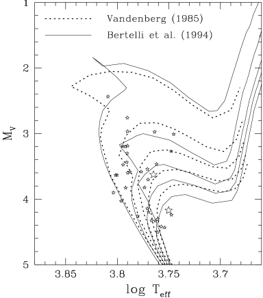
Fig. 1.: Comparison for [Fe/H]=0.0 between the Vdb85, LAOL based isochrones with the OPAL based isochrones from Bert94ea. The isochrones ages are 2, 4, 6, 8 and 10 Gyr for the LAOL based set and 2, 4, 6.3, 8 and 10 Gyr for the OPAL based set. The Vdb85 isochrones are shifted by $\delta\log T_{\rm eff}$ = –0.009 to satisfy the solar constraint (see Edv93ea for details). In addition, the stars (Table4) with metallicities $-0.05\!<\!{\rm[Fe/H]}\!<\!0.05$ have been inserted. The symbols are the same as those in the following figures

Note, that our fitting method is not substantially different from the determination of the age in the ($\log T_{\rm eff},\Delta M_{V}$) diagram used by Edv93ea. Since $\Delta M_{V,o}$ = $M_{V,o,zams}-M_{V,o}$ and $\Delta M_{V,i}$ = $M_{V,i,zams}-M_{V,i}$, then minimizing the difference between the observed and the isochrone magnitude implies: $\delta M_{V}=\Delta M_{V,o}-\Delta M_{V,i}$. With $M_{V,o,zams}=M_{V,i,zams}$ this equals to the quantity minimized in the reduced chi-squared defined above. If on the other hand $M_{V,o,zams}\neq M_{V,i,zams}$ then an unnecessary bias would have been added in the results. In that case minimization in the ($\log T_{\rm eff},M_{V}$) plane should be preferred over minimization in the ($\log T_{\rm eff},\Delta M_{V}$) plane.

2.2.3 Uncertainties in $T_{\rm eff}$, [Fe/H] & distance

The uncertainties in the effective temperature, metallicity and the distance will give different results for the fitted mass and age along the isochrone. For each star we repeated the calculations with slightly different values for the effective temperature (–50/+100K; see Edv93ea), the metallicity ($\pm 0.07$ in [Fe/H]; adopted) and the distance ($\pm 15\%$ for distances given by Edv93ea; in Tables7 & 8 the uncertainties are considered separately for each star with an Hipparcos parallax). In total 7 different values for the mass and the age of each star are obtained. A consequence of the automatic fitting procedure is that it always provides an answer, which sometimes is not a good fit to the actual data. The latter were not considered in the calculation of the unweighted mean and the uncertainty in the age and mass of each star in the sample.

Fig. 2.: A comparison between the ages from Tables3 & 4 with those determined by Edv93ea, due to different isochrone sets. The open circles denote the MS stars from Table3 and the asterisks denote the SGB stars from Table4. The big symbols are for stars with at least 6 out of the maximum 7 good age obtained from the analysis (see Sect.2.2.3 for details) and for which the uncertainty in $\rm\overline{log(age)}$ is smaller than 0.05. The small symbols are used in all remaining cases and refer in general to stars with less reliable ages

When various measures for a particular star of the V-band photometry were found in different databases the complete procedure as described above was applied for each photometric measurement. Then an average was computed, weighted over the photometric errors given by the various authors or adopted by us (0$\;.\!\!\!^{m}$01 for the photometry from the bright star catalogue and 0$\;.\!\!\!^{m}$05 if the photometric errors were not specified at all).

2.2.4 Isochrone population

The method thus far considers only the formal solution, automatically generated by the procedure outlined above. However, ambiguities in the age determinations are not taken into account when the stars are located near the end of the core-H burning phase. In the vicinity of the termination point (i.e. the hook feature) of young isochrones, it is possible that the star is either at the end of the main sequence phase or beyond the termination point, each implying a different value for the age of the star. In the mass range from 1.0 – 1.7M_⊙ the evolution along the SGB (Sub-Giant Branch) is roughly 4 – 40 times faster than the evolution from the ZAMS (Zero Age Main Sequence) up to the termination point. Evolved stars must therefore be inspected individually. If the resulting age results in a position on the isochrone beyond the termination point, then an alternative age corresponding to a point below the termination point is assigned to the star (see last column Table4).

Fig. 3.: The AMR for all the stars in Tables 3&4. See Fig.2 for the symbol description, but the small symbols are used here for the remaining cases with $n\!>\!2$ and an uncertainty in $\rm\overline{log(age)}\!<\!0.3$

Fig. 4.: (a) The AMR for the stars in Tables3&4 with a dispersion in $\rm\overline{log(age)}\!<\!0.05$ (see Fig.2 for the symbol description), (b) the AMR for the same stars, but now with the ‘visually’ assigned ages for the SGB stars (filled triangles, last column Table4), and (c) the AMR for the same stars, but now with the ages from Edv93ea.

2.2.5 The Lutz-Kelker correction

Lutz & Kelker (1973) demonstrated that a bias is present among stars with their absolute magnitudes obtained from trigonometric parallax. The bias is not confined to volume limited samples as discussed by Trumpler & Weaver (1953) and it depends only on the ratio ($\sigma_{\pi}/\pi$), i.e. the ratio of the standard error of the parallax over the parallax. Due to observational errors in the parallax one expects to find statistically more stars from a larger distance scattering into a smaller volume than vice versa. The consequence of this geometrical effect is that the stars in a sample are on average brighter and younger than they appear to be.

Thus far we have considered the formal uncertainties in the method to determine the age of the stars. Edv93ea compared their photometrically derived distances with those obtained from ground based parallaxes. They found an excellent agreement and estimated that the uncertainty in the distances is about 15%. Their à posteriori information about the compatibility with parallax data implies that we ought to apply a Lutz-Kelker correction in our analysis. This correction is in the generalized case only invoked by the relative uncertainties in the distance scale. Note however, that Edv93ea (p121 and references cited therein) do not have to apply a Lutz-Kelker correction, because the distances that we adopted from their paper were neither required or used in their $\Delta M_{V}$-method.

The Lutz-Kelker correction is applied to the absolute magnitudes determined from distances for the stars from Edv93ea. We expect, within the volume considered, a homogeneous distribution for the F- & G-type stars and we used Hanson’s equation 31 (Hanson 1979) with index $n\!=\!4$ to compute the value of the correction. The stars become about 0$\;.\!\!\!^{m}$3 brighter with $\sigma_{\pi}/\pi\!\simeq\!0.15$. The correction leads to negligible differences in the results with distances from the Hipparcos parallax, because for the majority of the stars $\sigma_{\pi}/\pi\!<\!0.03$.

2.3 Results

The results are presented in three stages. First, we show the differences due to a change of isochrones: Vdb85 versus Bert94ea. However, no corrections were made for a bias in the absolute magnitudes. This is done in the second stage of the analysis. In the third and final stage we based the analysis on the Hipparcos parallax.

Fig. 5.: A comparison of the ages computed with the distances of the stars based on Hipparcos parallaxes (Tables7 & 8). Panel (a) shows the comparison with the ages from Edv93ea. The differences are due to the isochrones and the fitting method. In panel (b) we make a comparison with the ages from Tables5 & 6. The differences are only due the distances adopted for the stars (photometric distances from Edv93ea with the Lutz-Kelker correction versus distances from trigonometric parallax). Symbols are the same as described in Fig.2

Fig. 6.: The AMR similar to Fig.3, but now for all the stars in Tables7 & 8 with their distances based on Hipparcos parallaxes (ESA 1997). See Fig.2 for the symbol description. Small symbols are used here for the remaining cases with $n\!>\!2$ and an uncertainty in $\rm\overline{log(age)}\!<\!0.3$

Table1 shows the sensitivity of the age through individual variation of each of the input parameters in comparison with the mean age obtained for each star. The first set of calculations show the sensitivity of the results for the uncertainties, as described in Sect.2.2.3, adopted for the input parameters. In the second & third set of calculations a smaller uncertainty in the distance was adopted and in the fourth set we further assumed smaller uncertainties in the effective temperature and metallicity. The average results, from the procedure outlined in preceding sections, are given in the Tables3 & 4. They list respectively the stars which are on or very near to the MS (Main Sequence) and those which are on the SGB. The Lutz-Kelker correction was not applied in order to discuss the effects from different sets of isochrones. Tables5 & 6 contain the ages when the correction is applied. Table 2 shows, similar to Table1, the sensitivity of the age through variation of the individual parameters, but now based on Hipparcos distances instead of the distances given by Edv93ea. The average results for each star (MS and SGB) are given in the Tables7 & 8.

In the following set of figures we first compare the difference due to a different choice of isochrones, i.e. Figs.2 – 4. Figs.5ab & 6 show the relations when the trigonometric parallaxes from Hipparcos are adopted. In Fig.2 we compare the ages for the stars computed with the Bert94ea isochrones with the ages given by Edv93ea. The comparison shows that towards older age the revised values are systematically larger than Edv93ea, see Sect.3.1 for a detailed discussion about this difference. Note that we refer to the stars with reliable ages, i.e. the big symbols, and discarded the old MS stars (small open circles) from the comparison. Figure3 shows the age-metallicity for all the stars listed in Tables3 & 4. Figure4a shows the AMR for the SGB stars with an average age obtained from at least six out of the maximum of seven good age determinations with an uncertainty in log(age) $<$ 0.05. Figures4b & 4c show for comparison the AMR for the same stars, but now with respectively the ‘visually’ assigned ages for the SGB stars (see also Sect.2.2.4) and the ages from Edv94ea. In Figs.5a & 5b we compare the ages (Tables7 & 8), based on absolute magnitudes obtained from Hipparcos parallaxes, with those obtained by Edv93ea and the ages given in Tables5 & 6. Figure6 is similar to Fig.3, but now the ages are based on the distances from the Hipparcos parallax instead of the distances given by Edv93ea. Figure7a displays the relation obtained from distances derived from the Hipparcos parallax, while Fig.7b shows for comparison the same stars, but now with the ages from Edv93ea.

3 Discussion

3.1 Revised ages

3.1.1 Isochrones

In Fig.2 a comparison is made between the ages obtained by Edv93ea and those determined here with the Bert94ea isochrones. The general trend is that the revised ages get systematically larger towards older ages. On the other hand, the revised ages of a few MS stars are found to be considerably younger, while a few other young MS stars are now considerably older. The general trend should mainly originate from the differences between the Vdb85 and Bert94ea isochrones. Differences in the opacities, initial abundance mix, and the different conversion tables have barely influence on the age obtained. $\bullet$ Convective overshoot is only present in stars with $M\!\geq\!1\;M_{\odot}$ or $t\!\mathrel{\mathchoice{\vbox{\offinterlineskip\halign{\hfil$\displaystyle#$\hfil\cr<\cr\sim\cr}}}{\vbox{\offinterlineskip\halign{\hfil$\textstyle#$\hfil\cr<\cr\sim\cr}}}{\vbox{\offinterlineskip\halign{\hfil$\scriptstyle#$\hfil\cr<\cr\sim\cr}}}{\vbox{\offinterlineskip\halign{\hfil$\scriptscriptstyle#$\hfil\cr<\cr\sim\cr}}}}\!10$Gyr (see Chiosi etal. 1992, Bert94ea, and references cited in those papers). The effect of convective overshoot at the MS is that the stars have larger cores. This results in a higher luminosity and a prolonged age. It should lead to systematically older ages for the stars with respect to ages determined from the Vdb85 isochrones. $\bullet$ The differences in the helium mass fraction has the following effect on the age determination:

• for solar metallicity isochrones the helium mass fraction $Y$ is lower in the Vdb85 isochrones; the effects of difference in $Y$ was checked with the isochrones present in our data base with ($Z$ = 0.05,$Y$ = 0.352) and ($Z$ = 0.05,$Y$ = 0.4, unpublished); a lower $Y$ leads to a lower $T_{\rm eff}$ due to an increased opacity from a higher hydrogen mass fraction $X$, while the turn-off luminosity remains comparable; as a result the MS turn-off ages determined with isochrones with a lower $Y$ will be younger; from this argument one expects older ages from the Bert94ea isochrones;

• for metal-poor isochrones $Y$ is higher in the Vdb85 isochrones; this leads to the reverse effect, i.e. younger ages from the Bert94ea isochrones.

The general trends outlined above are at young age not in agreement with Fig.2, because we expect older ages from the Bert94ea isochrones. Instead we find a comparable or even a slightly younger age. A similar discrepancy is found for old stars with relatively low metallicities. We further note, that the Vdb85 isochrones with [Fe/H] = 0.0 were not as expected from the difference in $Y$ located at lower, but higher effective temperature. In addition, the shift of $\delta\log T_{\rm eff}$ = $-\!0.009$ applied by Edv93ea to the Vdb85 isochrones makes it even more difficult to determine the origin of the differences between the Edv93ea and our revised ages. There are too many differences (e.g. opacities, convective overshoot, normalization, conversion tables …) between the Bert94ea and the Vdb85 isochrones that it is not only hard to compare them, but also to understand which of the differences or a combination of them is/are the dominant factor(s). All the factors mentioned above hamper the analysis on the origin of the differences between the Edv93ea and the revised ages. Although we are able to outline general differences between the re-normalized Vdb85 and Bert94ea isochrones, we fail to prove with plain arguments the exact differences between two isochrone sets and hence the differences between the ages obtained by Edv93ea and this work. To understand the difference between these isochrones requires a deep and detailed analysis of isochrones with the same $Y,Z$. Unfortunately they are not available to us, while their computation is beyond the scope of this paper.

3.1.2 Hipparcos parallaxes

Figure5a shows the effects due to differences in the isochrones and the fitting method. The reliable ages of the stars based on the Hipparcos parallax (the big symbols) get $\sim$ 2Gyr older for stars in the age spanning 9 – 16Gyr, $\sim$ 1Gyr older for stars in the age spanning 4 – 9Gyr, and a negligible difference for stars younger than 4Gyr. Figure 5b displays the effects due to differences in the distance: photometric distances from Edv93ea and the derived absolute magnitudes corrected for the Lutz-Kelker bias versus the distances derived from the Hipparcos parallax. It indicates that, besides some increased scatter, the ages based on the Hipparcos parallax are slightly younger for $t\!>\!8$Gyr.

Fig. 7.: (a) The AMR for the stars in Tables7 & 8 with a dispersion in $\rm\overline{log(age)}\!<\!0.05$ (see Fig.2 for the symbol description) and (b) the AMR for the same stars, but now with the ages from Edv93ea.

3.2 Sensitivity of the results

Table1 shows the results from four sets of calculations to check the sensitivity of the results caused by uncertainties in the input parameters. The mean age difference $\overline{\delta}$ gives the shift of the age due to variation of each of the input parameters. The variance $\sigma$ gives an indication about the scatter in the input parameter varied.

All sets of calculations indicate that both $\overline{\delta}$ and $\sigma$ are significantly larger for the MS stars. This shows that the stars which contribute mostly to a large age spread are automatically identified as MS stars. The analysis further shows that the 15% uncertainty in the distance of the SGB stars is the main cause of their large age spread. An uncertainty of 5% is required to obtain variances comparable to those obtained for the other input parameters. A better determination of $T_{\rm eff}$ and/or [Fe/H] does not lead to a significant improvement as long as the distances are not accurate down to a 5% level. Table2 shows that a slightly larger improvement is obtained when the Hipparcos parallaxes are used. A reduction of the uncertainty in the ages will not be obtained from even more accurate distances, but from a better definition of the effective temperatures for the stars in the sample. Figure7a further demonstrates that the number of stars with reliable ages has increased considerable with respect to the stars displayed in Fig.4a.

3.3 MS stars

Figures 3 and 6 show the age-metallicity of all the stars in the sample analysed. The uncertainties in the ages of old MS stars are quite large. Near the MS the evolution is quite slow and the isochrones of different ages are packed closely together. Small uncertainties in $\log T_{\rm eff},M_{V}$ or metallicity give rise to large differences in the age of the MS star. In the age-metallicity plane this results in an increased scatter of the MS stars. Edv93ea removed from their sample stars which lied too close to the ZAMS with errors log(age) $>$ 0.15. This is a subjective operation, because it partly depends on the exact definition of the ZAMS. As a consequence some MS might have been overlooked or too many taken out.

The older ages obtained by Edv93ea for some of the solar metallicity MS stars (see Figs.2 & 3) and the inclusion of these stars in the definition of the AMR results in a larger scatter in the definition of the disc AMR. The location of the MS turn-off tabulated by Bert94ea is used by us to distinguish a MS from a SGB star. In this way we classified more stars than Edv93ea as a MS star. The larger variance of the MS stars in Tables1 & 2 appears to justify the current approach. As argued in Sect.2.2.2 our fitting method is not substantially different from the one used by Edv93ea. The reason why they identified a different amount of stars too close to the MS is related to either of the following:

• the exact location of the ZAMS adopted in the definition of $\Delta M_{V}$ for different metallicities,

• a broader MS band due to convective overshoot.

To some extent a different choice of the isochrone with metallicity Z from a specific [Fe/H] or [Me/H] affects not only the age, but in our case also the distinction between MS or SGB star.

3.4 SGB stars

The situation changes if a star is on the SGB, where the evolution is relatively fast and the uncertainty in the age is considerably smaller. These stars potentially define a genuine disc AMR. Figure4a shows the AMR for the SGB stars. It still has a large scatter in age and/or metallicity, but there is definitely a small slope of $\sim$0.04 dex/Gyr present. For comparison we show in Fig.4b & 4c the AMR for the same stars, but now with respectively the visually assigned ages and the ages from Edv93ea. Figure4b has a similar slope, while Fig.4c shows an even steeper slope of $\sim$0.07 dex/Gyr. The latter slope is also obtained when the Lutz-Kelker correction is applied to the absolute magnitude of the stars prior to the computation of the age or when the distances are derived from the Hipparcos parallax, see Fig.7a. However, one should be aware of the caveat that the slope might be shallower. Because some old, metal-rich stars might be absent in the sample, due to the selection criteria used by Edv93ea.

Figures3, 4a – c, 6 and 7a & b indicate that there is no apparent AMR for stars with an age less than 10Gyr. We are basically dealing with a large metallicity spread among the stars. Only, if we consider the older stars a slope appears.

A comparison of Figs.4a & 4b further indicates that there is no significant difference in the AMR slope between the automatically determined ages and the visually improved ages of the SGB stars. Preference is given to the objectively determined ages for the SGB stars in Fig.4a, which have an uncertainty in their age of less than 12%, while the estimated uncertainty in the metallicity is smaller than 0.07dex. The slope in the AMR is not expected to be an artifact. The large spread in age and/or metallicity in Figs.4a and 7a & 7b is likely real. It could imply that the AMR in Fig.6 is a superposition of a multitude of relations due to in-fall or past mergers events.

Fig. 8.: The age-mass relation for the MS and SGB stars in Tables7 & 8 with an uncertainty in $\rm\overline{log(age)}\!<\!0.05$. The results were obtained with calculations based on the Hipparcos parallax. We refer to Fig.2 for the symbol description

3.5 Initial stellar masses

Figure8 displays the ages with the corresponding masses obtained for the reliable ($\sigma_{\tau}\!<\!0.05$) MS stars from Table7 and the SGB stars from Table8. One expects a smooth and continuous relation, but between 10 – 12Gyr there is a hint of a slight discrepancy in the distribution of the stars. It could be an indication that stars with a larger age are younger and/or that the stars with ages larger than $\sim$ 8Gyr are possibly slightly older. It might originate from the transition of isochrones with convective overshoot to isochrones without it, see Sect.3.1 for the discussion about the presence or absence of overshoot. On the other hand, some stars with ages $\mathrel{\mathchoice{\vbox{\offinterlineskip\halign{\hfil$\displaystyle#$\hfil\cr>\cr\sim\cr}}}{\vbox{\offinterlineskip\halign{\hfil$\textstyle#$\hfil\cr>\cr\sim\cr}}}{\vbox{\offinterlineskip\halign{\hfil$\scriptstyle#$\hfil\cr>\cr\sim\cr}}}{\vbox{\offinterlineskip\halign{\hfil$\scriptscriptstyle#$\hfil\cr>\cr\sim\cr}}}}$ 13Gyr could be systematically younger. Since the same procedure was applied to determine the age, the origin should be due to one or more input parameters, possibly a combination of [Fe/H] and $T_{\rm eff}$. However, [Fe/H] is likely the dominant factor. Moreover, at [Fe/H] $\mathrel{\mathchoice{\vbox{\offinterlineskip\halign{\hfil$\displaystyle#$\hfil\cr<\cr\sim\cr}}}{\vbox{\offinterlineskip\halign{\hfil$\textstyle#$\hfil\cr<\cr\sim\cr}}}{\vbox{\offinterlineskip\halign{\hfil$\scriptstyle#$\hfil\cr<\cr\sim\cr}}}{\vbox{\offinterlineskip\halign{\hfil$\scriptscriptstyle#$\hfil\cr<\cr\sim\cr}}}}$  – 0.4 Edv93ea found that the stars are relatively over-abundant in the $\alpha$ elements. In these cases we might have not used the optimum set of isochrones to determine the age, which results in a small discrepancy in both the older ages and the initial mass for these stars.

3.6 In summary

We have computed with the Bert94ea isochrones new ages for the stellar sample defined by Edv93ea. The revised values are systematically larger towards older ages. The differences are considerably smaller when the distances are based on the Hipparcos parallax. The stars on the SGB define a disc AMR with a slope of $\sim 0.07$ dex/Gyr. A comparable slope is obtained, when the Edv93ea ages are adopted for the same stars.

• A. Bressan, C. Chiosi and L. Girardi are acknowledged for their comments and discussions. We further thank the referee for his stimulating suggestions and critical notes, which lead, together with the comments made afterwards by Drs. B.Gustafsson, B.Edvardsson and P.E.Nissen to a substantial improvement of the presentation of the paper. Bertelli acknowledges the financial support received from the Italian Ministry of University, Scientific Research and Technology (MURST) and the National Council of Research. Ng is supported by TMR grant ERBFMRX-CT96-0086 from the European Community.

This article was processed by the author using Springer-Verlag LaTeX A&A style file L-AA version 3.

Table 3.: The age of F- and G-type on or very near the main sequence stars in the solar neighbourhood. The age is an average over the sensitivity analysis performed, see Sects.2.2.3 & 3.2 for additional details. Column1 gives the identifier of the star, columns2&3 give the mean mass & the standard deviation for this mean value, columns4&5 give the average age together with its standard deviation, and column6 shows the number of good fits (out of the maximum 7, see Sect.2.2.3) over which the average is obtained. In addition, $n\!=\!1$ indicates that 1 out of the 7 fits converged. The values in columns 2&4 refer to the good fit, while the standard deviation is in that case calculated over the ‘good’ (1) and ‘second best’ (6) estimates. A value $n\!=\!0$ indicates not a good fit was obtained in all 7 possible cases and the mean & standard deviation refer in this case to the ‘second best’ value

ID		m	$\sigma_{m}$	$\tau$	$\sigma_{\tau}$	$n$		ID		m	$\sigma_{m}$	$\tau$	$\sigma_{\tau}$	$n$
HR	140	1.31	0.04	9.293	0.115	7		HR	6315	1.14	0.03	9.365	0.254	6
HR	219	0.97	0.03	8.957	1.337	4		HR	6409	1.52	0.06	9.265	0.032	7
HR	370	1.21	0.04	9.502	0.053	7		HR	6775	0.89	0.03	9.965	0.182	7
HR	458	1.28	0.04	9.433	0.038	7		HR	6907	1.35	0.04	9.298	0.063	7
HR	672	1.25	0.07	9.572	0.102	6		HR	7126	1.43	0.03	8.916	0.263	7
HR	784	1.20	0.02	9.182	0.258	5		HR	7560	1.28	0.05	9.473	0.035	7
HR	799	1.21	0.03	9.227	0.282	6		HR	7955	1.34	0.05	9.421	0.030	7
HR	962	1.32	0.05	9.471	0.037	7		HR	8181	0.90	0.03	9.893	0.231	7
HR	1010	0.96	0.03	9.730	0.505	6		HR	8472	1.54	0.06	9.312	0.040	7
HR	1173	1.44	0.04	9.062	0.177	7		HR	8885	1.39	0.04	9.255	0.062	7
HR	1257	1.42	0.07	9.386	0.067	7		HD	6434	0.85	0.03	9.945	0.245	6
HR	1489	1.22	0.06	9.592	0.088	7		HD	17548	0.88	0.01	10.048	0.072	4
HR	1687	1.43	0.04	8.923	0.367	7		HD	22879	0.79	0.02	10.089	0.115	2
HR	1780	1.15	0.03	9.304	0.318	5		HD	25704	0.80	0.03	10.038	0.169	3
HR	1983	1.22	0.03	9.219	0.232	6		HD	30649	0.82	0.03	10.246	0.020	2
HR	2047	1.06	0.02	9.531	0.234	5		HD	43947	0.96	0.03	9.942	0.080	6
HR	2220	1.34	0.03	9.098	0.157	6		HD	51929	0.83	0.03	10.073	0.063	4
HR	2493	0.98	0.02	9.874	0.092	7		HD	62301	0.84	0.02	10.091	0.025	2
HR	2721	0.99	0.04	8.987	1.741	6		HD	66573	0.80	0.03	10.136	0.182	4
HR	2943	1.51	0.05	9.235	0.027	7		HD	69611	0.81	0.03	10.237	0.022	2
HR	3018	0.82	0.03	8.733	0.277	1		HD	74011	0.82	0.03	10.238	0.844	1
HR	3578	0.79	0.03	10.156	0.150	6		HD	78747	0.80	0.04	10.120	0.250	6
HR	3954	1.40	0.07	9.366	0.076	7		HD	89707	0.94	0.04	9.750	0.497	7
HR	4012	1.38	0.05	9.419	0.030	7		HD	91347	0.86	0.03	10.057	0.157	6
HR	4067	1.40	0.05	9.326	0.028	7		HD	98553	0.91	0.04	9.840	0.271	6
HR	4395	1.51	0.06	9.273	0.029	7		HD	114762	0.78	0.02	10.214	0.000	2
HR	4529	1.37	0.05	9.434	0.032	7		HD	126512	0.83	0.03	10.229	0.841	1
HR	4533	1.36	0.04	9.189	0.131	7		HD	134169	0.82	0.04	8.006	0.004	0
HR	4540	1.31	0.05	9.429	0.032	7		HD	148211	0.83	0.04	10.192	0.052	2
HR	4657	0.93	0.03	9.723	0.415	7		HD	148816	0.78	0.03	10.184	0.824	1
HR	4688	1.37	0.04	9.289	0.050	7		HD	155358	0.81	0.04	10.230	0.038	2
HR	4767	1.08	0.03	9.599	0.187	6		HD	165401	0.85	0.02	10.083	0.074	5
HR	4785	0.98	0.04	9.774	0.244	6		HD	174912	0.85	0.04	10.050	0.220	6
HR	4845	0.81	0.02	10.189	0.095	4		HD	184499	0.86	0.03	9.475	0.556	1
HR	4903	1.44	0.04	9.420	0.035	6		HD	199289	0.78	0.03	10.042	0.140	5
HR	5011	1.24	0.05	9.551	0.042	7		HD	201891	0.79	0.01	9.904	0.077	3
HR	5235	1.53	0.04	9.337	0.036	6		HD	208906	0.85	0.04	9.958	0.217	6
HR	5323	1.36	0.05	9.411	0.030	7		HD	210752	0.82	0.03	10.137	0.132	6
HR	5542	1.30	0.08	9.534	0.091	7		HD	215257	0.86	0.02	10.036	0.063	6
HR	5698	1.44	0.05	9.363	0.030	7		HD	218504	0.86	0.04	10.135	0.031	2
HR	6243	1.66	0.07	9.219	0.042	7

Table 4.: The age of F- and G-type sub-giant branch stars in the solar neighbourhood. See caption of Table3 for a description of columns1 – 6 and additional details. In addition, column7 refers to the visually assigned ages

ID		m	$\sigma_{m}$	$\tau$	$\sigma_{\tau}$	$n$	$\tau_{v}$		ID		m	$\sigma_{m}$	$\tau$	$\sigma_{\tau}$	$n$	$\tau_{v}$
HR	17	1.06	0.04	9.790	0.086	5	9.75		HR	5019	0.96	0.03	10.087	0.054	7	10.09
HR	33	1.09	0.03	9.774	0.057	6	9.68		HR	5338	1.32	0.04	9.517	0.032	6	9.45
HR	35	1.29	0.03	8.569	1.660	6	9.33		HR	5353	1.34	0.01	9.545	0.009	5	9.54
HR	107	1.22	0.06	9.550	0.106	7	9.50		HR	5423	1.22	0.12	9.695	0.153	3	9.70
HR	145	1.17	0.05	9.659	0.078	5	9.64		HR	5447	1.25	0.03	9.349	0.086	7	9.38
HR	203	1.00	0.04	9.975	0.062	7	9.98		HR	5459	1.00	0.02	9.928	0.087	5	9.89
HR	235	1.14	0.02	9.416	0.170	4	9.56		HR	5691	1.27	0.08	9.535	0.096	7	9.50
HR	244	1.31	0.05	9.497	0.069	7	9.45		HR	5723	1.46	0.07	9.341	0.067	7	9.32
HR	340	1.21	0.06	9.669	0.084	4	9.63		HR	5868	1.10	0.03	9.815	0.048	4	9.73
HR	366	1.24	0.07	9.522	0.115	7	9.47		HR	5914	0.86	0.03	10.163	0.039	3	10.20
HR	368	1.39	0.07	9.390	0.069	7	9.34		HR	5933	1.21	0.05	9.450	0.046	4	9.51
HR	448	1.24	0.06	9.645	0.067	7	9.50		HR	5968	0.93	0.03	10.083	0.042	6	10.10
HR	483	1.06	0.03	9.807	0.088	5	9.81		HR	5996	1.26	0.06	9.603	0.078	6	9.49
HR	573	1.08	0.03	9.717	0.079	6	9.72		HR	6189	1.04	0.04	9.829	0.051	6	9.69
HR	646	1.24	0.06	9.554	0.095	6	9.47		HR	6202	1.38	0.07	9.406	0.061	5	9.34
HR	720	1.01	0.04	9.958	0.051	7	9.96		HR	6458	0.88	0.03	10.169	0.817	1	10.26
HR	740	1.35	0.08	9.448	0.078	7	9.38		HR	6541	1.29	0.07	9.529	0.082	7	9.43
HR	1083	1.42	0.04	9.241	0.044	7	9.26		HR	6569	1.31	0.03	9.367	0.050	7	9.36
HR	1101	1.09	0.03	9.824	0.037	5	9.65		HR	6598	0.97	0.04	10.019	0.069	7	10.02
HR	1294	0.98	0.04	10.029	0.057	7	10.03		HR	6649	1.02	0.03	9.877	0.069	7	9.88
HR	1536	1.28	0.07	9.595	0.078	7	9.50		HR	6701	1.31	0.05	9.512	0.047	4	9.43
HR	1545	1.20	0.04	9.554	0.061	7	9.55		HR	6850	1.27	0.04	9.415	0.033	7	9.43
HR	1673	1.26	0.06	9.496	0.086	7	9.45		HR	7061	1.37	0.10	9.449	0.102	7	9.36
HR	1729	1.10	0.04	9.821	0.052	7	9.68		HR	7232	0.99	0.03	10.027	0.049	7	10.03
HR	2141	0.98	0.02	9.976	0.042	7	9.98		HR	7322	1.17	0.04	9.653	0.078	7	9.56
HR	2233	1.25	0.04	9.557	0.063	7	9.46		HR	7534	1.27	0.03	9.462	0.048	6	9.46
HR	2354	1.13	0.05	9.780	0.088	7	9.67		HR	7766	0.96	0.03	9.993	0.042	6	9.99
HR	2530	1.22	0.06	9.513	0.108	6	9.48		HR	7875	1.01	0.04	9.915	0.062	7	9.92
HR	2548	1.31	0.05	9.444	0.067	7	9.42		HR	8027	1.11	0.04	9.710	0.062	6	9.66
HR	2601	1.00	0.04	9.924	0.064	7	9.92		HR	8041	1.16	0.05	9.741	0.061	7	9.60
HR	2835	0.96	0.03	9.901	0.079	7	9.93		HR	8077	1.29	0.10	9.547	0.124	5	9.49
HR	2883	0.85	0.02	10.146	0.041	6	10.16		HR	8354	1.05	0.04	9.800	0.056	7	9.66
HR	2906	1.26	0.08	9.574	0.102	5	9.48		HR	8665	1.10	0.01	9.757	0.031	5	9.66
HR	3176	1.16	0.05	9.770	0.069	7	9.62		HR	8697	1.21	0.06	9.613	0.093	6	9.49
HR	3220	1.27	0.04	9.427	0.044	7	9.42		HR	8729	1.10	0.04	9.847	0.060	7	9.69
HR	3262	1.13	0.03	9.308	0.580	3	9.54		HR	8805	1.36	0.05	9.329	0.025	7	9.34
HR	3271	1.24	0.05	9.619	0.071	6	9.54		HR	8853	1.21	0.07	9.590	0.111	7	9.56
HR	3538	1.00	0.03	9.958	0.066	6	9.96		HR	8969	1.18	0.06	9.614	0.103	6	9.57
HR	3648	1.10	0.04	9.834	0.056	7	9.68		HD	2615	1.11	0.04	9.730	0.062	7	9.58
HR	3775	1.27	0.05	9.530	0.073	7	9.43		HD	14938	1.07	0.03	9.809	0.042	4	9.73
HR	3881	1.17	0.04	9.723	0.073	7	9.64		HD	18768	0.85	0.03	10.191	0.049	6	10.20
HR	3951	1.19	0.05	9.718	0.074	7	9.55		HD	38007	0.92	0.03	10.108	0.047	6	10.12
HR	4027	1.11	0.03	9.829	0.048	6	9.70		HD	68284	0.94	0.04	10.016	0.069	7	10.02
HR	4039	1.01	0.02	9.808	0.105	6	9.81		HD	78558	0.86	0.02	10.180	0.034	3	10.20
HR	4150	1.33	0.05	9.440	0.066	7	9.37		HD	130551	0.97	0.02	9.918	0.036	7	9.82
HR	4158	1.08	0.03	9.793	0.073	6	9.71		HD	144172	1.12	0.04	9.723	0.048	7	9.61
HR	4277	1.06	0.03	9.816	0.091	6	9.79		HD	157089	0.88	0.03	9.498	0.564	1	10.25
HR	4285	1.06	0.04	9.869	0.067	7	9.87		HD	159307	1.07	0.04	9.775	0.067	7	9.78
HR	4421	1.23	0.05	9.540	0.065	6	9.42		HD	188815	0.94	0.03	9.930	0.072	7	9.93
HR	4683	1.10	0.05	9.718	0.075	7	9.61		HD	198044	1.03	0.04	9.865	0.064	6	9.82
HR	4734	1.11	0.04	9.822	0.056	7	9.67		HD	200973	1.17	0.05	9.650	0.065	7	9.51
HR	4981	1.38	0.09	9.426	0.081	7	9.37		HD	201099	0.90	0.02	10.100	0.035	6	10.14
HR	4983	1.11	0.03	9.562	0.175	5	9.63		HD	205294	1.13	0.03	9.726	0.043	5	9.58
HR	4989	1.14	0.04	9.623	0.070	3	9.61		HD	221830	0.86	0.03	10.195	0.046	6	10.20

Table 5.: Similar to Table 3, but now with the Lutz-Kelker (1973) correction ($n$ = 4, $\sigma_{\pi}/\pi$ = 0.15; Hanson 1979, equation 31) applied to the absolute magnitude of the F- and G-type stars on or near the main sequence prior to the calculation of the age

ID		m	$\sigma_{m}$	$\tau$	$\sigma_{\tau}$	$n$		ID		m	$\sigma_{m}$	$\tau$	$\sigma_{\tau}$	$n$
HR	140	1.36	0.05	9.344	0.030	7		HR	5542	1.36	0.08	9.485	0.076	7
HR	219	0.96	0.03	9.814	0.197	6		HR	5698	1.50	0.07	9.333	0.051	7
HR	370	1.27	0.05	9.495	0.037	7		HR	5723	1.55	0.10	9.288	0.086	7
HR	458	1.35	0.05	9.419	0.030	7		HR	6243	1.73	0.05	9.175	0.034	6
HR	672	1.34	0.06	9.487	0.051	5		HR	6409	1.60	0.06	9.223	0.037	7
HR	784	1.23	0.03	9.298	0.289	7		HR	6907	1.41	0.05	9.318	0.028	7
HR	962	1.39	0.05	9.433	0.033	7		HR	7061	1.51	0.06	9.327	0.037	7
HR	1010	0.96	0.03	9.952	0.091	7		HR	7126	1.48	0.04	9.074	0.130	7
HR	1173	1.50	0.05	9.158	0.046	7		HR	7560	1.34	0.05	9.445	0.034	7
HR	1257	1.50	0.06	9.334	0.051	7		HR	7955	1.40	0.05	9.396	0.030	7
HR	1489	1.28	0.07	9.542	0.088	6		HR	8181	0.90	0.01	9.990	0.051	3
HR	1687	1.48	0.05	9.115	0.073	7		HR	8472	1.61	0.05	9.268	0.036	6
HR	2220	1.38	0.04	9.215	0.087	7		HR	8885	1.45	0.05	9.274	0.027	7
HR	2721	0.98	0.03	9.776	0.304	7		HD	6434	0.86	0.02	10.065	0.054	4
HR	2943	1.59	0.06	9.207	0.031	7		HD	22879	0.78	0.03	10.166	0.818	1
HR	3018	0.80	0.04	8.754	0.285	0		HD	25704	0.76	0.01	10.272	0.004	2
HR	3578	0.80	0.02	10.176	0.020	2		HD	51929	0.84	0.02	10.114	0.026	2
HR	3954	1.49	0.06	9.314	0.033	7		HD	62301	0.86	0.02	10.155	0.039	2
HR	4012	1.46	0.06	9.379	0.035	7		HD	66573	0.79	0.02	10.246	0.000	2
HR	4067	1.48	0.06	9.305	0.031	7		HD	78747	0.80	0.02	10.192	0.000	2
HR	4395	1.59	0.06	9.230	0.036	7		HD	98553	0.90	0.03	10.008	0.158	7
HR	4529	1.44	0.05	9.395	0.035	7		HD	114762	0.82	0.03	10.203	0.831	1
HR	4533	1.42	0.05	9.258	0.042	7		HD	134169	0.82	0.03	10.209	0.056	2
HR	4540	1.37	0.05	9.410	0.029	7		HD	148816	0.84	0.02	9.728	0.652	1
HR	4688	1.44	0.05	9.296	0.030	7		HD	174912	0.86	0.01	10.123	0.044	3
HR	4785	0.97	0.03	9.916	0.136	7		HD	199289	0.82	0.02	9.866	0.039	1
HR	4845	0.81	0.03	10.242	0.017	2		HD	201891	0.79	0.04	9.856	0.364	3
HR	4981	1.50	0.06	9.334	0.044	7		HD	208906	0.83	0.03	10.082	0.140	6
HR	5011	1.29	0.07	9.522	0.075	5		HD	210752	0.84	0.02	10.158	0.023	3
HR	5235	1.56	0.08	9.316	0.072	3		HD	215257	0.87	0.02	10.061	0.011	2
HR	5323	1.43	0.05	9.379	0.031	7

Table 6.: Similar to Table 5, but now for F- and G-type stars on the sub-giant branch

ID		m	$\sigma_{m}$	$\tau$	$\sigma_{\tau}$	$n$		ID		m	$\sigma_{m}$	$\tau$	$\sigma_{\tau}$	$n$
HR	17	1.10	0.04	9.749	0.061	5		HR	368	1.47	0.10	9.342	0.084	7
HR	33	1.14	0.06	9.724	0.072	4		HR	448	1.32	0.06	9.556	0.063	7
HR	35	1.33	0.04	9.322	0.039	6		HR	483	1.08	0.03	9.842	0.054	7
HR	107	1.26	0.06	9.516	0.093	6		HR	573	1.10	0.04	9.736	0.065	6
HR	145	1.18	0.06	9.677	0.092	6		HR	646	1.29	0.05	9.501	0.046	4
HR	203	1.05	0.04	9.906	0.057	6		HR	720	1.06	0.04	9.884	0.064	7
HR	235	1.15	0.02	9.577	0.116	6		HR	740	1.45	0.10	9.366	0.087	7
HR	244	1.35	0.06	9.491	0.060	7		HR	799	1.23	0.03	9.369	0.164	7
HR	340	1.37	0.07	9.468	0.054	3		HR	1083	1.48	0.05	9.251	0.022	7
HR	366	1.30	0.07	9.471	0.080	7		HR	1101	1.14	0.04	9.761	0.054	4

Table 6.: Continued …

ID		m	$\sigma_{m}$	$\tau$	$\sigma_{\tau}$	$n$		ID		m	$\sigma_{m}$	$\tau$	$\sigma_{\tau}$	$n$
HR	1294	1.03	0.05	9.950	0.069	6		HR	6202	1.45	0.09	9.354	0.074	5
HR	1536	1.34	0.06	9.532	0.062	6		HR	6315	1.16	0.03	9.512	0.136	7
HR	1545	1.21	0.04	9.583	0.076	6		HR	6458	0.89	0.03	10.162	0.047	6
HR	1673	1.31	0.08	9.471	0.091	7		HR	6541	1.33	0.05	9.491	0.049	5
HR	1729	1.14	0.03	9.784	0.046	6		HR	6569	1.38	0.04	9.347	0.045	7
HR	1780	1.18	0.03	9.504	0.127	7		HR	6598	1.03	0.05	9.918	0.080	7
HR	1983	1.25	0.03	9.357	0.141	7		HR	6649	1.04	0.04	9.864	0.046	7
HR	2047	1.08	0.03	9.421	0.662	5		HR	6701	1.35	0.05	9.482	0.051	5
HR	2141	1.01	0.03	9.944	0.040	6		HR	6775	0.90	0.01	10.030	0.045	2
HR	2233	1.32	0.07	9.487	0.072	7		HR	6850	1.32	0.07	9.410	0.083	7
HR	2354	1.17	0.05	9.729	0.063	7		HR	7232	1.04	0.04	9.957	0.063	7
HR	2493	0.98	0.03	9.932	0.054	5		HR	7322	1.20	0.06	9.620	0.095	6
HR	2530	1.24	0.06	9.522	0.087	6		HR	7534	1.31	0.05	9.451	0.059	7
HR	2548	1.35	0.09	9.437	0.086	7		HR	7766	1.00	0.04	9.940	0.052	7
HR	2601	1.05	0.04	9.838	0.068	7		HR	7875	1.06	0.04	9.847	0.052	6
HR	2835	0.97	0.03	9.921	0.046	6		HR	8027	1.13	0.03	9.711	0.044	7
HR	2883	0.89	0.02	10.078	0.045	6		HR	8041	1.23	0.05	9.656	0.067	7
HR	2906	1.32	0.06	9.520	0.059	7		HR	8077	1.32	0.09	9.529	0.098	7
HR	3176	1.23	0.06	9.673	0.075	7		HR	8354	1.11	0.05	9.720	0.069	6
HR	3220	1.32	0.05	9.428	0.067	7		HR	8665	1.16	0.05	9.693	0.080	6
HR	3262	1.15	0.03	9.548	0.120	3		HR	8697	1.26	0.05	9.566	0.065	4
HR	3271	1.31	0.06	9.557	0.064	5		HR	8729	1.17	0.05	9.757	0.071	7
HR	3538	1.03	0.03	9.946	0.044	7		HR	8805	1.42	0.07	9.340	0.069	7
HR	3648	1.15	0.03	9.772	0.048	6		HR	8853	1.24	0.06	9.585	0.092	7
HR	3775	1.33	0.10	9.483	0.092	6		HR	8969	1.23	0.04	9.583	0.073	5
HR	3881	1.19	0.04	9.706	0.055	5		HD	2615	1.17	0.05	9.640	0.073	7
HR	3951	1.26	0.05	9.631	0.064	6		HD	14938	1.10	0.04	9.771	0.052	7
HR	4027	1.16	0.06	9.758	0.079	6		HD	17548	0.87	0.02	10.111	0.040	7
HR	4039	1.03	0.04	9.855	0.072	6		HD	18768	0.89	0.04	10.115	0.074	7
HR	4150	1.42	0.08	9.376	0.071	7		HD	30649	0.86	0.02	10.185	0.040	2
HR	4158	1.11	0.03	9.761	0.038	7		HD	38007	0.97	0.04	10.035	0.074	7
HR	4277	1.08	0.04	9.833	0.082	7		HD	43947	0.99	0.04	9.957	0.068	7
HR	4285	1.11	0.04	9.796	0.056	6		HD	68284	1.00	0.05	9.917	0.078	7
HR	4421	1.29	0.06	9.472	0.074	6		HD	69611	0.86	0.02	10.175	0.040	2
HR	4657	0.92	0.02	9.926	0.079	7		HD	74011	0.83	0.02	10.224	0.046	5
HR	4683	1.14	0.05	9.676	0.059	6		HD	78558	0.90	0.02	10.107	0.048	6
HR	4734	1.17	0.05	9.742	0.067	7		HD	89707	0.93	0.02	9.979	0.080	6
HR	4767	1.09	0.02	9.689	0.110	6		HD	91347	0.89	0.01	10.083	0.060	2
HR	4903	1.46	0.06	9.416	0.068	6		HD	126512	0.84	0.02	10.214	0.045	5
HR	4983	1.14	0.03	9.600	0.072	6		HD	130551	1.00	0.03	9.881	0.045	7
HR	4989	1.17	0.04	9.643	0.074	7		HD	144172	1.17	0.04	9.653	0.059	7
HR	5019	1.00	0.03	10.028	0.048	6		HD	148211	0.86	0.02	10.146	0.043	6
HR	5338	1.44	0.06	9.420	0.050	5		HD	155358	0.84	0.02	10.184	0.042	5
HR	5353	1.43	0.12	9.468	0.102	3		HD	157089	0.87	0.03	10.155	0.046	6
HR	5423	1.33	0.01	9.557	0.009	4		HD	159307	1.12	0.04	9.700	0.054	6
HR	5447	1.30	0.04	9.357	0.033	7		HD	165401	0.89	0.02	9.997	0.028	2
HR	5459	1.04	0.03	9.912	0.046	5		HD	184499	0.84	0.03	10.203	0.049	6
HR	5691	1.31	0.06	9.524	0.065	7		HD	188815	0.96	0.02	9.938	0.037	7
HR	5868	1.13	0.04	9.780	0.056	7		HD	198044	1.05	0.03	9.849	0.044	6
HR	5914	0.89	0.03	10.115	0.044	6		HD	200973	1.25	0.03	9.544	0.031	5
HR	5933	1.24	0.06	9.528	0.098	6		HD	201099	0.92	0.03	10.066	0.050	7
HR	5968	0.97	0.04	10.037	0.055	7		HD	205294	1.22	0.04	9.611	0.053	6
HR	5996	1.35	0.08	9.521	0.073	6		HD	218504	0.88	0.02	10.105	0.043	6
HR	6189	1.11	0.05	9.744	0.065	7		HD	221830	0.90	0.04	10.112	0.064	7

Table 7.: The age of F- and G-type on or very near the main sequence stars in the solar neighbourhood. The age is an average over the sensitivity analysis performed, see Sects.2.2.3 & 3.2 for additional details. The distances of the stars are based on the Hipparcos parallax (ESA 1997). Column1 gives the identifier of the star, columns2&3 give the mean mass & the standard deviation for this mean value, columns4&5 give the average age together with its standard deviation, and column6 shows the number of good fits (out of the maximum 7, see Sect.2.2.3) over which the average is obtained. In addition, $n\!=\!1$ indicates that 1 out of the 7 fits converged. The values in columns 2&4 refer to the good fit, while the standard deviation is in that case calculated over the ‘good’ (1) and ‘second best’ (6) estimates. A value $n\!=\!0$ indicates not a good fit was obtained in all 7 possible cases and the mean & standard deviation refer in this case to the ‘second best’ value

ID		m	$\sigma_{m}$	$\tau$	$\sigma_{\tau}$	$n$		ID		m	$\sigma_{m}$	$\tau$	$\sigma_{\tau}$	$n$
HR	140	1.28	0.01	9.293	0.091	7		HR	5235	1.55	0.07	9.333	0.072	5
HR	219	0.95	0.02	9.911	0.094	7		HR	5323	1.42	0.01	9.386	0.017	7
HR	235	1.14	0.03	8.995	0.456	6		HR	5338	1.48	0.06	9.382	0.052	5
HR	458	1.29	0.01	9.438	0.034	7		HR	5542	1.30	0.06	9.529	0.085	7
HR	483	1.04	0.04	9.762	0.188	3		HR	5698	1.60	0.01	9.267	0.015	7
HR	672	1.22	0.04	9.584	0.082	7		HR	5723	1.54	0.02	9.280	0.015	7
HR	784	1.20	0.01	8.641	0.317	3		HR	6243	1.79	0.02	9.144	0.016	7
HR	962	1.32	0.01	9.471	0.024	7		HR	6315	1.14	0.02	9.448	0.138	7
HR	1010	0.98	0.03	9.544	0.499	6		HR	6409	1.72	0.02	9.163	0.015	7
HR	1173	1.45	0.01	9.128	0.052	7		HR	6458	0.86	0.01	8.006	0.002	0
HR	1257	1.49	0.03	9.346	0.034	7		HR	6907	1.39	0.01	9.326	0.030	7
HR	1294	0.94	0.02	10.036	0.061	2		HR	7126	1.43	0.01	8.977	0.106	7
HR	1687	1.46	0.01	9.113	0.055	7		HR	7232	0.95	0.03	9.874	0.227	7
HR	1780	1.15	0.02	9.285	0.328	7		HR	7560	1.23	0.01	9.496	0.047	7
HR	1983	1.22	0.02	9.131	0.247	7		HR	7955	1.61	0.01	9.270	0.014	7
HR	2047	1.09	0.03	7.693	1.972	3		HR	8181	0.89	0.02	10.004	0.069	6
HR	2220	1.32	0.02	7.794	2.711	7		HR	8472	1.58	0.01	9.286	0.014	7
HR	2493	0.97	0.02	9.890	0.061	7		HR	8885	1.50	0.02	9.268	0.021	7
HR	3018	0.83	0.00	8.004	0.001	0		HD	6434	0.86	0.01	10.094	0.031	4
HR	3538	1.00	0.02	9.669	0.245	6		HD	17548	0.87	0.02	10.078	0.055	4
HR	3578	0.85	0.02	9.101	0.414	1		HD	22879	0.79	0.00	9.584	0.599	1
HR	3954	1.59	0.02	9.255	0.017	7		HD	25704	0.83	0.01	8.004	0.003	0
HR	4012	1.58	0.02	9.299	0.020	7		HD	30649	0.85	0.01	8.005	0.002	0
HR	4039	1.02	0.04	9.830	0.087	6		HD	43947	0.96	0.03	9.959	0.073	7
HR	4067	1.47	0.01	9.310	0.021	7		HD	51929	0.86	0.01	8.886	0.335	0
HR	4395	1.26	0.01	8.005	0.002	0		HD	66573	0.79	0.02	10.264	0.051	3
HR	4529	1.39	0.01	9.428	0.018	7		HD	78747	0.80	0.02	10.239	0.049	3
HR	4533	1.33	0.01	9.140	0.104	7		HD	91347	0.86	0.02	10.105	0.074	5
HR	4540	1.30	0.01	9.433	0.033	7		HD	98553	0.91	0.03	9.818	0.221	7
HR	4657	0.92	0.02	9.895	0.084	6		HD	114762	0.82	0.03	10.202	0.829	1
HR	4688	1.47	0.02	9.293	0.026	7		HD	148816	0.82	0.00	10.211	0.003	2
HR	4767	1.08	0.03	9.270	0.347	6		HD	165401	0.85	0.01	10.109	0.045	7
HR	4785	0.97	0.03	9.855	0.128	7		HD	174912	0.83	0.03	10.151	0.087	7
HR	4845	0.81	0.02	10.233	0.059	3		HD	199289	0.79	0.01	8.003	0.002	0
HR	4903	1.44	0.05	9.422	0.048	7		HD	201891	0.79	0.01	8.003	0.003	0
HR	4981	1.48	0.05	9.348	0.046	7		HD	208906	0.82	0.02	10.140	0.064	6
HR	4983	1.11	0.02	9.208	0.265	6		HD	210752	0.85	0.01	10.113	0.797	1
HR	5019	0.92	0.03	9.955	0.151	7		HD	215257	0.88	0.01	10.073	0.011	2

Table 8.: The age of F- and G-type sub-giant branch stars in the solar neighbourhood. See caption of Table7 for additional details

ID		m	$\sigma_{m}$	$\tau$	$\sigma_{\tau}$	$n$		ID		m	$\sigma_{m}$	$\tau$	$\sigma_{\tau}$	$n$
HR	17	1.08	0.03	9.785	0.056	6		HR	5691	1.26	0.05	9.581	0.064	7
HR	33	1.08	0.01	9.796	0.023	6		HR	5868	1.08	0.04	9.809	0.085	6
HR	35	1.27	0.02	9.133	0.174	7		HR	5914	0.97	0.01	9.982	0.013	7
HR	107	1.21	0.05	9.556	0.101	7		HR	5933	1.20	0.01	9.509	0.049	5
HR	145	1.10	0.01	9.778	0.018	7		HR	5968	0.93	0.02	10.088	0.030	7
HR	203	1.03	0.02	9.926	0.022	7		HR	5996	1.10	0.04	9.755	0.103	7
HR	244	1.25	0.04	9.524	0.083	7		HR	6189	1.09	0.01	9.769	0.020	5
HR	340	1.75	0.03	9.122	0.026	0		HR	6202	1.38	0.06	9.408	0.048	7
HR	366	1.22	0.05	9.558	0.103	7		HR	6541	1.30	0.05	9.524	0.060	6
HR	368	1.46	0.04	9.341	0.038	7		HR	6569	1.32	0.01	9.351	0.022	7
HR	370	1.15	0.02	9.451	0.127	7		HR	6598	1.11	0.01	9.800	0.011	4
HR	448	1.18	0.01	9.724	0.020	7		HR	6649	1.05	0.02	9.863	0.020	6
HR	573	1.07	0.02	9.697	0.058	6		HR	6701	1.37	0.01	9.460	0.006	7
HR	646	1.26	0.04	9.548	0.068	6		HR	6775	0.90	0.02	10.067	0.034	7
HR	720	1.10	0.02	9.833	0.021	7		HR	6850	1.28	0.01	9.409	0.025	6
HR	740	1.40	0.05	9.391	0.059	6		HR	7061	1.33	0.04	9.486	0.059	7
HR	799	1.20	0.02	9.283	0.174	7		HR	7322	1.27	0.05	9.544	0.067	6
HR	1083	1.38	0.01	9.232	0.043	7		HR	7534	1.26	0.01	9.463	0.033	7
HR	1101	1.10	0.01	9.812	0.021	7		HR	7766	1.01	0.02	9.937	0.026	7
HR	1489	1.12	0.02	9.553	0.159	5		HR	7875	1.10	0.01	9.783	0.014	6
HR	1536	1.16	0.05	9.706	0.101	7		HR	8027	1.10	0.03	9.753	0.053	6
HR	1545	1.18	0.02	9.554	0.034	6		HR	8041	1.06	0.03	9.864	0.080	7
HR	1673	1.24	0.06	9.545	0.106	7		HR	8077	1.26	0.04	9.586	0.050	6
HR	1729	1.05	0.03	9.864	0.065	3		HR	8354	1.03	0.02	9.822	0.020	7
HR	2141	0.99	0.02	9.975	0.033	6		HR	8665	1.17	0.01	9.681	0.016	3
HR	2233	1.30	0.04	9.513	0.048	6		HR	8697	1.22	0.01	9.613	0.017	6
HR	2354	1.08	0.03	9.840	0.063	7		HR	8729	1.01	0.01	9.880	0.036	4
HR	2530	1.19	0.02	9.503	0.034	6		HR	8805	1.36	0.01	9.337	0.024	7
HR	2548	1.30	0.03	9.439	0.070	7		HR	8853	1.15	0.02	9.526	0.130	5
HR	2601	1.19	0.02	9.630	0.022	6		HR	8969	1.19	0.05	9.629	0.104	7
HR	2721	1.47	0.02	9.367	0.012	4		HD	2615	1.08	0.02	9.767	0.031	7
HR	2835	0.96	0.03	9.920	0.065	7		HD	14938	1.07	0.02	9.816	0.028	6
HR	2883	0.94	0.01	9.994	0.019	7		HD	18768	1.00	0.02	9.914	0.026	7
HR	2906	1.43	0.05	9.414	0.037	5		HD	38007	1.04	0.02	9.917	0.028	6
HR	2943	1.49	0.01	9.242	0.030	6		HD	62301	0.85	0.01	10.165	0.023	7
HR	3176	1.16	0.01	9.770	0.020	7		HD	68284	1.02	0.03	9.883	0.048	7
HR	3220	1.28	0.06	9.473	0.104	7		HD	69611	0.84	0.01	10.215	0.025	4
HR	3262	1.14	0.02	9.526	0.094	6		HD	74011	0.84	0.02	10.202	0.025	7
HR	3271	1.26	0.05	9.603	0.068	5		HD	78558	0.85	0.01	10.213	0.018	3
HR	3648	1.09	0.01	9.854	0.021	7		HD	89707	0.93	0.02	9.972	0.078	5
HR	3775	1.41	0.05	9.414	0.061	6		HD	126512	0.88	0.02	10.136	0.023	7
HR	3881	1.10	0.01	9.821	0.027	7		HD	130551	0.97	0.02	9.923	0.029	7
HR	3951	1.02	0.02	9.854	0.083	6		HD	134169	0.87	0.02	10.117	0.034	7
HR	4027	1.04	0.01	9.929	0.027	7		HD	144172	1.13	0.02	9.715	0.021	7
HR	4150	1.31	0.05	9.459	0.083	7		HD	148211	0.86	0.02	10.152	0.028	7
HR	4158	1.08	0.04	9.785	0.087	7		HD	155358	0.84	0.01	10.176	0.024	7
HR	4277	1.05	0.02	9.801	0.076	5		HD	157089	0.87	0.01	10.153	0.023	7
HR	4285	1.31	0.02	9.506	0.013	3		HD	159307	1.08	0.03	9.745	0.038	6
HR	4421	1.17	0.04	9.583	0.085	7		HD	184499	0.84	0.01	10.211	0.019	7
HR	4683	1.09	0.04	9.737	0.063	7		HD	188815	0.98	0.02	9.932	0.024	6
HR	4734	1.04	0.03	9.894	0.077	7		HD	198044	1.03	0.03	9.865	0.067	7
HR	4989	1.15	0.00	9.622	0.016	2		HD	200973	1.14	0.04	9.696	0.054	6
HR	5011	1.16	0.01	9.593	0.053	7		HD	201099	0.90	0.01	10.096	0.023	7
HR	5353	1.06	0.01	9.922	0.024	7		HD	205294	1.14	0.02	9.718	0.024	5
HR	5423	0.94	0.01	10.098	0.041	7		HD	218504	0.87	0.02	10.130	0.031	6
HR	5447	1.22	0.02	9.246	0.119	6		HD	221830	0.84	0.01	10.235	0.024	5
HR	5459	1.01	0.03	9.914	0.079	7

References

- 1992 Bertelli G., Bressan A., Chiosi C., Fagotto F., Nasi E., 1994, A&AS 106, 275 (Bert94ea)
- 1992 Chiosi C., Bertelli G., Bressan A., 1992, ARA&A 30, 235
- 1993 Edvardsson B., Andersen J., Gustafsson B., etal., 1993, A&A 275, 101 (Edv93ea)
- 1997 ESA, 1997, The Hipparcos and Tycho Catalogue, ESA SP-1200
- 1991 Grevesse N., 1991, A&A 242, 488
- 1976 Grønbech B., Olsen E.H., 1976, A&AS 25, 213
- 1979 Hanson R.B., 1979, MNRAS 186, 875
- 1991 Hoffleit D., Warren Jr. W.H., 1991, Bright Star Catalogue (5th revised edition)
- 1977 Huebner W.F., Merts A.L., Magee N.H., Argo M.F., 1977, Los Alamos Scientific Laboratory Report LA-6760-M
- 1992 Iglesias C.A., Rodgers F.J., Wilson B.G., 1992, ApJ 397, 717
- Lutz T.E., Kelker D.H., 1973, PASP 85, 573
- 1983 Olsen, E.H., 1983, A&AS 54, 55
- 1993 Olsen, E.H., 1993, A&AS 102, 89
- 1989 Pagel B.E.J., 1989, in ‘Evolutionary phenomena in Galaxies’, J. Beckman and B.E.J. Pagel (eds.), Cambridge University Press, 201
- 1987 Perry C.L., Olsen, E.H., Crawford D.L., 1987, PASP 99, 1184
- 1986 Press W.H., etal., 1986, Numerical Recipes
- 1992 Rodgers F.J., Iglesias C.A., 1992, ApJS 79, 507
- 1988 Schuster W.J., Nissen P.E., 1988, A&AS 73, 225
- 1953 Trumpler R.J., Weaver H.F., 1953, Statistical Astronomy, University of California Press (Berkeley), 368
- 1983 Vandenberg D.A., 1983, ApJS 51, 29
- 1985 Vandenberg D.A., 1985, ApJS 58, 711 (Vdb85)