Limits on Cosmological Models From
Radio-Selected Gravitational Lenses

Abstract

We are conducting a redshift survey of 177 flat-spectrum radio sources in 3 samples covering the 5 GHz flux ranges 50–100, 100–200 and 200–250 mJy. So far, we have measured 124 redshifts with completenesses of 80%, 68% and 58% for the bright, intermediate, and faint flux ranges. Using the newly determined redshift distribution we can derive cosmological limits from the statistics of the 6 gravitational lenses in the JVAS sample of 2500 flat-spectrum radio sources brighter than 200 mJy at 5 GHz. For flat cosmological models with a cosmological constant, the limit using only radio data is $\Omega_{0}>0.27$ at 2$-\sigma$ ($0.47<\Omega_{0}<1.38$ at 1$-\sigma$). The limits are statistically consistent with those for lensed quasars, and the combined radio + optical sample requires $\Omega_{0}>0.38$ at 2$-\sigma$ ($0.64<\Omega_{0}<1.66$ at 1$-\sigma$) for our most conservative redshift completeness model and assuming that there are no quasar lenses produced by spiral galaxies. Our best fit model improves by approximately 1$-\sigma$ if extinction in the early-type galaxies makes the lensed quasars fainter by $\Delta m=0.58\pm 0.45$ mag, but we still find a limit of $\Omega_{0}>0.26$ at 2$-\sigma$ in flat cosmologies. The increasing fraction of radio galaxies as compared to quasars at fainter radio fluxes (rising from $\sim$10% at 1 Jy to $\sim$50% at 0.1 Jy) explains why lensed optical emission is common for radio lenses and partly explains the red color of radio-selected lenses.

1 Introduction

The global geometry of the universe, usually specified by its matter density $\Omega_{0}$ and a cosmological constant $\lambda_{0}$, remains a significant source of uncertainty in cosmology. Current summaries of the constraints (e.g., Ostriker & Steinhardt 1995; Krauss & Turner 1995) favor a low matter density ($\Omega_{0}\sim 0.3$) either with or without a cosmological constant. The expectations of a low matter density are driven by observations of large-scale structure, the cluster baryon fraction, and nucleosynthesis (e.g., Peacock & Dodds 1994; White et al. 1993; Copi, Schramm & Turner 1995). Globular cluster ages, however, no longer require a low $\Omega_{0}$ due to the Hipparcos revisions of the distance scale (e.g. Chaboyer et al. 1997). A flat (inflationary) model would then require a cosmological constant $\lambda_{0}\sim 0.7$.

The number of gravitational lenses found in systematic surveys for lenses is a strong constraint on cosmological models, particularly models with a large cosmological constant (Turner 1990; Fukugita, Futamase & Kasai 1990). Quantitative analyses of surveys for multiply imaged quasars (Kochanek 1993, 1996a; Maoz & Rix 1993) currently give a formal two-standard deviation (2$-\sigma$) upper limit on the cosmological constant in flat models ($\Omega_{0}+\lambda_{0}=1$) of $\lambda_{0}<0.66$, and the lensing constraints are almost identical to the very preliminary results using Type Ia supernovae by Perlmutter et al. (1997). The statistical uncertainties are dominated by the Poisson errors from the small number of lensed quasars and the uncertainties in the local number counts of galaxies by type. The limits are also subject to several systematic errors; the principal ones are extinction (e.g. Kochanek 1991, 1996a; Tomita 1995; Malhotra, Rhoads & Turner 1996; Perna, Bartelmann & Loeb 1997), galaxy evolution (e.g. Mao 1991; Mao & Kochanek 1994; Rix et al. 1994), the quasar discovery process (Kochanek 1991), and the model for the lens galaxies (e.g., Maoz & Rix 1993; Kochanek 1993, 1994, 1996a).

We can eliminate two of these systematic errors, extinction and the quasar discovery process, by using the statistics of radio-selected lenses to constrain the cosmological model. Radio-selected lenses are immune to extinction in the lens galaxy, and radio lens searches work from flux-limited surveys that avoid the complicated systematic and completeness issues of quasar catalogs. Agreement between the optical and radio samples is a powerful check on some aspects of the lens galaxy models and for unanticipated systematic errors due to the large differences of the two samples in their redshift distributions, luminosity functions, and fractions of lensed objects. Moreover, we can reduce the Poisson uncertainties by performing a joint analysis if the samples are statistically consistent.

Unfortunately, the radio lens surveys use flux limits where there is little direct information on the source redshift distribution. Complete redshift surveys exist only for sources brighter than $>300$ mJy (e.g. the CJI/CJII samples, Henstock et al. 1995; the Parkes Half-Jansky Sample, PHFS, Drinkwater, M. J. et al. (1997); and other Parkes samples, Peacock & Wall 1981; Wall & Peacock 1985; Dunlop et al. 1986, 1989; Allington-Smith et al. 1991), while the 3 large radio lens surveys, the MIT-Greenbank Survey (MG, Burke, Lehár & Conner 1992), the Jodrell Bank-VLA Astrometric Survey (JVAS, Patnaik 1994; Patnaik et al. 1992a; King et al. 1996; Browne et al. 1997), and the Cosmic Lens All-Sky Survey (CLASS; Myers et al. 1995; Browne et al. 1997; Jackson et al. 1997) have flux limits of 50–100 mJy, 200 mJy, and 25–50 mJy respectively. The typical lens found in a survey is magnified from still fainter fluxes, typically about 25–50% of the survey flux limit. In Kochanek (1996b) we found that the uncertainties in the redshift distribution, or equivalently the radio luminosity function, led to serious systematic uncertainties in the cosmological limits that could be set using the JVAS survey. There was, however, a strong correlation between the mean redshift of the flat spectrum radio sources with fluxes from 50 to 300 mJy and the inferred cosmological model (for flat models with a cosmological constant, the expected mean redshift ranged from $0.4$ for $\Omega_{0}=0$, to $1.9$ for $\Omega_{0}=1$, and to $4.0$ for $\Omega_{0}=2$).

The large variation in the average source redshift with cosmological model means that a modest redshift survey will produce strong cosmological constraints. In §2 we report on the redshift distribution of three samples of flat-spectrum radio sources in the flux range from 50 to 250 mJy. In §3 we use the new redshift information to redetermine the limits on cosmological models using only radio-selected lenses and compare the results to the limits using lensed quasars and the joint sample. Finally in §4 we discuss the remaining systematic uncertainties and the need for future observations.

2 Observations

The JVAS survey examined 2500 flat-spectrum radio sources with ($\nu=$ 5 GHz) fluxes brighter than 200 mJy (Patnaik 1994; Patnaik et al. 1992a; King et al. 1996; Browne et al. 1997). Because gravitational lensing magnifies the sources, the typical lensed source in the JVAS sample originally had a flux between 50 and 200 mJy. Unfortunately, the only published redshift survey of flat-spectrum radio sources at these flux levels contained only 41 sources brighter than 100 mJy with 28 measured redshifts (the Parkes Selected Area Survey, Dunlop et al. 1989).

To allow us to determine the first limits on the cosmological model using radio-selected lenses, we first selected three flat-spectrum samples to cover the flux range of the sources found as lenses in the JVAS survey (see Tables 1–4). The first sample of 69 objects was selected from the faint tail of the JVAS sample to have 5 GHz fluxes between 200 and 250 mJy. The second sample of 63 sources was selected from the MIT-Greenbank (MG) Survey (Burke, Lehár & Conner 1992) with fluxes between 100 and 200 mJy. The third sample of 45 sources was also selected from the MG Survey with fluxes between 50 and 100 mJy. Each sample included all sources meeting the flux criterion in a fixed area of the sky determined by the epoch of the main spectroscopic observing run.

For each sample we first obtained $I$ band images to obtain an optical identification and an estimate of the $I-$band flux for each source. We chose the $I$ band because the faintest radio sources tend to be red (e.g., Webster et al. 1995). The images were obtained at the Fred Lawrence Whipple Observatory (FLWO) 48” telescope and at the MDM Observatory Hiltner 2.4 m telescope. At FLWO, the detector was a Loral 2048² CCD with a Kron-Cousins $I$ filter. The pixel scale of the CCD is $0\farcs 63$ (binned $2\times 2$) the nominal gain is 2.30 electrons/ADU, and the nominal read-out noise is 7.0 electrons per pixel (unbinned). At MDM, the detector was a Tektronix 1024² CCD, with gain 3.45 electrons/ADU, read-out noise 4.0 electrons per pixel, and pixel scale 0$\farcs$275. The exposure times ranged from 3 to 30 minutes; the identification of each source was relatively simple, because all the radio sources were selected from VLA imaging surveys with arcsecond positional accuracy. The images were reduced by standard procedures, using the HST Guide Star Catalog (GSC) to perform the astrometic identifications. Our observations were not necessarily obtained under photometric conditions; therefore, we calibrated the instrumental magnitudes only approximately, using the magnitudes of GSC stars in our fields, and assuming a mean $V-I=1.0$ color for these stars. As a result, our photometry has significant absolute uncertainties.

Table 1: Sample Properties

Sample	Source	Flux	Objects	Ident.	Det.	Completeness	$\bar{z}$	$\sigma_{z}$
		(mJy)				(%)
1	JVAS	200–250	69	55	12	80	1.19	0.84
2	MG	100–200	63	43	06	68	1.22	0.96
3	MG	050–100	45	26	06	58	1.28	1.08

We obtained spectra of the objects using the FLWO 60” Tillinghast telescope and the FAST spectrograph for the optically brighter sources, and the MMT and the Blue Channel spectrograph for the fainter sources. The useful range of wavelengths is $\sim$ 3200–8600 Å, with a resolution of 1.46 (1.96) Å  pixel^-1 for the 60” (MMT) spectra. We used slits of widths 1-2″, depending on observing conditions, and a 300-line/mm grating. The exposure times usually ranged from 5 to 60 minutes; a small number, the optically faintest sources, required up to 120 minutes. We made a single pass through all the sources with a fixed maximum exposure time, and then used the remaining time to fill in the redshifts of the fainter sources. We analyzed emission line spectra (mostly quasars, but also a few galaxies) with the IRAF task emsao to find their redshifts. We analyzed absorption line spectra (early-type galaxies) with the IRAF task xcsao and appropriate templates.

In Tables 2, 3 and 4 we display the contents and our final results for samples 1, 2 and 3 respectively; in columns from left to right we list for each object its name, right ascension and declination (B1950), $I$ magnitude, $I$ magnitude standard error, redshift, redshift standard error, classification (see below) and emission or absorption lines used to classify each object and compute its redshift. Table 5 contains an additional 5 optically bright JVAS sources (200–250 mJy) for which we obtained redshifts that lay outside the Sample 1 survey region.

Only a handful of galaxies at $z<0.3$ were clearly distinguishable from point sources due to the seeing and surface brightness limits in our photometric observations. Thus, our objects are labeled according to their spectroscopic classification. We made the following classifications: E for objects where we detected only absorption lines usually found in early-type galaxies and L where we also detected emission lines usually found in late-type galaxies; Q (quasar) for objects where we detected permitted emission lines with FWHM $\stackrel{{\scriptstyle\scriptstyle>}}{{\scriptstyle\sim}}2000$ km s^-1 in their rest frames; and b for BL Lac objects where we detected only weak absorption lines but no emission lines (the redshifts are tentative for these objects). We further labeled the quasars N (for NAL) or B (for BAL) according to the presence of absorption lines that were significantly narrower or broader, respectively, than their emission lines (e.g., Antonucci (1993)). The fraction of identified objects depended mainly on the weather conditions; the lowest completeness was that of Sample 3, where a third of the run was lost. Table 1 shows the total number of objects, the number of measured redshifts, the number of detected objects (see below), the completeness, the mean redshift $\bar{z}$ and its standard deviation $\sigma_{z}$ for each sample. Our samples included a total of 89 quasars (4 of which were BAL quasars), 33 galaxies and 2 BL Lac objects (see Tables 2, 3 and 4).

Figure 1 shows the $I-$band magnitude distribution as a function of redshift for our 3 samples. Because there is no simple relation between optical magnitude and redshift that we can use to estimate redshifts, we are forced to use completeness models in our estimates of the luminosity function. Figure 2 shows histograms of the redshifts. We attempted to acquire spectra of almost all the sample objects, because we could easily detect emission lines even in the faintest sources. Thus, we know that most of the objects lacking redshifts also lack emission lines and must be early-type galaxies rather than quasars or galaxies with strong emission lines. We estimate that the 24 objects for which we obtained spectra that yielded no redshift are early-type galaxies with unknown redshifts.

One clear trend in the samples as we move to fainter fluxes is the rapidly increasing proportion of radio galaxies. In (radio) bright samples (e.g. Drinkwater et al. 1997), the overwhelming majority ($>$90%) of the sources are radio quasars, while in our faintest sample we estimate that $\lesssim$50% of the sources are quasars. The trend with radio flux is illustrated in Figure 3. The rapid evolution of the population distribution helps to explain the very different properties of the radio lenses from those of radio sources at the same observed fluxes (e.g., Malhotra et al. (1996)). The intrinsically fainter lenses are likely to be optically extended (as seen in HST observations of MG 0414+0534 (Falco et al. 1997) and CLASS 1608+656 (Jackson, Nair & Browne 1997)) and redder than both bright radio sources and optically-selected quasars.

Figure 1: Distribution of $I$ magnitudes of detected quasars and galaxies as a function of redshift for samples 1, 2 and 3 (circles, triangles and squares, respectively). The empty points are quasars and the filled points are galaxies.

Figure 2: Histograms of redshifts for galaxies (dashed) and quasars (solid) in samples 1–3. The histograms at negative redshifts show the numbers of objects with undetermined redshifts.

Figure 3: Source populations as a function of radio flux for the PHFS sample (squares) and our sample (triangles). Of 53 unidentified objects, 24 were spectroscopically detected; thus, we know they lack emission lines.

Figure 4: Mean source redshift as a function of radio flux. The points show the observed mean and its standard error for the Parkes samples (solid squares), CJI/CJII samples (open squares), and our samples (solid triangles). The lines show the true redshift distributions for Models A, B, and C. In Model A (solid line) the unmeasured redshifts are assumed to have the same distribution as the measured redshifts, while in Model B the completeness decreases linearly with redshift and in Model C it increases linearly with redshift. Thus, the true redshifts are larger than in the observed sample for Model B and smaller for Model C.

3 Revised Cosmological Limits

We calculated the expected number of lenses using the techniques for constructing the radio luminosity function (RLF) outlined in Kochanek (1996b). In the analysis we used only the two brighter samples, as the lower completeness of the third sample would introduce too many uncertainties. We used three different completeness models to estimate the unmeasured redshifts. In Model A the unmeasured redshifts have the same statistical distribution as measured ones, in Model B the redshift completeness was a linearly declining function of redshift, and in Model C the redshift completeness was a linearly increasing function of redshift. Model B biases the distribution to higher redshifts, while Model C biases it to lower redshifts. As illustrated in Figure 4, the effects of the completeness model on the mean redshifts are modest, particularly when we bias the redshifts downwards. To the data used to constrain the RLF in Kochanek (1996b) we also added the results of the PHFS redshift survey (Drinkwater et al. 1997) of 323 flat-spectrum sources brighter than 500 mJy at 2.7 GHz. Model A has a slightly higher mean redshift than the sample means because of the evolution and smoothness constraints required to compensate for missing data and noise (see Figure 4). The $\chi^{2}$ of the model A–C fits to the binned redshift distributions for samples 1 and 2 are statistically acceptable.

Because current evidence favors the dark matter model of early-type galaxies with a singular core (e.g. HST observations of galaxy cores, Byun et al. 1996, and the previous results of lens statistical studies) we decided to use the simple singular isothermal sphere (SIS) model for the lens galaxies. The expected number of lenses changes little if we allow the mass distributions to be ellipsoidal rather than spherical or de Vaucouleurs rather than SIS when the models are normalized to fit the observed distribution of image separations (see Kochanek 1996a, 1996b). We model the distribution of galaxies using Schechter functions for the early-type and the spiral populations, with constant comoving densities of $n_{e}=(0.61\pm 0.21)h^{3}\times 10^{-2}$ Mpc^-3 and $n_{s}=(0.79\pm 0.26)h^{3}\times 10^{-2}$ Mpc^-3. The total density of galaxies is more certain than the division by type, so we restricted $n_{e}+n_{s}=(1.40\pm 0.17)h^{3}\times 10^{-2}$ Mpc^-3. The overall galaxy density is normalized as in Loveday et al. (1992) while the division by type is taken from Marzke et al. (1994). The Loveday et al. (1992) sample is too deep for accurate galaxy typing, while the Marzke et al. (1994) sample is too shallow to represent the mean density due to local structures. Both the spirals and the ellipticals are given the mean Schechter function slope of $\alpha_{e}=\alpha_{s}=-1.0\pm 0.1$ of the Marzke et al. (1994) sample. Galaxy luminosities are converted to the dark matter velocity dispersions of the SIS lens model, $\sigma_{*}$, using “Faber-Jackson” relations with $L/L_{*}=(\sigma/\sigma_{*})^{\gamma}$. For the early-type galaxies we adopted $\gamma_{e}=4.0\pm 0.5$ and $\sigma_{*e}=225.0\pm 22.5$ km s^-1 based on the models of Kochanek (1994) for the stellar dynamics of early-type galaxies in singular isothermal halos. Both parameters are given uncertainties of approximately twice their formal standard errors to encompass possible systematic errors. For the spirals we adopted the model of Fukugita & Turner (1990) with $\gamma=2.6\pm 0.2$ and $\sigma_{*s}=145\pm 10$ km s^-1. Although the cross sections of spiral galaxies depend strongly on inclination, their inclination-averaged total cross section is still well represented by the SIS model (Keeton & Kochanek 1997).

Using the methods of Kochanek (1993, 1996ab) we computed the joint probability of finding the observed number of lenses and fitting their separations using luminosity functions and models constrained by Gaussian priors for the measured values (log-normal in the case of the comoving density). We computed the likelihoods in the $\Omega_{0}$-$\lambda_{0}$ plane; the increased number of parameters with the inclusion of the spirals precluded the full Bayesian calculation used in Kochanek (1996a) because of the need to integrate over all the unknown variables. We instead found the maximum likelihood model for each cosmology by optimizing all the other parameters.

We used the same sample of quasar lenses as in Kochanek (1996a), with 862 quasars and 5 lenses (1208+1011, H 1413+117, LBQS 1009–0252, PG 1115+080, and 0142–100). For the separation distributions we also added two additional lensed quasars where we can model the selection function (BRI 0952–0115 and J03.13), by including the probability they would have their observed separations given the range of separations over which they could be detected. We modeled the JVAS survey as a sample of 2500 sources with a flux limit of 200 mJy containing 6 lenses (B 0218+357, MG 0414+0534, B 1030+074, B 1422+231, B 1938+666 and B 2114+022). We may be overestimating the lensing rate by including the 5% of sources and the lenses (B 1938+666 and possibly B 2114+022) with significant extended radio structure, because finite source size or multiple source components significantly increase the lensing probability (Kochanek & Lawrence 1990). For the separation distribution we also added the additional radio lenses where we can model the selection function (CLASS 0712+472, MG 0751+2716, MG 1131+045, MG 1549+3047, CLASS 1600+434, CLASS 1608+656, MG 1654+1346, CLASS 1933+507 and CLASS 2045+265). See Keeton & Kochanek (1996), Browne et al. (1997) and Jackson et al. (1997) for a summary of the lenses and their properties.

Tables 6 and 7 summarize the cosmological results for our fits to both the radio and optical lens data for flat ($\Omega_{0}+\lambda_{0}=1$) and $\lambda_{0}=0$ cosmological models. The models are labeled “RAD–A (B,C)” which means the radio data with completeness model A (B,C), and “OPT” or “OPT–S” which means the optical data either without or with the inclusion of a contribution from spiral galaxies. The radio models always include the spiral galaxies. The best-fit cosmologies for the two samples are statistically consistent, although the radio limits are shifted to lower $\Omega_{0}$ by $\Delta\Omega_{0}\simeq 0.1$. For the most conservative completeness Model C, the 2$-\sigma$ limit in a flat cosmological model is $\Omega_{0}>0.27$, compared to $\Omega_{0}>0.31$ for the optical data. A joint analysis of the optical and radio for model C yields $\Omega_{0}>0.38$. Changing to the radio completeness models that bias the source distributions to higher redshifts raises the limits by $\Delta\Omega_{0}\simeq 0.05$. We generally do not obtain 2$-\sigma$ upper bounds on $\Omega_{0}$ over the range $0<\Omega_{0}<2$ because the lensing probability declines slowly with higher $\Omega_{0}$ and because of the effects of Poisson uncertainties for small numbers of objects. Figure 5 shows likelihood contours for the optical, radio, and joint analyses in the $\Omega_{0}$-$\lambda_{0}$ plane for completeness model C, and Figure 6 illustrates the shifts in the lens model parameters for the early-type galaxies as a function of the cosmological model.

Figure 5: Likelihood contours in the $\Omega_{0}$-$\lambda_{0}$ plane. The cases are radio only (top left), optical only (bottom left), joint optical and radio (bottom right), and joint optical and radio with spiral galaxies contributing in the optical (top right). Contours are drawn at 68%, 90%, 95.4%, 99%, 99.7%, and 99.99% confidence intervals in the likelihood ratio for two degrees of freedom. Note, however, that the maximum likelihood solution always lies on the edge of the $\Omega_{0}$–$\lambda_{0}$ grid. Flat models ($\Omega_{0}+\lambda_{0}=1$) lie along the diagonal line, and models with no cosmological constant ($\lambda_{0}=0$) lie along the horizontal line.

Figure 6: Luminosity function parameters as a function of the cosmological model for model RAD-C-OPT. We show the Schechter $\alpha_{e}$ (top left), comoving density $n_{e}$ ($10^{-2}h^{3}$ Mpc^-3, top right) dark matter velocity dispersion $\sigma_{*e}$ (km s^-1; bottom left), and Faber-Jackson exponent $\gamma_{e}$ of the early-type galaxies (bottom right). The heavy solid line marks the best prior estimate, the solid (dashed) curves are spaced $0.5\sigma$ upwards (downwards) from the best estimate.

Figure 7: Extinction Estimates. The bottom panel shows the maximum likelihood as a function of the mean magnitude change $\langle\Delta m\rangle$ produced by extinction for completeness models A (middle at left), B (top at left), and C (bottom at left). In the top panel we show likelihood contours as a function of $\Omega_{0}$ for flat cosmologies and completeness model C. The solid lines show the maximum likelihood model and the 68% and 95.4% limits as a function of cosmology without the relative likelihoods for the $\langle\Delta m\rangle$. The dashed lines show the 68% and 95.4% limits on one parameter relative to the best fit model including the relative likelihoods of the $\langle\Delta m\rangle$.

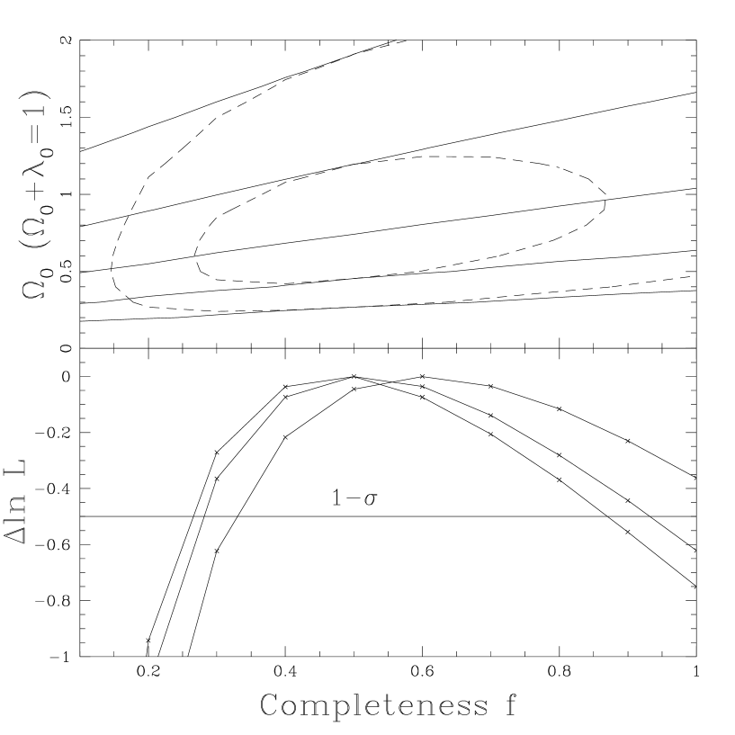
Figure 8: Completeness Estimates. The bottom panel shows the maximum likelihood as a function of the fractional completeness of the quasar lens sample $f$. We can equivalently view $f$ as the fraction of early-type galaxies made opaque in the optical by extinction. The top frame shows the limits on $\Omega_{0}$ for flat cosmologies and completeness model C. Notation is the same as for Figure 7.

The addition of the constraint that the total comoving galaxy density is far more certain than its division into spiral and early-type galaxies increases the importance of the spirals in determining the cosmological limits. Previously, as we increased the cosmological constant, the model would compensate by reducing the comoving densities of both galaxy types. Now, as the density of the early-type galaxies decreases, the density of spirals increases because of the constraint on the total galaxy density. The extra optical depth of the spirals limits the effectiveness of changes in the luminosity function in compensating for the change in cosmology and strengthens the cosmological limits. The quasars lensed by spirals are more affected by both extinction (Kochanek 1996b; Perna, Loeb & Bartelmann 1997) and biases against including lensed quasars in quasar catalogs (Kochanek 1991) than those lensed by early-type galaxies; therefore, we computed the optical sample both with and without spiral galaxies. We find better consistency with the radio sample (at the 1$-\sigma$ level) if we exclude spiral lenses from the optical sample; we use such a model as our standard.

Even after excluding quasars lensed by spirals, the optical sample prefers cosmological models with lower optical depths than the radio sample. Equivalently, this sample may be more affected by incompleteness due to extinction in the lens galaxies or systematic effects of surveys for quasars on the lensed quasars. To estimate the possible level of extinction we computed the quasar lensing probabilities assuming that each lens is intrinsically $\langle\Delta m\rangle$ mag brighter than observed, where $\langle\Delta m\rangle$ is the mean magnitude change due to extinction. The shift $\langle\Delta m\rangle$ can also represent errors in the magnitude of the break in the quasar luminosity function or offsets between the magnitude scale used for the individual quasars and the quasar luminosity function. Figure 7 shows the likelihood as a function of $\langle\Delta m\rangle$ and the corrected cosmological limits. The best fit value for the conservative completeness model C is $\langle\Delta m\rangle=0.58\pm 0.45$, and zero extinction is ruled out at slightly better than 1$-\sigma$ in the likelihood ratio. For the best fit model we still find $\Omega_{0}>0.26$ at 2$-\sigma$. For completeness model A we find $\langle\Delta m\rangle=0.53\pm 0.45$ and $\Omega_{0}>0.27$, and for model B we find $\langle\Delta m\rangle=0.40\pm 0.45$ and $\Omega_{0}>0.33$. A negative $\Delta m$ is possible; it corresponds either to an error in the quasar LF break magnitude or incompleteness in the radio sample. For the Seaton (1979) model of the UV extinction curve and a typical lens redshift of $0.5$, $\langle\Delta m\rangle\simeq 6E(B-V)$; thus, the magnitude changes correspond to $E(B-V)\simeq 0.1$. We can also give the quasars a relative completeness of $f$ compared to the radio sources by rescaling the comoving density of galaxies lensing the quasars to a fraction $f$ of the true density. The model mimics both incompleteness of the lensed quasar samples due to biases in quasar searches against lensed quasars (possibly a 10–20% effect, Kochanek 1991), and a bimodal extinction distribution for galaxies with fraction $f$ transparent and fraction $1-f$ opaque. As illustrated in Figure 8, the best fit for completeness model C is $f=0.48$ with a 1$-\sigma$ range from $0.26<f<0.87$ and a 2$-\sigma$ bound of $\Omega_{0}>0.25$ in flat models. For Model A the best fit is $f=0.52$ ($0.28<f<0.93$) and for Model B the best fit is $f=0.61$ ($0.33<f\lesssim 1.0$). In both models there is evidence that the quasar lens sample is significantly incomplete, although the significance of the result is weak because of the large Poisson uncertainties in the two samples.

4 Conclusions

We are conducting a redshift survey of 177 flat-spectrum radio sources in the flux range from 50 to 250 mJy; we have measured 124 redshifts that enabled us to estimate the cosmological model from the statistics of the 6 lensed radio sources found in the JVAS survey (Patnaik et al. 1992a; Patnaik 1994; King et al. 1996; Browne et al. 1997) of 2500 flat-spectrum sources brighter than 200 mJy. The mean redshifts of the sources are $\langle z\rangle\simeq 1.2$; they show little variation with the radio flux below 500 mJy. A rapidly increasing fraction of the sources consists of radio galaxies rather than radio quasars, rising from $\sim$ 10% of sources brighter than 1 Jy to $\sim$ 50% of sources at 100 mJy. The rapid change in the source population from blue quasars to red galaxies means that radio lenses will typically be redder than radio sources of the same flux and that many lensed flat-spectrum radio sources will show extended lensed optical emission, as already observed in MG 0414+0534 (Angonin-Willaime et al. (1994); Lawrence et al. (1995); Falco et al. (1997)) and CLASS 1608+656 (Myers et al. (1995); Jackson et al. 1997).

The cosmological limits from the radio-selected sample are statistically consistent with those derived from lensed quasars (see Maoz & Rix 1993, Kochanek 1993, 1996a). The 2$-\sigma$ limits on the cosmological constant in flat models for the radio, optical, and joint samples using the most conservative model for the completeness of our redshift surveys and excluding quasars lensed by spirals are $\Omega_{0}>0.27$, $0.31$, and $0.38$ respectively. The 1$-\sigma$ limits are $0.47<\Omega_{0}<1.38$, $0.65<\Omega_{0}$, and $0.64<\Omega_{0}<1.66$. The small numbers of lenses and the slow decline of the optical depth for large $\Omega_{0}$ mean that we find no 2$-\sigma$ upper bound for all three models and no 1$-\sigma$ upper bound for the optical sample up to the limit of $\Omega_{0}<2$. The weaker variation of the optical depth for cosmologies without a cosmological constant gives us only 1$-\sigma$ lower bounds on $\Omega_{0}$ of 0.24, 0.30, and 0.51 respectively. For comparison, Perlmutter et al. (1997) formally obtained 1$-\sigma$ limits of $0.66<\Omega_{0}<1.28$ for flat models and $0.28<\Omega_{0}<1.57$ for $\lambda_{0}=0$ models using Type Ia supernovae. Their formal statistical limits did not include several of the expected systematic uncertainties (e.g., extinction, K-correction models, Malmquist biases) which can produce additional uncertainties of $\Delta\Omega_{0}\sim 0.2$ (Perlmutter et al. 1997). The essentially perfect statistical consistency of these two radically different methods and the internal consistency of the radio and optical lens methods for determining the global cosmological model is a very reassuring check that neither approach has missed a catastrophic systematic error.

The agreement between the optical and radio samples is better (by about 1$-\sigma$) if there is no spiral galaxy contribution to the lensed quasars; we adopted a spiral-free model as our standard. The optically selected samples are biased against the inclusion of spirals both because of the higher extinction expected for spirals compared to early-types and because optical surveys to find quasars are more likely to exclude lenses produced by spirals than those produced by early-types. Kochanek (1991) noted that color and spectral selection methods for finding quasars were intrinsically biased against including lensed quasars, but that for bright quasars ($m<19$) lensed by early-type galaxies the effects were small ($\lesssim 10$%). However, a spiral galaxy lens is 1 to 2 mag brighter than an early-type lens for the same image separation and more easily masks the presence of the lensed quasar images. Where we have optical images of the quasar lens galaxies, they are all consistent with early-type galaxies, while a few of the radio lenses appear to be spirals (see Keeton, Kochanek & Falco 1997 for a summary). It is thus plausible that the combined effects of extinction and the optical quasar survey biases have eliminated most spiral lenses from the quasar lens sample.

Even after eliminating the spiral galaxies from the quasar analysis, the best fit optical depth implied by the quasars is less than that implied by the radio sources. We may be overestimating the radio optical depth by including the two lenses with significant extended radio structure (B 1938+666 and B 2114+022), because extended sources can have significantly higher probabilities of being lensed (Kochanek & Lawrence 1990). Although only 5% of the JVAS sources are extended or multi-component (Patnaik et al. 1992b), $15-30$% of the lensed sources are extended or multi-component depending on whether B 2114+022 is 2 images of a double source or 4 images of a single source (see Browne et al. 1997). Alternatively, we may be underestimating the quasar optical depth by neglecting either extinction in early-type galaxies (Kochanek 1991, 1996a; Tomita 1995; Malhotra et al. (1996)) or the biases in quasar surveys against lensed quasars (Kochanek 1991). When we fitted models where the mean lensed quasar is $\langle\Delta m\rangle$ mag fainter due to extinction, we found $\langle\Delta m\rangle=0.58\pm 0.45$; when we fitted models in which a fraction $f$ of quasar lenses are lost due to survey biases or opaque galaxies we found $f=0.48_{-0.22}^{+0.39}$. In both cases the model with no selection effect is ruled out at slightly over 1$-\sigma$. Even so, the limits on the cosmological constant remain reasonably robust, with $\Omega_{0}>0.26$ at 2$-\sigma$ in flat models. A mean magnitude change of $\langle\Delta m\rangle\sim 0.6$ corresponds to $E(B-V)\simeq 0.1$ in the lens galaxy, a $B-V$ color change of about $0.1$ mag and a $B-K$ color change of approximately $0.5$ mag.

Malhotra et al. (1996) have argued for a far larger effect from dust on the optically selected samples, largely by comparing the colors of radio selected lenses to the colors of optically selected lenses. They advocate a mean magnitude change of $\langle\Delta m\rangle\sim 2\pm 1$, or about 4 times our estimate. We believe Malhotra et al. (1996) were comparing the colors of intrinsically different populations, leading them to overestimate the effects of extinction. We see the population shift in our redshift survey with the rapidly rising fraction of (early-type) galaxies at fainter radio fluxes, and we see the population shift in the lensed sources by the frequent appearance of extended lensed optical emission (MG 0414+0534, CLASS 1608+656) and the frequent lack of the broad emission lines characteristic of quasars. Most of the observed lenses where there is a consensus for extinction of the source by the lens galaxy are clearly spiral lenses either because we directly observe the spiral structure (2237+0305, Nadeau et al. 1991) or from the presence of atomic and molecular gas (B 0218+357 and PKS 1830–210, Carilli, Rupen, & Yanny 1993; Wicklind & Combes 1996; Lovell et al. 1996). The exception is MG 0414+0534 (Lawrence et al. (1995)), where the lens galaxy itself is far redder than any passively evolving early-type galaxy or any other lens galaxy (Falco et al. 1997; Keeton, Kochanek & Falco 1997). We also cannot use MG 0414+0534 to make simple inferences about lensed quasars because the very presence of extended lensed optical emission means that the source is very different from a bright optical quasar. A likely counter hypothesis to that of Malhotra et al. (1996) is that all extremely red lensed sources will turn out to have extended lensed optical emission in deep HST images.

The general agreement of the radio and optical samples does not eliminate the question of common systematic dependencies. The most important problem is the continuing uncertainty in the galaxy luminosity function, particularly when divided by type; the statistical uncertainties in the present models are roughly equally due to the Poisson uncertainties from the numbers of lenses and the uncertainties in the local comoving density of early-type galaxies. The models do not include any evolution in the galaxy populations, although models of lensing with galaxy evolution (Mao 1991; Mao & Kochanek 1994; Rix et al. 1994) demonstrated that lens statistics are considerably less sensitive to galaxy evolution than one might naively expect. Most plausible merger models conserve the optical depth while changing the separation distribution. Moreover, since the mean lens redshift is usually less than $z=1$, redshift surveys have already confirmed that the early-type population that dominates gravitational lensing shows little evolution (e.g. Lilly et al. 1995). Nonetheless, evolution is a significant systematic question that we should address in greater detail.

Our ability to expand the cosmological conclusions is largely restricted by the need for additional redshift data. The incompleteness of our redshift survey leads to uncertainties of $\Delta\Omega_{0}\simeq 0.1$ in the cosmological model, and despite our survey, we still cannot include the majority of the known radio lenses found in systematic surveys in our analysis for lack of data on the luminosity function. Interpreting the CLASS survey (5 lenses so far) requires that the flat-spectrum redshift distribution be extended to $\sim 5$ mJy, and interpreting the MG Survey (5 lenses so far) requires that the steep-spectrum redshift distribution be extended to $\sim 100$ mJy. The lensing optical depth varies strongly along lines of constant $\Omega_{0}+\lambda_{0}$, and rather weakly in the orthogonal direction, leading to the degenerate likelihood contours in the $\Omega_{0}$-$\lambda_{0}$ plane shown in Figure 5. One way to break the degeneracy, and also to strengthen the overall limits, is to use the distribution of lens galaxy redshifts compared to source redshifts (Kochanek 1992), because the mean lens redshift has a different dependence on $\Omega_{0}$ and $\lambda_{0}$ than the optical depth (Kochanek 1993). Unfortunately, both the source and lens redshifts are known for only a small fraction of the lenses, and the corrections for incompleteness when using the lens redshifts are both important and difficult to model (Helbig & Kayser (1996); Kochanek 1996a).

Table 2: Sample 1 (JVAS 200–250 mJy)

Object	$\alpha$ (B1950)	$\delta$ (B1950)	$I$	$\sigma_{I}$	$z$	$\sigma_{z}$	type               detected lines
0902+468	09 02 52.68	46 48 21.71	14.8	0.2	0.0848	0.0005	E	(HK, H$\delta$, G, Mg, CaFe, Na), H$\alpha$, OIII
0903+669	09 03 01.85	66 56 51.58	18.9	0.2
0905+420	09 05 20.99	42 02 56.14	18.2	0.1	0.7325	0.0008	Q	CIII$\left.\right]$, MgII, H$\gamma$, H$\beta$
0920+416	09 20 19.92	41 38 20.60	18.0	0.1	0.028	0.001	L	(HK, H$\beta$, Mg, CaFe, Na), H$\alpha$, OIII
0924+732	09 24 51.83	73 17 12.42	18.6	0.1			D
0927+469	09 27 17.71	46 57 20.96	16.8	0.2	2.032	0.001	Q	Ly$\alpha$, SiIV, CIV, CIII$\left.\right]$
0927+586	09 27 10.76	58 36 35.55	17.1	0.1	1.9645	0.0009	Q	Ly$\alpha$, SiIV, CIV, HeII, CIII$\left.\right]$
0939+620	09 39 29.44	62 04 17.76	18.0	0.2	0.7533	0.0005	Q	MgII, NeV
0951+422	09 51 06.97	42 15 20.74	19.3	0.1	1.783	0.004	Q	SiIV, CIV, CIII$\left.\right]$, MgII
0955+509	09 55 22.22	50 54 18.83	17.7	0.2	1.154	0.002	Q	CIV, CIII$\left.\right]$, CII, MgII, HeI
1010+495	10 10 20.75	49 33 33.83	18.5	0.1	2.201	0.002	Q	Ly$\alpha$, CIV, CIII$\left.\right]$
1023+747	10 23 13.02	74 43 44.02	17.5	0.2	0.879	0.002	Q	MgII, OIII, OIV
1027+749†	10 27 13.30	74 57 23.11	15.2	0.2	0.123	0.001	E
1028+564	10 28 50.61	56 26 23.42	21.5	0.5			D
1101+609	11 01 50.75	60 55 07.10	18.9	0.2	1.363	0.003	Q	CIV, CIII$\left.\right]$, MgII
1109+350	11 09 55.21	35 02 58.82	19.1	0.2	1.9495	0.0003	Q	Ly$\alpha$, CIV, CIII$\left.\right]$
1116+603†	11 16 19.23	60 21 22.49	17.5	0.2	2.638		Q
1117+543	11 17 33.00	54 20 53.33	18.8	0.2	0.924	0.001	Q	CIII$\left.\right]$, MgII, OIIIa, NeV, H$\gamma$
1131+730	11 31 11.77	73 05 55.21	18.2	0.2	1.571	0.002	Q	SiIV, CIV, HeII, CIII$\left.\right]$, MgII
1147+438	11 47 39.81	43 48 47.00	18.8	0.1	3.037	0.008	N	Ly$\alpha$, CIV, CIII$\left.\right]$
1151+598	11 51 24.00	59 51 35.93	19.9	0.2	0.871	0.002	Q	CIII$\left.\right]$, MgII, H$\gamma$
1200+468	12 00 58.77	46 49 37.77	21.4	0.2
1200+608	12 00 30.71	60 48 01.36	14.4	0.1	0.0656	0.0002	E	HK, H$\delta$, Mg, CaFe, Na
1204+399	12 04 04.63	39 57 45.72	18.2	0.2	1.5134	0.0009	Q	CIV, CIII$\left.\right]$, CII, MgII
1231+507	12 31 27.08	50 42 54.89	16.7	0.1	0.2075	0.0005	E	HK, G, Mg, CaFe Na
1234+396	12 34 26.25	39 36 57.85	19.0	0.2			D
1238+702	12 38 32.70	70 14 57.98	16.6	0.1	1.4706	0.0005	Q	CIV, CIII$\left.\right]$, MgII
1239+606	12 39 16.55	60 37 08.06	16.8	0.1	1.457	0.005	N	SiIV, CIV, NIII, CIII$\left.\right]$
1245+676	12 45 32.18	67 39 38.12	16.9	0.2	0.1073	0.0002	E	(HK, H$\delta$, G, H$\beta$, Mg, CaFe, Na)
1245+716	12 45 15.69	71 40 41.97	20.8	0.3			D
1300+485	13 00 03.36	48 35 24.34	16.1	0.2	0.873	0.001	Q	CIII$\left.\right]$, CII, MgII, HeI
1300+693	13 00 50.97	69 18 57.72	17.1	0.2	0.5677	0.0003	L	CII, NeV, OII, HeI, H$\gamma$, OIII
1302+356	13 02 15.38	35 39 57.94	21.7	0.3
1310+487	13 10 32.94	48 44 24.63	19.3	0.2	(0.313)	0.003	L	OIII, NeV, H$\gamma$, H$\beta$
1318+508	13 18 36.32	50 51 50.13	21.2	0.7			D
1327+504	13 27 02.23	50 24 55.57	18.1	0.2	2.654	0.001	Q	OVI, SIV, Ly$\alpha$, SiIV, CIV
1328+523	13 28 41.69	52 17 41.92	19.3	0.2			D
1339+696	13 39 29.98	69 38 30.80	18.7	0.2	2.255	0.003	B	Ly$\alpha$, CIV, CIII$\left.\right]$
1341+691	13 41 42.19	69 10 21.11	17.3	0.2	1.417	0.002	Q	CIV, CIII$\left.\right]$, CII, MgII
1349+618	13 49 01.61	61 47 37.87	20.7	0.4	1.834	0.002	Q	CIV, NIII, CIII$\left.\right]$, NeIV
1409+595	14 09 49.22	59 31 08.20	20.1	0.2	1.725	0.009	Q	CIV, CIII$\left.\right]$, MgII
1412+461	14 12 19.18	46 08 46.22	19.9	0.2	0.186	0.002	E	(HK, H$\delta$, CaFe, Na)
1418+375	14 17 55.81	37 35 18.25	17.9	0.1	0.969	0.002	B	NIII, CIII$\left.\right]$, MgII
1419+469	14 19 30.38	46 59 27.87	16.2	0.2	1.665	0.003	Q	SiIV, CIV, CIII$\left.\right]$, MgII
1421+511†	14 21 28.55	51 09 12.34	15.0	0.2	0.274	0.002	Q
1427+634	14 27 52.03	63 29 23.84	20.9	0.2	1.561	0.001	Q	CIV, HeII, CIII$\left.\right]$, CII, MgII
1438+501	14 38 04.29	50 10 56.24	17.7	0.2	0.174	0.002	E	(HK, H$\delta$, G, Mg, H$\beta$, CaFe)
1447+536	14 47 26.02	53 38 33.49	22.1	0.5
1450+455†	14 50 37.18	45 34 38.12	16.0	0.2	0.469		E
1454+447	14 54 06.02	44 43 41.66	17.8	0.2
1533+487	15 33 42.16	48 46 54.20	16.2	0.2	2.563	0.002	N	Ly$\alpha$, CIV, CIII$\left.\right]$
1556+745	15 56 54.94	74 29 32.56	19.3	0.2	1.667	0.001	Q	CIV, HeII, CIII$\left.\right]$, MgII
1557+565	15 57 41.57	56 33 41.87	16.0	0.1	0.30	0.03	E	(HK, H$\delta$, G)
1558+595	15 58 05.76	59 32 48.42	15.0	0.2	0.0602	0.0001	E	(HK, H$\delta$, G, H$\beta$, Mg, CaFe, Na)
1603+573	16 03 34.72	57 22 42.20	16.3	0.2	0.720	0.001	Q	CIII$\left.\right]$, MgII, NeV, H$\gamma$, H$\beta$
1611+425	16 11 25.57	42 30 52.93	20.3	0.4
1627+476	16 27 11.18	47 40 42.41	18.4	0.2	1.629	0.001	Q	SiIV, CIV, HeII, CIII$\left.\right]$, CII, MgII
1646+411	16 46 50.96	41 09 16.65	20.0	0.2	0.8508	0.0003	Q	CIII$\left.\right]$, MgII, H$\gamma$
1646+499	16 46 16.48	49 55 14.75	14.1	0.2	0.0475	0.0001	L	(HK, G, Mg, CaFe, Na), H$\alpha$, OIII
1650+581	16 50 31.80	58 10 39.84	22.5	1.0
1655+534	16 55 32.40	53 26 24.60	16.9	0.2	1.553	0.002	Q	CIV, CIII$\left.\right]$, MgII
1704+512	17 04 13.38	51 13 34.34	16.7	0.2	0.5303	0.0003	Q	MgII, NeV, HeI, OIII
1712+493	17 12 17.48	49 19 56.91	19.3	0.2	1.552	0.002	Q	CIV, HeII, CIII$\left.\right]$, MgII
1738+451	17 38 39.49	45 08 20.42	15.7	0.2	2.788	0.008	N	Ly$\alpha$, CIV, CIII$\left.\right]$
1742+378	17 42 05.62	37 49 08.35	16.4	0.2	1.9578	0.0005	Q	Ly$\alpha$, SiIV, CIV, HeII, CIII$\left.\right]$
1745+643†	17 45 51.98	64 22 50.89	20.8	0.3	1.228		E
1750+509	17 50 21.11	50 56 17.43	16.5	0.2	0.3284	0.0004	L	(HK, H$\delta$, G, Mg, CaFe), Mg, OII, H$\gamma$, OIII
1752+356	17 52 27.92	35 41 17.64	16.8	0.2	2.207	0.002	Q	Ly$\alpha$, CIV, CIII$\left.\right]$
1755+626	17 55 23.68	62 37 03.36	15.1	0.4	0.0276	0.0001	E	(HK, H$\beta$, Mg, CaFe, Na)

Note. — A $\dagger$ indicates a previously known source as per NED, for which we did not obtain spectra; HK and G are the CaII H&K lines and G bands, respectively; parentheses surrounding a list of lines indicate absorption; parentheses surrounding a redshift indicate a marginal measurement; D, E, L, Q, B, N and b indicate respectively a detected object, an early-type galaxy, a late-type galaxy, a quasar, a quasar with broad absorption lines, a quasar with narrow absorption lines and a BL Lac object.

Table 3: Sample 2 (MG 100–200 mJy)

Object	$\alpha$ (B1950)	$\delta$ (B1950)	$I$	$\sigma_{I}$	$z$	$\sigma_{z}$	type               detected lines
MGC0001+2113	23 58 58.58	56 54.04	17.7	0.1	1.106	0.002	Q	CIII$\left.\right]$, NeV, HeI
MGC0034+3712	00 32 14.32	55 53.66	18.9	0.2	1.390	0.002	Q	CIV, CIII$\left.\right]$, MgII
MGC0037+2613	00 34 40.35	56 43.50			0.1477	0.0002	E	(HK, G, H$\beta$, Mg)
MGC0042+2739	00 39 55.71	23 22.41
MGC0046+2249	00 43 41.10	33 20.37
MGC0046+2456	00 43 28.10	40 09.40	17.1	0.2	0.7467	0.0004	Q	NeIV, MgII, HeI
MGC0054+2549	00 51 54.96	33 49.06
MGC0054+3842	00 51 27.85	25 58.52
MGB1606+2031	16 03 54.30	40 12.40
MGB1634+1946	16 32 34.50	53 14.76	17.9	0.2	0.792	0.003	Q	CIII$\left.\right]$, CII, MgII, HeI
MGB1655+1949	16 53 32.99	53 29.07	16.6	0.2	3.260	0.003	N	Ly$\beta$, Ly$\alpha$, SiIV, CIV
MGB1705+2215	17 03 22.21	20 08.25			0.04977	0.00008	E	(HK, G, H$\beta$, Mg, CaFe, Na)
MGB1715+3619	17 13 22.85	23 08.90	18.4	0.2	0.5549	0.0003	Q	MgII, HeI, H$\beta$, OIII
MGB1720+2334	17 18 05.64	38 29.12	17.4	0.2	1.852	0.003	Q	Ly$\alpha$, SiIV, CIV, CIII$\left.\right]$, MgII
MGB1728+1931	17 26 44.62	33 31.38			0.1756	0.0003	E	(HK, G, H$\beta$, Mg, CaFe, Na)
MGB1745+2252	17 42 59.09	53 57.86	17.5	0.2	1.8838	0.0007	Q	Ly$\alpha$, SiIV, CIV, HeII, CIII$\left.\right]$
MGB1747+2323	17 45 45.21	25 37.51	17.1	0.1	2.203	0.002	N	Ly$\beta$, Ly$\alpha$, SiIV, CIV
MGB1807+3107	18 05 38.33	05 52.75	18.3	0.2	0.5373	0.0004	N	MgII, NeV, OIII
MGB1813+3144†	18 11 42.73	43 22.31	16.3	0.1	0.117		b
MGB1834+2051	18 32 03.59	49 16.53	16.8	0.2			D
MGB1835+2506	18 33 55.57	04 13.20			1.9728	0.0009	B	CIV, CIII$\left.\right]$
MGB1843+3150	18 41 10.08	47 23.59	15.9	0.1	0.4477	0.0003	Q	MgII, NeV, HeI, H$\gamma$, H$\beta$
MGB1843+3225	18 41 37.21	22 22.47	16.8	0.3			D
MGB1846+2036	18 43 55.22	32 54.81	16.9	0.1			D
MGB1853+2344	18 51 22.48	40 48.28	14.1	0.2	1.0311	0.0008	Q	CIII$\left.\right]$, MgII
MGC2036+2227	20 34 44.58	17 29.07	16.4	0.1	2.567	0.002	Q	Ly$\alpha$, SiIV, CIV, CIII$\left.\right]$
MGB2043+2256	20 41 40.27	46 26.50	16.7	0.1	1.0810	0.0003	Q	CIII$\left.\right]$, MgII
MGB2051+1950	20 48 56.61	38 48.99	16.6	0.1	2.365	0.002	Q	Ly$\alpha$, SiIV, CIV, CIII$\left.\right]$
MGC2054+2407	20 52 17.47	56 05.77	16.5	0.2	1.3774	0.0005	Q	CIV, CIII$\left.\right]$, MgII
MGC2100+2058	20 57 49.45	47 34.81	17.6	0.1	(0.19)	0.04	E	HK
MGC2100+2346	20 57 51.93	35 17.88	17.0	0.2	1.124	0.001	Q	CIV, HeII, CIII$\left.\right]$, MgII
MGC2100+2615	20 58 28.63	03 49.70					D
MGC2105+2920	21 03 35.78	08 49.82	18.6	0.1	1.347	0.002	Q	CIV, CIII$\left.\right]$, MgII
MGC2106+2135	21 03 55.28	23 31.85	17.8	0.1	0.6469	0.0008	Q	MgII, OII, OIII
MGC2109+2154	21 06 53.16	42 50.03	17.6	0.1	2.344	0.002	N	Ly$\alpha$, CIV, CIII$\left.\right]$
MGC2109+2211	21 07 40.17	00 00.30	18.4	0.1	2.281	0.002	Q	Ly$\alpha$, CIV, CIII$\left.\right]$
MGC2116+3016	21 13 59.43	04 05.38	17.3	0.2	2.080	0.003	N	Ly$\alpha$, SiIV, CIV, HeII, CIII$\left.\right]$
MGC2118+2006	21 16 08.43	54 54.12
MGC2125+2441	21 23 11.64	29 00.28
MGC2130+3332	21 28 22.92	19 35.42	17.9	0.2	1.473	0.006	Q	CIV, CIII$\left.\right]$, MgII
MGC2137+2357	21 34 49.60	43 31.15	17.1	0.2	0.6044	0.0007	Q	MgII, NeV, HeI, H$\gamma$, H$\beta$, OIII
MGC2153+2351	21 50 45.69	37 48.69
MGC2203+3712	22 01 08.58	56 45.03	14.5	0.2	1.817	0.005	N	Ly$\alpha$, CIV, MgII
MGC2213+2558	22 11 27.17	43 30.11	15.0	0.3	0.0940	0.0002	E	(HK, H$\delta$, G, H$\beta$, Mg, CaFe, Na)
MGC2214+3550	22 12 44.73	36 29.15	18.2	0.2	0.877	0.003	Q	CIII$\left.\right]$, CII, MgII
MGC2214+3739	22 11 55.07	24 14.24
MGC2223+2439	22 20 47.66	24 00.50	17.7	0.1	1.490	0.004	Q	SiIV, CIV, HeII, CIII$\left.\right]$, CII, MgII
MGC2227+3716	22 25 04.20	59 59.08	17.4	0.2	0.975	0.003	N	HeII, CIII$\left.\right]$, MgII, H$\gamma$
MGC2229+3057	22 27 15.93	41 48.78			0.3196	0.0004	L	NeV, HeI, H$\gamma$, H$\beta$, OIII
MGC2230+2752	22 27 55.30	38 18.77
MGC2250+3825	22 47 48.11	08 42.70			0.1187	0.0003	E	(HK, G, H$\beta$, Mg, CaFe, Na)
MGC2251+2217	22 49 27.88	01 40.50	20.2	0.2	3.668	0.003	N	SIV, Ly$\alpha$, CII, CIV
MGC2254+2058	22 52 27.05	42 36.60			0.0635	0.0002	E	(HK, H$\delta$, G, H$\beta$, Mg, CaFe, Na)
MGC2257+3706	22 55 15.49	50 26.43
MGC2301+3512	22 58 52.85	56 52.64			0.1357	0.0005	E	(HK, G, Mg, CaFe, Na), H$\alpha$, OIII
MGC2308+2008	23 05 43.49	52 26.67			0.2342	0.0007	L	MgII, H$\beta$, OIII, H$\alpha$
MGC2309+3726	23 06 51.15	09 53.28	18.3	0.2			D
MGC2315+3727	23 12 44.93	10 32.86
MGC2318+2404	23 16 05.73	48 14.79	17.2	0.1			D
MGC2344+3433	23 42 20.80	17 09.05	17.8	0.2	3.053	0.007	B	SVI, Ly$\beta$, Ly$\alpha$, CIV, CIII$\left.\right]$
MGC2348+3539	23 46 27.36	23 19.46
MGC2350+2331	23 47 43.12	15 19.61			1.693	0.001	Q	Ly$\alpha$, SiIV, CIV, HeII, CIII$\left.\right]$, MgII
MGC2356+3840	23 54 26.73	23 33.25	18.5	0.2	0.2281	0.0003	E	(HK, G, Mg, Na)

Note. — See Table 2 for comments and definitions of object types.

Table 4: Sample 3 (MG 50–100 mJy)

Object	$\alpha$ (B1950)	$\delta$ (B1950)	$I$	$\sigma_{I}$	$z$	$\sigma_{z}$	type               detected lines
MG0803+3055	08 00 24.04	31 05 04.57	19.6	0.2
MG0809+3122	08 06 05.02	31 31 12.00	15.7	0.1	0.220	0.001	b	(HK, G, Mg, Na)
MG0814+2809	08 11 55.85	28 18 47.00	20.5	0.2	(0.138)	0.006	L	(HK, H$\delta$, Na), OIII, H$\alpha$
MG0828+2919	08 25 05.42	29 30 17.01	18.5	0.1	2.322	0.005	Q	OVI, Ly$\alpha$, CIV, MgVII
MG0854+3009	08 51 31.15	30 21 24.85	21.6	0.3			D
MG0909+2911	09 06 16.86	29 23 40.33	20.2	0.2			D
MG0920+2755	09 17 30.79	28 08 38.00	23.1	1.0			D
MG0923+3059	09 20 07.97	31 12 18.00	17.2	0.1	0.6292	0.0006	Q	MgVII, MgII, NeV, HeI, H$\gamma$, H$\beta$
MG0926+2758	09 23 49.16	28 11 23.00
MG0932+2837	09 29 18.29	28 50 47.00	17.6	0.1	0.3033	0.0002	E	(HK, H$\delta$, G, H$\beta$, Mg, CaFe, Na)
MG0933+2844	09 30 41.39	28 58 52.00	18.3	0.2	3.428	0.002	N	Ly$\beta$, Ly$\alpha$, SiIV, CIV
MG0940+3015	09 37 22.49	30 28 47.00	17.8	0.1	1.594	0.002	Q	SiIV, CIV, HeII, CIII$\left.\right]$, CII, MgII
MG1013+3042	10 10 15.13	30 58 25.00	18.4	0.1
MG1019+3037	10 16 29.21	30 52 45.00	20.3	0.2	1.342	0.002	Q	CIV, HeII, CIII$\left.\right]$, MgVII, MgII
MG1023+2856	10 20 34.89	29 12 02.00	17.3	0.1
MG1028+3107	10 25 27.83	31 22 53.99	17.6	0.1	0.2403	0.0005	E	(HK, G, Mg, CaFe, Na), MgII, H$\alpha$
MG1044+2958	10 41 19.77	30 14 46.00	18.0	0.1	2.981	0.001	Q	OVI, SIV, Ly$\alpha$, SiIV, CIV
MG1045+3143	10 42 36.19	31 58 18.00	18.5	0.2	3.230	0.005	N	SIV, OVI, Ly$\alpha$, SiIV, CIV
MG1106+3000	11 03 41.30	30 16 58.00
MG1111+2841†	11 08 31.45	28 58 05.00			0.02937	0.00003	E
MG1112+2844	11 10 05.92	29 00 03.85
MG1137+2935	11 34 43.15	29 52 15.00	17.7	0.2	2.644	0.001	N	OVI, Ly$\alpha$, SiIV, CIV, HeII, CIII$\left.\right]$
MG1142+2855	11 40 17.63	29 11 27.00			0.0974	0.0002	E	(HK, H$\delta$, G, H$\beta$, Mg, CaFe, Na)
MG1145+2800	11 43 11.88	28 17 56.00	19.7	0.1
MG1146+2845	11 44 11.73	29 01 22.00
MG1202+2756†	12 00 00.50	28 13 07.00			0.672		Q
MG1213+2812	12 10 57.91	28 28 31.00
MG1215+2750	12 13 18.26	28 06 16.00	16.6	0.2	0.1034	0.0001	E	(HK, G, H$\beta$, Mg, CaFe, Na)
MG1301+2822†	12 58 55.76	28 37 44.00			1.373		Q
MG1310+2925†	13 07 43.24	29 42 15.00	18.0	0.2	1.21		Q
MG1312+3113	13 10 27.54	31 28 53.00	16.6	0.1	1.0533	0.0009	Q	CIII$\left.\right]$, MgII, NeV
MG1334+3043	13 32 04.52	30 59 32.00	15.4	0.1	1.352	0.001	N	SiIV, CIV, NIII, CIII$\left.\right]$, MgII
MG1340+3009	13 38 24.62	30 23 43.00	17.4	0.1
MG1342+2828†	13 40 36.25	28 43 10.00			1.037		Q
MG1346+2900	13 44 20.21	29 15 40.00
MG1347+2836‡	13 45 34.25	28 51 25.00	13.5	0.1			D
MG1353+2933	13 51 40.75	29 47 50.00	20.2	0.2			D
MG1354+3139†	13 51 51.20	31 53 45.00			1.326		Q
MG1355+3023†	13 53 26.22	30 38 51.00			1.018		Q
MG1356+2918	13 54 37.00	29 32 55.00	18.7	0.1	3.244	0.005	N	Ly$\alpha$, SiIV, CIV
MG1400+2918	13 57 53.82	29 32 57.00
MG1406+2930	14 03 56.65	29 45 58.00
MG1415+2823	14 13 23.64	28 37 14.00	16.6	0.1	0.2243	0.0003	E	(HK, G, H$\beta$, Mg, Na)
MG1437+3119†	14 35 31.49	31 31 57.00			1.366		Q
MG1438+3001	14 35 49.42	30 15 03.00	16.9	0.2	0.2316	0.0003	E	(G, H$\beta$, Mg, CaFe, Na), MgII, NeV

Note. — See Table 2 for comments and definitions of object types. A $\ddagger$ indicates likely contamination of the magnitude by a foreground star.

Table 5: Serendipitous Objects in JVAS (200-250 mJy)

Object	$\alpha$ (B1950)	$\delta$ (B1950)	$z$	$\sigma_{z}$	type	lines
0707+424	07 10 44.3	42 20 55.0	1.1645	0.0003	Q	CIII$\left.\right]$, MgII
0718+374	07 22 01.6	37 22 28.6	1.629	0.001	Q	CIV, CIII$\left.\right]$, MgII
0806+350	08 09 38.9	34 55 37.3	0.0823	0.0002	L	(HK, G, H$\beta$, Mg, CaFe, Na), H$\alpha$
0932+367	09 35 31.8	36 33 17.6	2.852	0.003	Q	Ly$\alpha$, CIV, HeII, CIII$\left.\right]$
1035+430	10 38 18.2	42 44 42.8	0.3055	0.0002	L	(HK, H$\delta$, G), OII, H$\beta$, OIII

Note. — See Table 2 for comments and definitions of object types.

Table 6: Limits on Flat Cosmological Models

Model	$\ln L$	max	1-$\sigma$	2-$\sigma$
OPT	$-34.98$	$1.24$	$0.65<\Omega_{0}<\hphantom{1.60}$	$0.31<\Omega_{0}<\hphantom{1.60}$
OPT–S	$-35.17$	$1.59$	$0.94<\Omega_{0}<\hphantom{1.60}$	$0.55<\Omega_{0}<\hphantom{1.60}$
RAD–A	$-11.05$	$0.86$	$0.50<\Omega_{0}<1.47$	$0.29<\Omega_{0}<\hphantom{1.60}$
RAD–B	$-11.05$	$1.01$	$0.60<\Omega_{0}<1.69$	$0.36<\Omega_{0}<\hphantom{1.60}$
RAD–C	$-11.05$	$0.80$	$0.47<\Omega_{0}<1.38$	$0.27<\Omega_{0}<\hphantom{1.60}$
RAD–A+OPT	$-46.55$	$1.07$	$0.66<\Omega_{0}<1.71$	$0.39<\Omega_{0}<\hphantom{1.60}$
RAD–B+OPT	$-46.32$	$1.15$	$0.72<\Omega_{0}<1.81$	$0.44<\Omega_{0}<\hphantom{1.60}$
RAD–C+OPT	$-46.66$	$1.04$	$0.64<\Omega_{0}<1.66$	$0.38<\Omega_{0}<\hphantom{1.60}$
RAD–A+OPT–S	$-47.01$	$1.28$	$0.84<\Omega_{0}<1.95$	$0.55<\Omega_{0}<\hphantom{1.60}$
RAD–B+OPT–S	$-46.71$	$1.35$	$0.89<\Omega_{0}<\hphantom{1.60}$	$0.58<\Omega_{0}<\hphantom{1.60}$
RAD–C+OPT–S	$-47.15$	$1.26$	$0.82<\Omega_{0}<1.92$	$0.54<\Omega_{0}<\hphantom{1.60}$
RAD–C+OPT–a01	$-46.42$	$0.97$	$0.59<\Omega_{0}<1.56$	$0.35<\Omega_{0}<\hphantom{1.60}$
RAD–C+OPT–a02	$-46.22$	$0.91$	$0.56<\Omega_{0}<1.46$	$0.33<\Omega_{0}<\hphantom{1.60}$
RAD–C+OPT–a03	$-46.06$	$0.85$	$0.52<\Omega_{0}<1.37$	$0.30<\Omega_{0}<\hphantom{1.60}$
RAD–C+OPT–a04	$-45.95$	$0.80$	$0.49<\Omega_{0}<1.29$	$0.29<\Omega_{0}<\hphantom{1.60}$
RAD–C+OPT–a05	$-45.88$	$0.75$	$0.46<\Omega_{0}<1.21$	$0.27<\Omega_{0}<1.93$
RAD–C+OPT–a06	$-45.87$	$0.71$	$0.43<\Omega_{0}<1.15$	$0.26<\Omega_{0}<1.83$
RAD–C+OPT–a07	$-45.91$	$0.68$	$0.41<\Omega_{0}<1.09$	$0.24<\Omega_{0}<1.74$
RAD–C+OPT–a08	$-45.99$	$0.64$	$0.39<\Omega_{0}<1.03$	$0.23<\Omega_{0}<1.66$
RAD–C+OPT–a09	$-46.15$	$0.62$	$0.37<\Omega_{0}<0.99$	$0.22<\Omega_{0}<1.58$
RAD–C+OPT–a10	$-46.37$	$0.59$	$0.36<\Omega_{0}<0.95$	$0.20<\Omega_{0}<1.52$
RAD–C+OPT–f01	$-48.78$	$0.49$	$0.29<\Omega_{0}<0.79$	$0.18<\Omega_{0}<1.28$
RAD–C+OPT–f02	$-46.85$	$0.55$	$0.34<\Omega_{0}<0.89$	$0.19<\Omega_{0}<1.44$
RAD–C+OPT–f03	$-46.18$	$0.62$	$0.38<\Omega_{0}<1.00$	$0.22<\Omega_{0}<1.60$
RAD–C+OPT–f04	$-45.95$	$0.68$	$0.41<\Omega_{0}<1.10$	$0.25<\Omega_{0}<1.76$
RAD–C+OPT–f05	$-45.91$	$0.74$	$0.45<\Omega_{0}<1.19$	$0.27<\Omega_{0}<1.91$
RAD–C+OPT–f06	$-45.98$	$0.81$	$0.49<\Omega_{0}<1.29$	$0.29<\Omega_{0}<\hphantom{1.60}$
RAD–C+OPT–f07	$-46.11$	$0.86$	$0.53<\Omega_{0}<1.39$	$0.31<\Omega_{0}<\hphantom{1.60}$
RAD–C+OPT–f08	$-46.28$	$0.92$	$0.56<\Omega_{0}<1.48$	$0.33<\Omega_{0}<\hphantom{1.60}$
RAD–C+OPT–f09	$-46.46$	$0.98$	$0.60<\Omega_{0}<1.57$	$0.36<\Omega_{0}<\hphantom{1.60}$
Type Ia Supernova		$0.94$	$0.66<\Omega_{0}<1.28$	$0.51<\Omega_{0}<\hphantom{1.60}$

Note. — An empty entry means that the statistical limit was not reached at the edge of the range $0<\Omega_{0}<2$ and $-1<\lambda_{0}<1$. “RAD-A (B,C)” designates the radio data with completeness model A (B, C), “OPT” and “OPT-S” designate the optical data either with or without spiral galaxy lenses, $-axx$ indicates a mean magnitude change of $\langle\Delta m\rangle=xx$, and $-fxx$ indicates an optical completeness of $f=xx$. The Perlmutter et al. (1997) results for Type Ia supernovae are also shown, with a blank entry indicating that the limits was not given.

Table 7: Limits on $\lambda_{0}=0$ Cosmological Models

Model	$\ln L$	max	1-$\sigma$	90% confid   d
OPT	$-35.00$	$1.38$	$0.30<\Omega_{0}<\hphantom{1.60}$	$\hphantom{1.60}<\Omega_{0}<\hphantom{1.60}$
OPT–S	$-39.58$	$1.95$	$\hphantom{1.60}<\Omega_{0}<\hphantom{1.60}$	$\hphantom{1.60}<\Omega_{0}<\hphantom{1.60}$
RAD–A	$-11.06$	$1.12$	$0.32<\Omega_{0}<\hphantom{1.60}$	$\hphantom{1.60}<\Omega_{0}<\hphantom{1.60}$
RAD–B	$-10.97$	$1.45$	$0.49<\Omega_{0}<\hphantom{1.60}$	$0.13<\Omega_{0}<\hphantom{1.60}$
RAD–C	$-11.12$	$1.09$	$0.24<\Omega_{0}<\hphantom{1.60}$	$\hphantom{1.60}<\Omega_{0}<\hphantom{1.60}$
RAD–A+OPT	$-46.46$	$1.44$	$0.55<\Omega_{0}<\hphantom{1.60}$	$0.19<\Omega_{0}<\hphantom{1.60}$
RAD–B+OPT	$-46.21$	$1.53$	$0.65<\Omega_{0}<\hphantom{1.60}$	$0.27<\Omega_{0}<\hphantom{1.60}$
RAD–C+OPT	$-46.59$	$1.42$	$0.51<\Omega_{0}<\hphantom{1.60}$	$0.16<\Omega_{0}<\hphantom{1.60}$
RAD–A+OPT–S	$-46.82$	$1.77$	$0.88<\Omega_{0}<\hphantom{1.60}$	$0.46<\Omega_{0}<\hphantom{1.60}$
RAD–B+OPT–S	$-46.50$	$1.92$	$0.97<\Omega_{0}<\hphantom{1.60}$	$0.54<\Omega_{0}<\hphantom{1.60}$
RAD–C+OPT–S	$-46.97$	$1.74$	$0.84<\Omega_{0}<\hphantom{1.60}$	$0.43<\Omega_{0}<\hphantom{1.60}$
RAD–C+OPT–a01	$-46.38$	$1.14$	$0.43<\Omega_{0}<\hphantom{1.60}$	$0.11<\Omega_{0}<\hphantom{1.60}$
RAD–C+OPT–a02	$-46.21$	$1.11$	$0.36<\Omega_{0}<\hphantom{1.60}$	$0.06<\Omega_{0}<\hphantom{1.60}$
RAD–C+OPT–a03	$-46.11$	$1.07$	$0.29<\Omega_{0}<\hphantom{1.60}$	$0.01<\Omega_{0}<\hphantom{1.60}$
RAD–C+OPT–a04	$-46.02$	$0.80$	$0.22<\Omega_{0}<1.86$	$\hphantom{1.60}<\Omega_{0}<\hphantom{1.60}$
RAD–C+OPT–a05	$-45.99$	$0.77$	$0.17<\Omega_{0}<1.71$	$\hphantom{1.60}<\Omega_{0}<\hphantom{1.60}$
RAD–C+OPT–a06	$-46.03$	$0.72$	$0.12<\Omega_{0}<1.59$	$\hphantom{1.60}<\Omega_{0}<\hphantom{1.60}$
RAD–C+OPT–a07	$-46.10$	$0.59$	$0.08<\Omega_{0}<1.47$	$\hphantom{1.60}<\Omega_{0}<\hphantom{1.60}$
RAD–C+OPT–a08	$-46.22$	$0.45$	$0.04<\Omega_{0}<1.34$	$\hphantom{1.60}<\Omega_{0}<\hphantom{1.60}$
RAD–C+OPT–a09	$-46.38$	$0.43$	$0.01<\Omega_{0}<1.23$	$\hphantom{1.60}<\Omega_{0}<\hphantom{1.60}$
RAD–C+OPT–a10	$-46.63$	$0.42$	$\hphantom{1.60}<\Omega_{0}<1.16$	$\hphantom{1.60}<\Omega_{0}<1.90$
RAD–C+OPT–f01	$-49.15$	$0.21$	$\hphantom{1.60}<\Omega_{0}<0.82$	$\hphantom{1.60}<\Omega_{0}<1.45$
RAD–C+OPT–f02	$-47.15$	$0.39$	$\hphantom{1.60}<\Omega_{0}<1.04$	$\hphantom{1.60}<\Omega_{0}<1.76$
RAD–C+OPT–f03	$-46.41$	$0.43$	$0.01<\Omega_{0}<1.25$	$\hphantom{1.60}<\Omega_{0}<\hphantom{1.60}$
RAD–C+OPT–f04	$-46.13$	$0.60$	$0.08<\Omega_{0}<1.49$	$\hphantom{1.60}<\Omega_{0}<\hphantom{1.60}$
RAD–C+OPT–f05	$-46.03$	$0.77$	$0.15<\Omega_{0}<1.68$	$\hphantom{1.60}<\Omega_{0}<\hphantom{1.60}$
RAD–C+OPT–f06	$-46.05$	$0.81$	$0.22<\Omega_{0}<1.88$	$\hphantom{1.60}<\Omega_{0}<\hphantom{1.60}$
RAD–C+OPT–f07	$-46.15$	$1.08$	$0.31<\Omega_{0}<\hphantom{1.60}$	$0.02<\Omega_{0}<\hphantom{1.60}$
RAD–C+OPT–f08	$-46.27$	$1.11$	$0.37<\Omega_{0}<\hphantom{1.60}$	$0.07<\Omega_{0}<\hphantom{1.60}$
RAD–C+OPT–f09	$-46.42$	$1.14$	$0.44<\Omega_{0}<\hphantom{1.60}$	$0.12<\Omega_{0}<\hphantom{1.60}$
Type Ia Supernova		$0.88$	$0.28<\Omega_{0}<1.57$	$\hphantom{1.60}<\Omega_{0}<\hphantom{1.60}$

Note. — See Table 6 for comments and model definitions.