The Improved Resolution and Image Separation (IRIS) Satellite

Abstract

Natural (such as lunar) occultations have long been used to study sources on small angular scales, while coronographs have been used to study high contrast sources. We propose launching the Improved Resolution and Image Selection (IRIS) Satellite, a large steerable occulting satellite. IRIS will have several advantages over standard occulting bodies. IRIS blocks up to $99.97\%$ of the visible light from the occulted point source. Because the occultation occurs outside both the telescope and the atmosphere, seeing and telescope imperfections do not degrade this performance. If placed in Earth orbit, integration times of $250$–$2500\;{\rm s}$ can be achieved over 95% of the sky, from most major telescope sites. Alternatively, combining IRIS with a basic 2-m (or 4-m) space telescope at the Earth-Sun L2 point could yield longer integration times and simplified orbital dynamics. Applications for IRIS include searching for planets around nearby stars, resolution of micro-lensed LMC and Galactic bulge stars into distinct image pairs, and detailed mapping of solar system planets from the ground. Using ground-based K-band observations, a Jovian planet with a surface temperature of $400\;{\rm K}$ or Venus at $700\;{\rm K}$ could be imaged at all angular separations greater than about $0.35\;{\rm as}$ out to over $10\;{\rm pc}$. Space based observations in the K-band (in emission) or B-band (in reflection) could do better. Resolution of microlensed stars would greatly improve our understanding of the Massive Compact Halo Objects (MACHOs) responsible for observed microlensing events and comprising 20-90% of the mass of our galaxy.

CWRU-P7-97

July 1997

Submitted to: Publications of the Astronomical Society of the Pacific

1 Introduction

The search for planets around nearby stars is a major objective of modern astronomy. Recently, astronomers claimed to have discovered Jupiter-mass planets orbiting nearby stars (see e.g., Mayor & Queloz 1995; Butler & Marcy 1996; Mayor & Queloz 1995; Cochran, et al. 1997; Marcy, et al. 1997; Noyes, et al. 1997). They observed the periodic variation in the central stars’ velocities due to their motion around the center-of-mass of the star-planet systems. However, they were unable to image the planets directly—the planets are too close to the stars that they orbit, so diffraction in the telescope and atmospheric seeing cause the starlight to wash out the planets. This problem is generic to observations of compact, compound sources in which the range of brightnesses of the individual components is large.

On another forefront, many astrophysical systems have structure on milli-arcsecond or sub-milli-arcsecond angular scales. For example, when a massive object passes sufficiently close to the line-of-site to a star, the image of the star splits into multiple images, with the sum of the brightnesses of all the observable images exceeding the brightness of the unlensed star (so-called “micro-lensing”). This gravitational amplification has recently been detected (see e.g., Beaulieu, et al. 1995; Paczynski, et al. 1995; Alcock et al. 1996) for stars in both the bulge of our Galaxy and in the nearby Large Magellanic Cloud. It is caused by massive compact objects (MACHOs) of approximately $0.1$–$1.0$ solar masses in the Galactic halo. MACHOs apparently comprise 20–90% of the mass of the Galaxy, yet little is known about them. This is partly because the individual images are $\lesssim 1\;{\rm mas}$ apart and cannot be resolved by existing ground or space-based telescopes.

Many systems have interesting features on milli-arcsecond scale. Binary stars, globular cluster cores, Galactic supernovae, the accretion disk around a massive black hole at the center of the Milky Way, cores of nearby galaxies, lensed images of galaxies, and distant galaxies and clusters all have structure on the milli-arcsecond scale. Apparent angular displacements due to parallax and proper motions are also on this angular scale for objects in the nearest few kpc of the Galaxy. The proper motion of a star at $10\;{\rm kpc}$, with a velocity relative to the Sun of $200\;{\rm km\;s^{-1}}$, is approximately $5\;{\rm mas}\;{\rm yr}^{-1}$.

The separation of dim sources from nearby bright ones, and the resolution of images at milli-arcsecond scales in the UV, optical, and near IR is limited principally by two effects: atmospheric seeing and diffraction. Seeing constrains the angular resolution to $\Delta\theta\geq\theta_{\rm seeing}\gtrsim 0.2\;{\rm as}$ from the ground. Diffraction forces $\Delta\theta\geq\theta_{\rm diff}\simeq 1.2\lambda/D$. Here $\lambda$ is the wavelength of the observations and $D$ is the diameter of the telescope or the baseline of the interferometer.

The effects of seeing on resolution can be reduced using adaptive optics (AO) to nearly the diffractive limit in the IR, not yet at shorter wavelengths. However, the diffractive limit at $1\;{\rm\mu m}$ on a 10-m telescope is still $25\;{\rm mas}$, far too large to resolve structures like Galactic microlenses. Moreover, while AO is typically very good at squeezing the central core of the point spread function (PSF) to near the diffraction limit, it still leaves the halo of the PSF. Getting all the way to the brightness contrasts of interest for planet searches ($>10^{7}$) strictly on the basis of AO, is considered technologically challenging in the IR, and daunting at shorter wavelengths.

Seeing can be eliminated entirely by observing from space (though scattering inside the telescope persists), however, even then diffraction persists. Greater resolution can be obtained using interferometry, and plans exist to do both ground-based and space-based IR and optical interferometry. A space-based interferometer the same size as IRIS is intrinsically superior to IRIS for high resolution imaging, though likely more costly, and more challenging technologically. For high contrast imaging, the benefits of being diffraction limited are also considerable, with reduced light pollution at large angular separations from a bright source. However, diffraction patterns do fall relatively slowly with angular separation, making it more difficult to achieve very high contrasts. Interferometers are also not immune to problems of light scattering in the telescope.

The starting point for such another approach transits the sky each night. Lunar occultations have long been used to resolve small-scale angular structure (see e.g., Han & Gould 1996; Simon et al. 1996; Mason 1996; Richichi et al. 1996; Cernicharo et al. 1994; Adams et al. 1988). As the Moon orbits the Earth, it sweeps eastward across the night sky. If it occults another source, by monitoring the light-curve from that source, one can deduce the integrals of the surface-brightness of the source perpendicular to the apparent lunar velocity as a function of angular position parallel to the lunar velocity.

There are however several problems with using the Moon in this fashion: (1) The lunar orbit is fixed; sources cannot be scheduled for occultation. Some sources are never occulted. The Moon is unlikely to occult the same object more than once a decade, so it is impossible to build up statistics, repeat an observation, or recover from poor observing conditions. (2) The apparent angular velocity of the Moon with respect to the background stars ($0.55\;{\rm as}\;{\rm s}^{-1}$) is large and fixed by the orbital speed of the Moon. If a source is too dim to obtain good photon statistics during an occultation, there is no way to reduce the apparent velocity nor to repeat the observations to improve the statistics. This makes it difficult to use the Moon to study dim sources such as planets. (3) The Moon is bright despite its low albedo. Even the dark side is visible to the naked eye.

To overcome or reduce these difficulties, we are investigating the scientific merits of launching a large occulting satellite. The Improved Resolution and Image Separation (IRIS) Satellite will consist of a large opaque patch or a series of patches. Patch geometry will be optimized for both high-resolution image reconstruction and separation of bright from dim sources. The simplest configuration would be a single square patch which travels parallel to one pair of sides for separation of dim images from bright ones (such as planet detection), and is rotated through $\pi/4$ (so that the leading and trailing edges are not parallel to each other) for image reconstruction at ultra-high resolution. Different patch geometries will undoubtedly prove optimal for different types of observations.

There are two possible configurations in which such a satellite could be deployed. The first is a square $200$–$300\;{\rm m}$ on a side in a high apogee eccentric Earth orbit using ground-based telescopes for all observations. Such a program has advantages in cost and risk since no astronomical instruments are deployed in space. Moreover, the satellite could be used from any telescope, including those of amateur astronomers, if satellite coordinates were made publicly available. We refer to this as the ground-space configuration. A major complication is likely to be the difficulty of ensuring adequate stability and predictability of the orbital dynamics given magnetospheric and atmospheric drag, and gravity gradients. None of these issues has yet been fully addressed.

Alternately, the satellite could be deployed at a Lagrangian point of the Earth-Sun system (most likely L2) in conjunction with a simple 2-m (or 4-m) class space telescope. This would have the disadvantage of requiring a space telescope, however, orbital dynamics are likely to be more stable, predictable, and adjustable. Furthermore, the absence of atmospheric seeing will allow a smaller occulter to be used. We refer to this as the space-space configuration. We will concentrate below on the ground-space configuration because our investigations of it are more advanced, with greater attention to the space-space configuration in future publications.

Given its size, one needs to do whatever possible to minimize IRIS’s mass. One approach is to fashion IRIS out of thin opaque balloons inflated with low pressure gas. Problems of reflected Earth and Sun-light could be addressed by shielding. Additionally, the underside could be reflective so that only photons from a known field would be reflected into the telescope on Earth. Careful choice of the orientation of the satellite relative to the line of sight, could ensure that this field was sufficiently dark. A combination of both approaches may be needed to contain the problems of reflected Sun, Earth and Moon-light. Alternately, one could allow (or even excite) small oscillations of the earth-facing surface and thus smear the reflected fields over the full field-of-view. The problem of light reflection would be mitigated somewhat in the space-space configuration where the Earth and Moon are dimmer and subtend smaller angles. Power demands could be met by solar cells covering as much of the satellite’s surface as is necessary.

Especially in the space-ground configuration, gross adjustments to the orbit to enable scheduling of desired targets will require either ion rockets or other alternative drive mechanisms discussed below. No astronomical instruments will be on board the satellite, significantly reducing costs and improving reliability. Furthermore in the space-ground configuration any improvements in telescope or detector design can be immediately used in conjunction with the satellite.

2 How Big? How Far? How Fast?

Before directly addressing IRIS’s scientific capabilities we must address three important logistical questions: How big does IRIS have to be? How far away from the observer should it be? How quickly will it traverse the night sky? These are related questions. The farther away the satellite, the more slowly it moves across the sky, but the smaller the solid angle it subtends. Although we will address them in the context of the space-ground configuration, similar questions will arise in the space-space mode. We will work, for now, in the limit of geometric optics, returning to the important issue of diffraction below.

2.1 Satellite Period

To allow for as many observations at apogee as possible, IRIS’s orbital period should be at most a few days. A period which is an integer number of days (or nearly so), would allow IRIS to be viewed by the same telescope at each apogee. The importance, or desirability, of this last requirement will depend somewhat on how much special instrumentation and how large a telescope is required to make optimal use of the satellite. We will take $r_{a}$ and $r_{p}$ such that $P\simeq 3\;{\rm day}$. For $r_{p}\simeq 6,900\;{\rm km}$, this gives $r_{a}\simeq 170,000\;{\rm km}$.

2.2 Satellite Angular Velocity

Just as the satellite must be close enough to subtend a minimum solid angle, it must be far enough away to minimize its apparent angular velocity so one can densely sample the light curve during an occultation. For separation of bright and dim images, such as in the occultation of a bright star to allow the observation of an associated planet, the brightness contrast between the sources is very large, typically $\gg 10^{7}$. In the geometric optic limit, the satellite completely blocks the bright source during occultations. However, because of diffraction by the satellite, some of the light from the bright source reaches the telescope (see the discussion in section 5). Consequently, while one would like to search for planets as close as possible to their associated stars, it is only for angular separations of $\gtrsim 0.2\;{\rm as}$ that the starlight is sufficiently dim not to hide the planet. Since the bright and dim sources are relatively well separated, one can arrange for the satellite to occult only the bright source (star) and leave the dim source (planet) unocculted. The time over which one can integrate the dim source is therefore approximately the crossing time of the satellite for the bright source. This must be long enough to allow the planet to be detected with confidence above both the associated star and any background. (In the case of planet searches, this necessitates performing two or more separate passes of the satellite to cover the complete area around the star.) For sources of comparable brightness one would like to be sensitive to much smaller angular separations, $\phi\lesssim 1\;{\rm mas}$. The relevant integration time for establishing the compound nature of the source is therefore the time it takes for the satellite to traverse the separation between the two sources.

Naively, the angular velocity of the satellite is given by $\mu_{\rm proper}=v_{a}/r_{a}$ where $v_{a}$ is the velocity of the satellite at apogee, and $r_{a}$ is again the apogee radius. For a maximally eccentric orbit ($r_{p}=r_{p,\rm min}$, $r_{a}\gg r_{p}$)

$$\mu_{p}=\frac{v_{a}}{r_{a}}\simeq\frac{\sqrt{2GM_{\oplus}r_{p}}}{r_{a}^{2}}=375\left(\frac{R_{\oplus}}{r_{a}}\right)^{2}\;{\rm as}\;{\rm s}^{-1}.$$ (1)

Satisfying $\mu_{p}<1\;{\rm as}\;{\rm s}^{-1}$ would therefore require $r_{a}>1.2\times 10^{8}\;{\rm m}$. For imaging at the milli-arcsecond scale, this would allow only milli-second exposures, confining one’s attention to very bright source.

However, equation (1) accounts only for IRIS’s proper motion ignoring the apparent motion due to the Earth’s rotation,

$$\delta\mu\simeq\frac{R_{\oplus}}{r_{a}}\frac{2\pi}{1\;{\rm day}}=15\frac{R_{\oplus}}{r_{a}}\;{\rm as}\;{\rm s}^{-1}.$$ (2)

(This is reduced by geometric factors having to do with the latitude of the telescope, the position of the source on the sky, etc.) For $r_{a}\simeq 170,000\;{\rm km}$ in an eccentric orbit (but $1,860,000\;{\rm km}$ for circular orbits), the apparent motion due to the Earth’s rotation matches IRIS’s proper motion. The satellite’s apparent angular velocity at apogee can therefore be reduced by putting it in a eccentric prograde orbit so that the velocity of the telescope due to the Earth’s rotation and the velocity of the orbiting satellite are equal at the time of occultation (or at least their components perpendicular to the line-of-sight are).

How well does this velocity matching work? For $r_{a}\simeq 1.7\times 10^{8}\;{\rm m}$, it takes approximately $0.6\;{\rm s}$ for a satellite 300 meters across to traverse its own length at apogee. This would be the maximum integration time in the absence of velocity matching. In contrast, in figure 1 we plot the fraction of the sky for which integration times greater than or equal to a specific value can be achieved using a $300\;{\rm m}\times 300\;{\rm m}$ occulting satellite in an eccentric inclined orbit from the Keck telescope with a 3 day period ($r_{p}=6936\;{\rm km}$, $r_{a}=1.69\times 10^{8}\;{\rm m}$), and from the New Technology Telescope (NTT), the Very Large Telescope (VLT) and Keck with a 4 day period ($r_{a}+r_{p}=212,882\;{\rm km}$, for NTT $r_{p}=8901\;{\rm km}$; for VLT $r_{p}=9628\;{\rm km}$; and for Keck, $r_{p}=10,278\;{\rm km}$). The satellite is overhead at apogee. In all cases over $95\%$ of the sky integration times of 250–2300 seconds are achieved.

The very significant increase in integration time due to velocity matching is crucial to extend the reach of the satellite to the dimmest objects and the smallest angular scales. In a space-space configuration, one would attempt to achieve these long integration times using station-keeping techniques. These attempts are aided by the fact that orbital velocities about the L2 point are quite low, typically $\ll 100\;{\rm m}\sec^{-1}$.

2.3 Satellite Positioning

Suppose we can reliably position IRIS in space to a tolerance less than its linear dimensions. The satellite must then be large enough to guarantee that scheduled occultations occur despite the uncertainty, $\Delta\delta$, in the source location on the sky. Typically $\Delta\delta\lesssim 0.2\;{\rm as}\simeq 10^{-6}$. Absolute positions can be determined better than this for bright sources, but we may be interested in relatively faint and/or transient events, for which such high precision astrometry is impracticable. Moreover, much below $0.2\;{\rm as}$ the limiting technology is probably how well one can position the satellite, not how well one can decide where to position it.

Since we will schedule the most interesting occultations near apogee, where the satellite’s apparent proper motion is a minimum, we require that

$$r_{a}<x_{\perp}/\Delta\delta$$ (3)

Here we have resolved the satellite dimensions into components, $x_{\parallel}$ and $x_{\perp}$, parallel and perpendicular to the satellite velocity. If $r_{a}\simeq 1.5\times 10^{8}\;{\rm m}$ and $\Delta\delta=0.2\;{\rm as}$, equation (3) implies $x_{\perp}\gtrsim 150\;{\rm m}$.

The second effect influencing the choice for IRIS’s size is that the fraction of the light of an occulted source that diffracts around the satellite decreases with the area of the satellite (see section 5). The higher the contrasts between bright and dim sources that one wants to study, the larger IRIS needs to be. On the other hand, the larger IRIS is, the further away on the sky the dim source must be from the bright source. For high resolution imaging, there is less constraint since in the Fresnel limit the diffraction limit for the satellite at apogee is independent of the size of the satellite if $\lambda<x^{2}/r\simeq 500\;{\rm\mu m}$.

We will use $x_{\parallel,\perp}=300\;{\rm m}$ for IRIS in a ground-space configuration, and $x_{\parallel,\perp}=100\;{\rm m}$ for the space-space configuration, though careful characterization of IRIS performance as a function of size is essential. The optimum answer will depend on the exact observing program and the nature of the objects to be occulted.

Once an occultation has successfully been executed, one can use telemetry to pinpoint the absolute position of the satellite to within about $0.5\;{\rm m}$ (B. Matisack, private communication), equivalent to $0.7\;{\rm mas}$. Relative positions could be determined even more accurately.

2.4 Satellite Mass

The cost of launching a satellite increases with its mass. Hence there is some maximum allowable satellite area $x_{\perp}x_{\parallel}$ which depends on the minimum film thickness one can tolerate, the strength of any framework, etc. Since the patches need to be opaque at the level of one part in $10^{4\hbox{--}6}$ they need be $10$–$15$ skin depths thick in the relevant optical and IR wavebands. However, skin depths of good conductors in these bands are much less than a micron, so by depositing a thin coating of some good conductor (e.g. aluminum) on a substrate (e.g. mylar) the minimum thickness is determined more by structural integrity than optical necessity—perhaps a few microns. An aluminized mylar film $300\;{\rm m}\times 300\;{\rm m}\times 10\;{\rm\mu m}$ thick, of which $3\;{\rm\mu m}$ is aluminum and the balance mylar would have an approximate volume of $1\;{\rm m}^{3}$ and an approximate mass of $1600\;{\rm kg}$.

The rigidity of the satellite structure could be achieved by constructing IRIS from balloons inflated with low pressure gas. Since the pressure in interplanetary space is so low, it would take little internal gas pressure to support such a structure. Although micrometeoroids would puncture the film, the rate of gas leakage could be made acceptable, especially if the balloon were divided into small cells, with no one single cell essential to the structural integrity of the whole. Detailed calculations of the expected survival lifetime of the balloon are essential. Additionally, a supporting structure could be deployed, although the logistics of that could be complicated. Holes totaling less than $10^{-(4\hbox{--}5)}$ of the area would not materially affect optical performance. Moreover, only when the companion holes in the front and back surfaces are aligned with the line of sight do they affect IRIS’s performance. One difficulty may be ensuring that attitude and orbit corrections are sufficiently gentle so as not to damage the framework or tear the film. Also, one would like the amplitude of oscillations of the satellite to be small. Detailed analysis of the modes of oscillation, damping times, etc. of a large balloon will be required, so too will determination of the maximum allowable amplitude of oscillation.

3 Steerability: Space-Ground Configuration

To change the satellite orbit to occult a particular object requires imparting an impulse: $\Delta{\mbox{\boldmath$p$\unboldmath}}=m\Delta{\mbox{\boldmath$v$\unboldmath}},$ resulting in a change of velocity

$$\frac{\Delta\mbox{\boldmath$v$\unboldmath}_{\rm sat}}{v_{\rm sat}}=\frac{\Delta m_{\rm propellant}{\mbox{\boldmath$v$\unboldmath}}_{\rm ejection}}{m_{\rm sat}v_{\rm sat}}$$ (4)

Some orbit correction can be done using the natural precession of an inclined eccentric orbit in the field of the Earth. If $N$ is the number of major rocket-driven orbital corrections we would like to make, then we must keep $(\Delta m_{\rm propellant}/m_{\rm sat})\leq N^{-1}$, where $\Delta m_{\rm propellant}$ is the typical mass of propellant expended per orbit reconfiguration. We therefore need

$$v_{\rm ejection}\geq N\Delta{\mbox{\boldmath$v$\unboldmath}_{\rm sat}}$$ (5)

For $r_{a}\simeq 1.68\times 10^{5}\;{\rm km}$ we find $v_{a}\simeq 460\;{\rm m}\;{\rm s}^{-1}$, so if $\Delta{\mbox{\boldmath$v$\unboldmath}_{\rm sat}}\simeq v_{\rm sat}$, and $N\simeq 10^{3}$ this implies $v_{\rm ejection}\gtrsim 500\;{\rm km\;s^{-1}}$. $N={\cal O}(10^{3})$ is a reasonable number of corrections for an orbital period of $3\;{\rm day}$, since it implies a satellite lifetime of about 10 years, given one major correction per orbit. The typical course correction should not however require $\Delta{\mbox{\boldmath$v$\unboldmath}_{\rm sat}}\simeq v_{\rm sat}$. For example, to change the inclination of the orbit by $1^{\circ}$, requires only $\Delta{\mbox{\boldmath$v$\unboldmath}_{\rm sat}/v_{\rm sat}}\simeq 0.015$. So $10^{3-4}$ of these would require only $v_{\rm ejection}\simeq 7\hbox{--}70\;{\rm km\;s^{-1}}$.

If we wanted to use the satellite to observe transients like microlensing of LMC stars, then we would want to be able to change the orientation of the satellite orbit by $1$–$4^{\circ}$, the angular diameter of the LMC. Since there are only about 100 such events per year, we would be satisfied to be able to perform $10^{3}$ such course changes. This requires only $v_{\rm ejection}\simeq 7\hbox{--}30\;{\rm km\;s^{-1}}$.

The issue of steerability therefore comes down to the sizes of the course corrections in which we are interested, the time scale over which we need to move the satellite to the new orbit, and the state-of-the-art in high ejection velocity drives (probably ion engines). The smaller the corrections and the longer we can wait, the less fuel we will need. Since planets are not transients, we can wait a relatively long time and use clever orbital dynamics to do much of the work for us. How many corrections we can make, therefore depends on exactly how we use the satellite. A reasonable program of observations seems possible, though careful scheduling of observations and clever design of orbital parameters will be essential.

Another intriguing possibility is to make use of the propellant-free drive suggested by Drell, Foley and Ruderman (1965). In analyzing the orbital decay of the Echo satellite, they observed that most of the decay could be attributed to the generation of Alfven waves, due to the motion of this large conducting body across the magnetic field lines in the Earth’s ionosphere. They further noted that the drag can be changed to a propulsion mechanism when a source of electrical power is available on the satellite, and up to 50% of the expended power is available for pushing the satellite across the ambient field. This mechanism could certainly be used for gross course corrections on IRIS, although fine corrections and attitude control at the large apogee distances envisioned, would undoubtedly have to be done by more traditional techniques.

Finally, since IRIS is essentially a $10^{5}\;{\rm m}^{2}$ sail, the possibility exists to harness the solar wind. We have not explored this further.

4 Occultation Geometry: Seeing

One might at first be concerned that atmospheric seeing will wash out the angular resolution we wish to achieve. Seeing would be a concern if we were trying to achieve micro-arcsecond resolution. In figure 2, we illustrate the geometry when IRIS is occulting a binary source at the moment when one source (A) is occulted and the second source (B) is about to be occulted. In the geometric optics limit, the light ray from B travels along a straight line path from B past the satellite striking the atmosphere at $\rm B^{\prime}$. Rays from A cannot strike the atmosphere between $\rm A^{\prime}$ and $\rm A^{\prime\prime}$ because they are blocked by the satellite. The distance between $\rm A^{\prime}$ and $\rm B^{\prime}$ is $\phi r_{a}$, and the angle subtended by $\rm A^{\prime}B^{\prime}$ is $\theta=r_{a}\phi/h_{a}$, where $h_{a}$ is some scale height of the atmosphere appropriate for seeing. For $r_{a}\simeq 1.6\times 10^{5}\;{\rm km}$, and $h_{a}\simeq 10\;{\rm km}$, $\theta>1\;{\rm as}$ for $\phi\gtrsim 0.6\;{\rm mas}$. Thus seeing does not spoil the occultation for the $\phi\gtrsim 0.1\;{\rm mas}$ of interest.

Nevertheless, seeing must be included when simulating IRIS images. It is particularly important in the detection of planets, because even the occulted star is still much brighter than the planet. Typically 99.97% of the total light is blocked in the B or V-bands, somewhat less at longer wavelengths. Thus from the ground, one would like to use the best possible AO system available. The performance of the AO system can be aided by mounting a laser on the bottom of the satellite and directing it at the observing telescope. This would be better than a typical laser guidestar because the laser is above the atmosphere so one could extract tilt and focus information. A 10 W laser with a $0.1^{\circ}$ beam is as bright as a $5\;{\rm mag}$ star, and is nearly monochromatic. The solar irradiation of the satellite is about 1.6 GW, more than enough to power the laser.

In calculating the satellite’s effects on images (see below), we include seeing explicitly. In the J and K-bands we use PSFs with diffraction limited cores, and halos with FWHM of $1\;{\rm as}$ and an on-axis intensity of $10^{-3}$ of the on-axis intensity of the core. These benchmarks are not far from current capabilities and should be achieved in the years leading up to the development of IRIS.

5 Diffraction

Because we are interested in observing systems with very high contrast, we must include the effects of diffraction. The angular width of the satellite diffraction pattern in the region far from the satellite is

$$\Delta\theta_{\rm diff}\simeq\cases{{\lambda\over x}&if ${\lambda\over x}\geq{x\over r_{a}}$ (Fraunhoffer limit),\cr&\cr\left({\lambda\over r_{a}}\right)^{1/2}&if ${\lambda\over x}\leq{x\over r_{a}}$ (Fresnel limit).\cr}$$ (6)

Here $x\simeq 300\;{\rm m}$ is some typical size of the occulting patch. For $\lambda\simeq 1\;{\rm\mu m}$ and $r_{a}\simeq 1.6\times 10^{8}\;{\rm m}$, the transition from Fresnel to Fraunhoffer behavior occurs for $x\simeq\sqrt{\lambda r_{a}}\simeq 13\;{\rm m}$. For $x=13\;{\rm m}$ and $\lambda=1\;{\rm\mu m}$, $\theta_{\rm diff}\simeq 8\times 10^{-8}=16\;{\rm mas}$.

Inspection of (6), shows that once the size of the satellite has reached $x_{\rm crit}\simeq\sqrt{\lambda r_{a}}$ no further improvement in resolution can be obtained by increasing the size. However, the fraction of the intensity of the occulted source which is not blocked decreases with the area of the occulter. For this reason, we choose $x\gg 13\;{\rm m}$. The price is that we must use the full Fresnel diffraction pattern of the sources as occulted by the satellite and as observed through the telescope.

5.1 Diffraction pattern of an occulting satellite

The diffraction pattern for an arbitrary aperture ${\cal A}$ is given by

$$U=-\frac{Bi}{\lambda r^{\prime}s^{\prime}}\int\!\!\int\nolimits_{\cal A}\tau(S)e^{ik(r+s)}\,dS$$ (7)

where $B$ is a normalization constant related to the intensity of the source, $dS$ is a surface element in the aperture plane, $\tau(S)$ is the transmission function, $r$ ($s$) is the distance between the observation (source) point and a point in the aperture plane, and $r^{\prime}$ ($s^{\prime}$) is the distance between the observation (source) point and the origin of the aperture plane. Here we have assumed that the distances between the aperture plane and the source and observation planes are large and that all three planes are parallel. We may expand $r+s$ in the exponential in the limit of large separations. However we must keep terms of order $k\xi^{2}/2R_{\rm sat}>1$ where $\xi$ is a dimension in the aperture plane. The presence of this higher order term means that we are working in the Fresnel limit of diffraction.

We begin by considering a rectangular hole in the aperture plane defined by the transmission function

$$\tau(\xi,\eta)=\cases{1,&$\xi\in[\xi_{l},\xi_{u}]$, $\eta\in[\eta_{l},\eta_{u}]$\cr 0,&otherwise}.$$ (8)

The resulting diffraction pattern is

$$U_{\rm rect}(x,y)=\frac{1}{2}e^{i\alpha\left(\Delta x^{2}+\Delta y^{2}\right)}{\cal I}\left(x_{l},x_{u}\right){\cal I}\left(y_{l},y_{u}\right),$$ (9)

where

$$x_{u,l}=\sqrt{\frac{k}{\pi R_{\rm sat}}}\left(\xi_{u,l}-\Delta x\right)\quad{\rm and}\quad y_{u,l}=\sqrt{\frac{k}{\pi R_{\rm sat}}}\left(\eta_{u,l}-\Delta y\right).$$ (10)

Also

$${\cal I}\left(x_{l},x_{u}\right)=\left[{\cal C}\left(x_{u}\right)-{\cal C}\left(x_{l}\right)\right]-i\left[{\cal S}\left(x_{u}\right)-{\cal S}\left(x_{l}\right)\right],$$ (11)

where ${\cal C}$ and ${\cal S}$ are the Fresnel cosine and sine integrals, If the entire mask plane is empty ($\xi_{l},\eta_{l}\rightarrow-\infty$, $\xi_{u},\eta_{u}\rightarrow\infty$) then $U_{0}(x,y)=-i\exp[i\alpha\left(\Delta x^{2}+\Delta y^{2}\right)]$. Here $\alpha=k/2R_{\rm sat}$, $\Delta x=x+x_{\rm s}$, $\Delta y=y+y_{\rm s}$, and ($x_{\rm s}$, $y_{\rm s}$) is the position of the point source. Note that $U_{0}$ is normalized so that $\left|U_{0}(x,y)\right|=1$. The same normalization is used for $U_{\rm rect}$. From Babinet’s principle we can now easily construct the diffraction pattern for a rectangular mask

$$U_{\rm mask}(x,y)=U_{0}(x,y)-U_{\rm rect}(x,y).$$ (12)

We now want to look at this pattern with a telescope which also causes diffraction. The final pattern is given by an integral over the telescope

$$U=\frac{\pi R^{2}}{\lambda R\sqrt{\pi}}\int_{-1}^{1}dx\int_{-\sqrt{1-x^{2}}}^{\sqrt{1-x^{2}}}dy\,e^{-ikR(l_{0}x+m_{0}y)}U_{\rm mask}(Rx,Ry).$$ (13)

Here $R$ is the radius of the telescope and $(l_{0},m_{0})$ is the angular position (in radians) of the observation point $(x_{0},y_{0})$ with respect to the center of the telescope. The denominator of the prefactor normalizes the intensity in the observation such that

$$\int_{-\infty}^{\infty}\int_{-\infty}^{\infty}dl_{0}\,dm_{0}\left|U(l_{0},m_{0})\right|^{2}=1.$$ (14)

We have treated the telescope as a circular aperture with a CCD at infinity which is used to image the diffraction pattern.

Once we have produced the image of the diffraction pattern we smooth it for seeing. In the J and K-bands we assume that AO systems will give us a diffraction limited core with a Gaussian halo of $1\;{\rm as}$ FWHM. The on-axis intensity of the halo is taken to be $10^{-3}$ that of the core. For the B-band we assume the core is defined by a narrower Gaussian (FWHM$\leq 0.25\;{\rm as}$) with the same on-axis intensity ratio. As discussed in the introduction, adaptive optics is well suited to this program since the desired field of view for doing image separation is only about $4\;{\rm as}^{2}$. The residual diffracted stellar images can be used as guide stars or, as discussed above, a laser can be placed on the bottom of the satellite. The details of the functional behavior of the PSF (even the rotational symmetry) are not as important as one’s ability to characterize the PSF. We assume the PSF can be characterized to 1% in the images presented below.

After smoothing, the images are formed by averaging over a standard wavelength band and including a uniform background appropriate for this wavelength band at a very good site such as Mauna Kea. Finally we include counting statics on the number of photons in each pixel via a Poisson distribution.

6 The Satellite as a Source

Just like a planet, IRIS would shine by both reflection and intrinsic emission. A serious concern is that IRIS might appear brighter than the sources it is occulting.

As we have already discussed, reflection of direct Sun-light, Earth-light and even Moon-light will be an important concern. Likely, it will be necessary to shield IRIS and to make it highly reflective. By making IRIS reflective, one can choose which field to reflect into the field-of-view of the telescope. Because the field-of-view of interest is very small, finding a suitably dark field will be easy. Keeping IRIS sufficiently stable that the same field is reflected into the telescope by all parts of the satellite for the entire exposure is likely to be more difficult. Alternately, one could allow (or even excite) small oscillations of the earth-facing surface and thus smear the reflected fields over the full field-of-view.

Intrinsic emission arises because IRIS is warmed by the sun. If allowed to come into thermal equilibrium as a blackbody, IRIS’s temperature would be comparable to the surface temperature of the Earth,

$$T_{\rm IRIS}\simeq T_{\odot}\left({R_{\odot}\over r_{\oplus}}\right)^{1/2}\left({1-\sigma_{\rm IRIS}\over 2}\right)^{1/4}\simeq 330\;{\rm K}\left(1-\sigma_{\rm IRIS}\right)^{1/4}.$$ (15)

Here $\sigma_{\rm IRIS}$ is IRIS’s albedo. The flux due to IRIS at apogee is therefore

$$\Phi_{\rm IRIS}={2A\sigma T^{4}\over 2.7kT4\pi r_{a}^{2}}\simeq 7.54\times 10^{8}/\;{\rm m}^{2}\sec\left({T\over 100\;{\rm K}}\right)^{3},$$ (16)

where $A$ is the cross sectional area of IRIS. This seems large, however, this is the flux integrated over all wavebands. Because the peak of a black-body spectrum of temperature $100\;{\rm K}$ is at $\lambda\simeq 50\;{\rm\mu m}$, and we are observing shortward of the K-band ($2.0$ to $2.4\;{\rm\mu m}$), only a small fraction of IRIS’s flux, $\Phi_{\rm IRIS}f_{\lambda}(T)$, is in the wavebands of interest. Here

$$f_{\lambda}(T)=\left.\int_{2\pi/\lambda_{\rm max}}^{2\pi/\lambda_{\rm min}}{\omega^{2}d\omega\over e^{\hbar\omega/kT_{\rm IRIS}}-1}\right/\int_{0}^{\infty}{\omega^{2}d\omega\over e^{\hbar\omega/kT_{\rm IRIS}}-1}.$$ (17)

For the K-band, this suppression is $f_{\lambda}=1.9\times 10^{-6}$ at $T=330\;{\rm K}$, and $f_{\lambda}=1.4\times 10^{-23}$ at $T=100\;{\rm K}$. In figure 3 we plot $\Phi_{\rm IRIS}f_{\lambda}$ for the various wavebands using equation (16).

We see that intrinsic emissions from the satellite are unimportant if the satellite is maintained below about $250\;{\rm K}$. Keeping IRIS that cool is merely a matter of keeping the reflectivity around $90\%$.

7 Planet Searches

Planets shine in two ways, in reflected light and in emitted light. In reflected light, the brightness of a Jupiter-like planet is $10^{-8}$, or less, times that of the star; falling off as $1/r^{2}$ as the orbital radius increases. In emitted light, a planet glows as approximately a black body characterized by its surface temperature (though molecular absorption can alter that dramatically in certain wavebands). The surface temperature is a strong function of the planet’s age, the central star’s type and proximity, and atmospheric composition; however, typical brightness ratios are still $\lesssim 10^{-8}$ except for very young gas giants or planets very close to the central star (see e.g., Burrows et al. 1997). Current state-of-the-art AO systems alone are not sufficient to enable ground-based telescopes to to directly image planets. Corresponding to these two sources of luminosity, there are two wavelength regimes that are of interest.

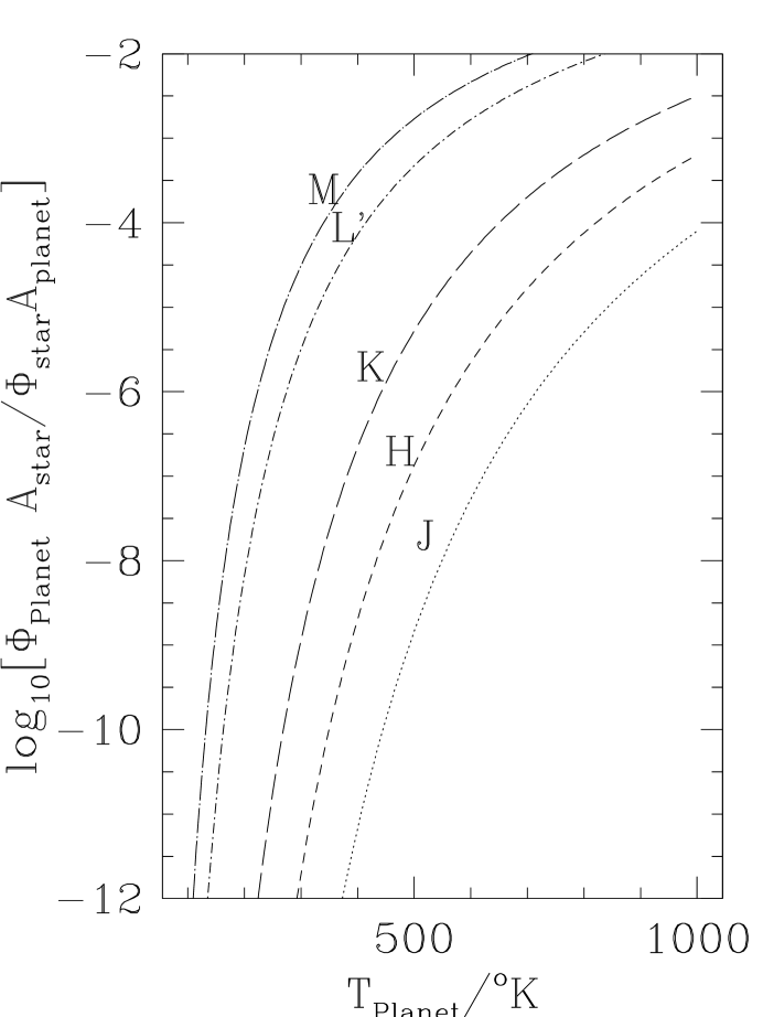
Figure 4: Relative brightness of a Jupiter-sized planet and a G-dwarf star ($T=5788\;{\rm K}$), as a function of the planet’s surface temperature for selected wave bands.

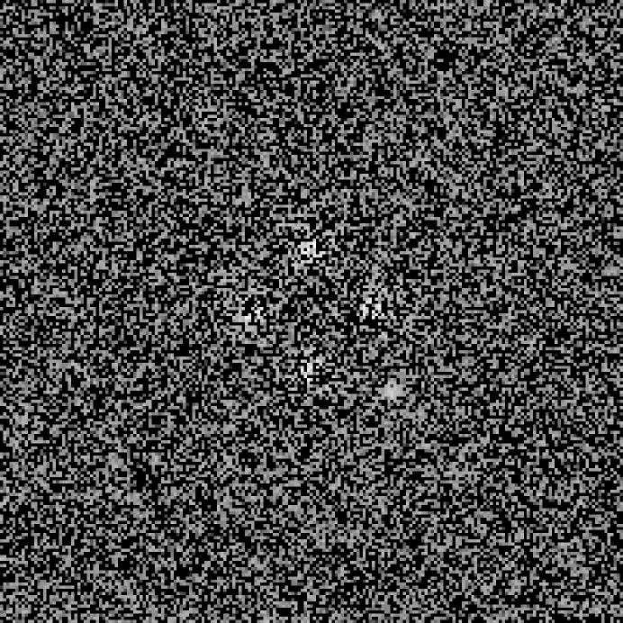
Figure 6: The log of the intensity for a diffraction pattern in the K-band with a planet $0.36\;{\rm as}$ from a star as seen in a $10$-m telescope. The star is $10\;{\rm pc}$ away, has an apparent bolometric magnitude of 5, and is located at the center of the satellite. The planet is radiating as a blackbody at $400\;{\rm K}$. We have assumed that the PSF can be characterized to 1% and have subtracted the PSF and a constant background. The planet can be seen along the lower right diagonal in the image.

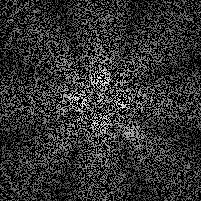
Figure 7: The log of the intensity for a diffraction pattern in the K-band with a planet $0.31\;{\rm as}$ from a star as seen in a $4$-m telescope in space. The star is $10\;{\rm pc}$ away, has an apparent bolometric magnitude of 5, and is located at the center of the satellite. The planet is radiating as a blackbody at $400\;{\rm K}$. We have assumed a fully diffractive PSF and no background. Here the satellite is only $100\;{\rm m}\times 100\;{\rm m}$. The planet can be seen along the lower right diagonal in the image.

In the near IR ($1$–$10\;{\rm\mu m}$) the luminosity is dominantly intrinsic emissions. In figure (4), this is shown as a function of planet surface-temperature, for a central star temperature of $5778\;{\rm K}$. Although the planet-star contrast is smaller in the near IR, the background is also much higher for ground-based telescopes. For K-band, the Mauna Kea IR background is approximately 13.5 mag per square arcsecond. Although longer wavelength bands are better in terms of planet intensity vs. stellar intensity, they are severely limited from the ground by increased background. In figures 6-7, we demonstrate the capabilities of the IRIS satellite in the near IR.

In figure 6, we show a Jovian planet with a surface temperature of $400\;{\rm K}$, orbiting at $3.6\;{\rm AU}$ from a 5 mag star $10\;{\rm pc}$ from the Earth. The images is a $1000\;{\rm s}$ exposure by a ground-based 10-m telescope. The PSF has a diffraction-limited core and a $1\;{\rm as}$ (FWHM) Gaussian halo with an on-axis intensity $10^{-3}$ that of the diffractive core. The image of the planet is clearly visible along the lower right diagonal.

In figure 7, we show the same system in a $1000\;{\rm s}$ exposure by a space-based 4-m telescope with a purely diffractive PSF, but now with a much smaller $100\;{\rm m}\times 100\;{\rm m}$ satellite placed $56,000\;{\rm km}$ from the telescope. Here the planet is $3.1\;{\rm AU}$ from a 5 mag star $10\;{\rm pc}$ from the Earth. Again the planet is clearly visible along the lower right diagonal.

At shorter wavelengths, the planets are best seen in reflection. The typical visual albedos of gas giants are high, $\sigma\simeq 0.5\pm 0.05$. We take the ratio of flux from the planet to flux from the star to be

$${\Phi_{P}\over\Phi_{\star}}\simeq\sigma{\pi R_{P}^{2}\over 4\pi r_{p}^{2}}$$ (18)

where $R_{P}$ is the radius of the planet, and $r_{p}$ is its orbital radius. For Jupiter orbiting at $1\;{\rm AU}$, this is $2.6\times 10^{-8}$. In figure (5) we plot $\Phi_{P}/\Phi_{\star}$ versus $R_{P}$ for orbital separations ranging from $0.2\;{\rm AU}$ to $10\;{\rm AU}$. These are easily related to the angular separation from the primary star by

$${\theta\over\;{\rm as}}={R_{P}/{\;{\rm AU}}\over r_{p}/\;{\rm pc}}$$ (19)

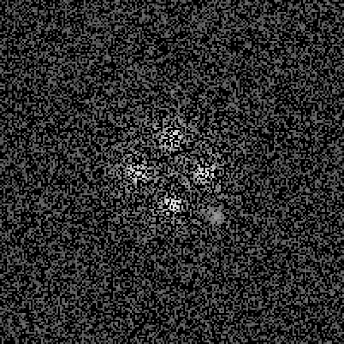
Figure 8: The log of the intensity for a diffraction pattern in the J-band with a planet $0.36\;{\rm as}$ from a star as seen in a $4$-m telescope. The star has an apparent bolometric magnitude of 5 and is located at the center of the satellite. The planet is reflecting light from the star with a relative intensity of $3\times 10^{-8}$. We have assumed that the PSF can be characterized to 1% and have subtracted the PSF and a constant background. The planet can be seen along the lower right diagonal in the image.

In figure 8, we show a J-band image of a Jovian planet in reflected light. The brightness of the planet is $3\times 10^{-8}$ of the central star, and it is $0.36\;{\rm as}$ from the star. The image is a $1000\;{\rm s}$ exposure on a 4-m ground-based telescope, using a PSF with a diffraction-limited core and a Gaussian halo with FWHM of $1\;{\rm as}$ and an on-axis brightness $10^{-3}$ that of the core. The J-band background is taken to be 15.2 mag per square arcsecond. Again the planet is clearly visible along the lower right diagonal.

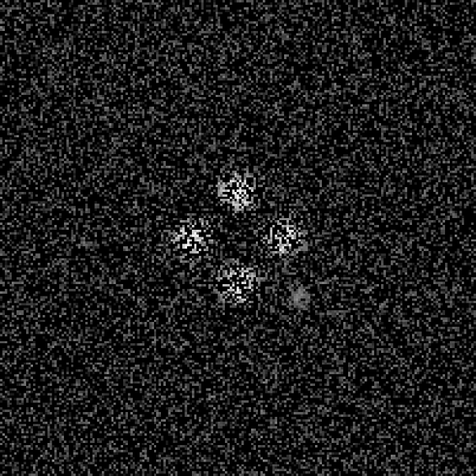
Figure 9: The log of the intensity for a diffraction pattern in the B-band with a planet $0.36\;{\rm as}$ from a star as seen in a $4$-m telescope. The star has an apparent bolometric magnitude of 5 and is located at the center of the satellite. The planet is reflecting light from the star with a relative intensity of $5\times 10^{-8}$. We have assumed that the PSF can be characterized to 1% and have subtracted the PSF and a constant background. We have also assumed seeing of $0.1\;{\rm as}$ (FWHM). The planet can be seen along the lower right diagonal in the image.

In figure 9, we show a B-band image of a Jovian planet in reflected light, taken with a $1000\;{\rm s}$ exposure on a ground-based 4-m telescope. The brightness of the planet is $5\times 10^{-8}$ of the central star, and it is $0.36\;{\rm as}$ from the star. The relevant backgrounds in the B-band is $22\;{\rm mag}\;{\rm as}^{-2}\;{\rm\AA}^{-1}$. The PSF has a Gaussian core with a FWHM of $0.1\;{\rm as}$, plus a Gaussian halo with FWHM of $1\;{\rm as}$ and an on-axis brightness $10^{-3}$ that of the core. This core represents a factor of 2.5 improvement over the seeing at the best sites. Using a Gaussian core of $0.25\;{\rm as}$, this planet is not visible to the eye. Image quality would also improve somewhat if we used a 10-m telescope (we have not done so because of the much increased computer time necessary to produce the image), but not enough to fully compensate for the seeing. In fact, it would be better to deploy an AO system which achieves a $0.1\;{\rm as}$ core on a 2 or 4-m telescope, than a less effective AO system on a larger instrument.

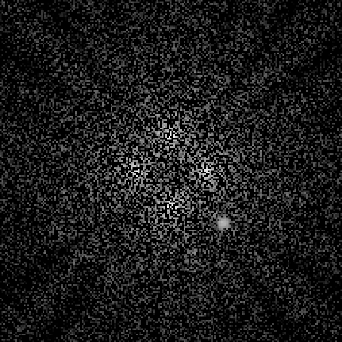
Figure 10: The log of the intensity for a diffraction pattern in the B-band with a planet $0.31\;{\rm as}$ from a star as seen in a $2$-m telescope in space. The star has an apparent bolometric magnitude of 5 and is located at the center of the satellite. The planet is reflecting light from the star with a relative intensity of $3\times 10^{-8}$. We have assumed a fully diffractive PSF and the same background as from the ground. Here the satellite is only $100\;{\rm m}\times 100\;{\rm m}$. The planet can be seen along the lower right diagonal in the image.

In figure 10, we show a B-band image of a Jovian planet in reflected light, taken with a $1000\;{\rm s}$ exposure on a space-based 2-m telescope. The brightness of the planet is $5\times 10^{-8}$ of the central star, and it is $0.31\;{\rm as}$ from the star. Once again, the satellite is only $100\;{\rm m}\times 100\;{\rm m}$ and only $56,000\;{\rm km}$ from the telescope. A diffractive PSF, and a background of $22\;{\rm mag}\;{\rm as}^{-2}\;{\rm\AA}^{-1}$ are used.

Finally, in figure 11 we plot the intensity ratios as viewed by ground-based telescopes of a star occulted by the satellite and an unocculted star in the B, J, and K-bands for a diagonal slice through the field of view averaged over $0.03\times 0.03\;{\rm as}^{2}$ pixels. (The diagonal slice being neither the most optimistic nor the most pessimistic.) This is arguably the true figure of merit for IRIS, as it represents the extent to which IRIS improves the contrast for the appropriate observing instrument. In the K-band the observing instrument is a 10-m telescope; in the J and B-bands it is a 4-m telescope. In the J and K-bands we used a PSF with a diffraction limited core and a Gaussian halo with a FWHM of $1\;{\rm as}$ and an on-axis intensity $10^{-3}$ that of the core. In the B-band the core is a Gaussian with a FWHM of $0.1\;{\rm as}$. The figure demonstrates that IRIS provides an improvement of $(1\hbox{--}4)\times 10^{-3}$ in the intensity in the wings for the J and K-bands and $(4\hbox{--}8)\times 10^{-4}$ in the B-band.

8 Image Resolution

For sources of comparable brightness (such as individual images in a gravitational microlensing event), one would like to be sensitive to much smaller angular separations, $\phi\lesssim 1\;{\rm mas}$. The satellite cannot be reliably positioned so as to obscure only one source while transiting the other. Typically one source, then both sources will be occulted and then they reappear in the same order. The capabilities of IRIS to perform ultra-high resolution imaging therefore rests on the ability to very accurately measure the light curve of a compound source during an occultation event. The relevant integration time for establishing the compound nature of the source is the time it takes for the satellite to traverse the separation between the two sources on the sky.

8.1 Binary Sources

Consider two point sources $A$ and $B$ separated by a small angle $\phi$, with photon fluxes (${\rm photons}\;{\rm m}^{-2}\;{\rm s}^{-1}$) $\Phi_{A}$ and $\Phi_{B}$ respectively in some appropriate waveband. The rate at which photons from each source are collected by an instrument mounted on a telescope is $\Phi_{i}A_{\rm eff}$, where $A_{\rm eff}$ is the telescope’s collecting area times the detection efficiency. If $\mu_{\rm app}$ is the apparent angular velocity of the satellite relative to the background stars, then the expected number of photons to arrive while the brighter of the two sources is eclipsed must be large enough to distinguish the dimmer source from either $0$ or $(\Phi_{A}+\Phi_{B})$ at some satisfactory confidence level. The number of photons we can collect while IRIS occults one source and not the other is

$$N_{\gamma}={\Phi_{\rm min}A_{\rm eff}\phi\over\mu_{\rm app}}$$ (20)

where $\Phi_{\rm min}=\min(\Phi_{A},\Phi_{B})$. This must be greater than some minimum value $N_{\rm min}$. The value of $N_{\rm min}$ depends on the accuracy to which one wants to measure $\phi$, $\Phi_{A}$ and $\Phi_{B}$, and on the background.

We have seen that typical occultations at apogee last $250-2300\;{\rm s}$ from a well-placed site (e.g. Mauna Kea) for $x_{\parallel}=x_{\perp}=300\;{\rm m}$. Since, for these values of $x_{\parallel}$, IRIS subtends $0.36\;{\rm as}$, its average angular velocity across the field of view is $0.16\hbox{--}1.5\;{\rm mas}\;{\rm s}^{-1}$. Since the telescope is being used essentially as a large light bucket in this mode, readout times $<1\sec$ for a CCD with $100\times 100$ pixels is quite reasonable.

Values of $\Phi_{i}$ and $\phi$ vary depending on the target. For gravitational microlensing the objects are stars in the Milky Way or in the LMC. An LMC target star (Alcock et al. 1996) with apparent bolometric magnitude $m_{b}=18$, and effective temperature $T_{\rm eff}\simeq 5\times 10^{3}\;{\rm K}$ has $\Phi\simeq 8.5\times 10^{3}\;{\rm m}^{-2}\;{\rm s}^{-1}$. Since the dim image is typically not much dimmer than the unlensed star, we will take this as $\Phi_{\rm min}$. Typical angular separations of microlensed images are $\phi\simeq 1\;{\rm mas}$. With $A_{\rm eff}\simeq 50\;{\rm m}^{2}$, equation (20) gives a substantial

$$N_{\gamma}\simeq(3\hbox{--}30)\times 10^{5}\phi\;{\rm mas}^{-1}.$$ (21)

This implies that $0.05\hbox{--}0.2\%$ changes in the flux should be readily detectable.

Equation (6) gives the diffraction angle, $\theta_{\rm diff}$, as a function of wavelength and of satellite size and distance. For B-band observations ($\lambda\simeq 4\times 10^{-7}\;{\rm m}$), and $r_{a}\simeq 1.7\times 10^{8}$, if the two sources are closer together than about $10\;{\rm mas}$, then their diffraction patterns would overlap significantly. The problem of reconstructing a binary source from the lightcurve would then be complicated by diffraction-induced smoothing. In addition, the diffraction patterns must be averaged over the spectrum of the source convolved with the transmission function of the filter with which the objects are being observed. This will degrade the resolution. Finally, the diffraction patterns must be integrated over the beam pattern of the telescope, further degrading the resolution. Including the effects of both beam smearing and wavelength convolution, Han et al. (1996) have shown that for lunar occultation (which is also in the Fresnel limit) one can achieve resolution of approximately $3\;{\rm mas}$. At first sight, since IRIS would be a half-way between the Moon and Earth it would seem that a resolution of only $3\sqrt{2}\simeq 4\;{\rm mas}$ would be achievable for IRIS. However, the Moon traverses the sky at $0.54\;{\rm as}\;{\rm s}^{-1}$, a factor of $300$–$3500$ times faster than IRIS’s apparent velocity, implying a proportional reduction in the number of collected photons, and a consequent significant reduction in resolution. Occultations with the satellite can also be repeated for these smallest angular resolutions, thus enhancing the signal-to-noise.

As we have seen, once the size of the satellite has reached $x_{\rm crit}\simeq\sqrt{\lambda r_{a}}$ no further improvement in resolution can be obtained by increasing the size. However, by opening several slits in the satellite we might narrow the diffraction pattern and increase the resolution. Moreover, since we are able to determine the diffraction pattern a priori very precisely (much more precisely than is possible for the Moon), we can model the light curve quite accurately and perform a fit to a binary source. This should help us to improve the resolution well below $10\;{\rm mas}$.

Furthermore, although we must still convolved the diffraction pattern as a function of wavelength with the spectrum of the source, and with the sensitivity of whatever detector and/or filters we may be using, we can avoid somewhat the degradation in image quality that this would imply by doing spectrometry. In this fashion the diffraction peaks at different wavelengths are not blended together, but rather can be used independently to reconstruct the surface brightness of the source. So long as the noise due to sky, contaminating sources, or other backgrounds are small, this wavelength spreading will not cause any decrease in signal. Observations made at shorter wavelengths could also help produce better resolution, though one must be careful not to lose photon flux by going to wavelengths well below the peak of the object’s spectrum.

The integration over the beam function of the telescope will continue to produce some degradation, if the peaks in the diffraction pattern of the source are closer together than the diameter of the telescope. Since $1\;{\rm m}$ subtends $1.2\;{\rm mas}$ at $1.7\times 10^{5}\;{\rm km}$, it may be preferable to make one’s observations with a series of independent smaller telescopes ($1\;{\rm m}$), rather than one large diameter instrument.

8.2 Compound Sources

IRIS will be able to produce maps of compound sources, such as planets or moons in our solar system, nearby stars and distant galaxies. The resolution of these images will be determined by the surface brightness of the source. Given the photon count rates derived above, we estimate that for most systems the resolution will be determined by requiring that the integrated flux over a resolved patch correspond to an 18–20 mag point source. We reserve further discussion of all of these effects to future papers now in preparation.

9 Conclusion

The IRIS satellite in a space-ground configuration, will offer distinct improvements for most currently envisaged ground based adaptive optics approaches to planet detection. The satellite blocks up to 99.97% of the light from a central star while leaving the balance in very well characterized, very concentrated images. Furthermore by doing the occulting well above the atmosphere, the problems of scattering in the telescope are minimized. At the same time, IRIS would benefit from all efforts to improve adaptive optics technology, particularly efforts to increase the fraction of the PSF in the diffraction-limited core. In the space-ground configuration we have shown that planets can be detected approximately $0.35\;{\rm as}$ from a nearby star in the B, J, and K-bands with only modest improvements in AO systems. Any improvements will be immediately usable by the ground-based telescopes making the observations and will improve the capabilities of IRIS. Furthermore IRIS can be used in conjunction with other ground based detection schemes such as coronographs and interferometers to improve upon them by suppressing 99.97% of the star’s light.

In space-space configuration, a smaller IRIS satellite, coupled with a 2–4-m class space telescope with basic instrumentation could greatly improve the prospects of seeing colder planets, particularly in reflected light. Such a configuration greatly improves the B-band images due to the poor seeing from the ground and the difficulty of building AO systems at these short wavelengths. We have shown that with a smaller satellite, closer to the telescope, we can also see planets approximately $0.3\;{\rm as}$ from a star in the B and K-bands. From space the diffraction limit of the telescope, particularly in the K-band, becomes the limiting factor. In the space-space configuration station keeping may allow longer integration times and the simpler orbital dynamics would reduce the size and number of orbit corrections.

In the field of planetary physics, IRIS would allow us to search for new planets around hundreds of nearby stars. In the field of gravitational microlensing, the measurement of the angular separations and orientations of the microlensed images as a function of time would greatly increase what can be learned about the physical properties of the lensing bodies. This is especially true if one could also obtain accurate measurements of the distance to the lens using some paralactic method, or by noticing the departure of the light curve from perfect time-reversal symmetry due to the Earth’s motion. In the field of Galactic structure, we could greatly improve our understanding of disk dynamics by obtaining parallaxes and proper motions of the nearby $1\;{\rm kpc}$, and possibly study the core of the galaxy, as well as globular clusters at higher resolution than has ever before been possible. The prospects of image separation with brightness contrasts of greater than $10^{8}$, of milli-arcsecond resolution of binary sources, and of milli-arcsecond resolved images of bright compound sources are all exciting. The possibilities are many.

We have shown that IRIS holds a great deal of promise but work remains to be done. More detailed PSF modeling, improved image identification algorithms, and better use of wavelength information will aid in both image separation and in high-resolution imaging observations. Using planetary motion between subsequent observations will aid in planet identification. The incorporation of more sophisticated models of planetary sources in both emission and reflection is needed to more fully understand the size and temperature of planets that can be observed. Improved numerical techniques are required to allow the simulation of observations by 10-m telescopes in the shorter wavelength bands. IRIS’s capabilities must be more completely characterized in the space-ground mode and in the space-space mode, for a variety of telescope sizes. This includes the improved exposure times for station keeping and for a variety of satellite-telescope separations in the space-space mode. Finally an investigation of a varying transmission coefficient over the surface of the satellite may lead to a truncated diffraction pattern from the satellite thus increasing the suppression of the light from the star and improving our ability to detect dim sources.

Figure 1: Integration time as a function of latitude for $r_{p}=6900\;{\rm km}$, $r_{a}=1.68\times 10^{5}\;{\rm km}$ and a period of 3 days.

Figure 2: Occultation of a binary source. Source A is occulted, source B is about to be occulted. In the geometric optics limit, rays from B strike the atmosphere at B’ while rays from A cannot strike the atmosphere between A’ and A”.

Figure 3: The flux from IRIS at apogee ($r_{a}=1.7\times 10^{5}\;{\rm km}$), as a function of the satellite’s temperature in the J, H, K, L and M-bands.

Figure 5: Ratio of the reflected flux of a planet to the flux from the primary star, for an albedo of $0.5$ for orbital separations of $0.2$–$10\;{\rm AU}$

[r]

Figure 11: Intensity ratio of an occulted and an unocculted star ($300\;{\rm m}\times 300\;{\rm m}$ satellite at $168,000\;{\rm km}$) as a function of angular separation from the star for a diagonal slice across the field-of-view in B,J and K-bands. All images have been convolved with a PSF consisting of a diffractive core in the J and K-bands and a gaussian core in the B-band with a FWHM of $0.1\;{\rm as}$). In both cases we include a gaussian halo (width of $1\;{\rm as}$ FWHM) with an on-axis intensity of $10^{-3}$ of the core on-axis intensity. The K-band image (solid line) is for a 10-m telescope; The B-band (long dashes) and J-band (short dashes) images are for a 4-m telescope. No background or noise is included.