Numerical stability of a family of Osipkov-Merritt models

Abstract

We have investigated the stability of a set of non-rotating anisotropic spherical models with a phase-space distribution function of the Osipkov-Merritt type. The velocity distribution in these models is isotropic near the center and becomes radially anisotropic at large radii. They are special members of the family studied by Dehnen and Tremaine et al. where the mass density has a power-law cusp $\rho\propto r^{-\gamma}$ at small radii and decays as $\rho\propto r^{-4}$ at large radii.

The radial-orbit instability of models with $\gamma$ = 0, 1/2, 1, 3/2, and 2, was studied using an N-body code written by one of us and based on the ‘self-consistent field’ method developed by Hernquist and Ostriker. These simulations have allowed us to delineate a boundary in the $(\gamma,r_{a})$-plane that separates the stable from the unstable models. This boundary is given by $2T_{r}/T_{t}=2.31\pm 0.27$, for the ratio of the total radial to tangential kinetic energy. We also found that the stability criterion $df/dQ\leq 0$, recently raised by Hjorth, gives lower values compared with our numerical results.

The stability to radial modes of some Osipkov-Merritt $\gamma$-models which fail to satisfy the Doremus-Feix’s criterion, $\partial f/\partial E<0$, has been studied using the same N-body code, but retaining only the $l=0$ terms in the potential expansion. We have found no signs of radial instabilities for these models.

1 Introduction

Spherical stellar systems in which the orbits are strongly eccentric, or radial, are unstable to forming a bar. This so-called radial-orbit instability (hereafter ROI), was first demonstrated for a sphere consisting entirely of radial orbits by Antonov (1973). It was actually observed by Hénon (1973) in a series of N-body simulations for the generalized polytropes, defined by a distribution function which is the product of power laws in energy and angular momentum. Subsequent N-body simulations (Merritt & Aguilar 1985; Barnes, Goodman, & Hut 1986; Dejonghe & Merritt 1988) and numerical linear stability analysis (Saha 1991; Weinberg 1991) have revealed that a small velocity anisotropy can be enough to make a system unstable; they also have showed that such a system evolves quickly into a triaxial bar.

The ROI can be explained by the transformation of loop orbits into box orbits when the spherical symmetry of the potential is broken (Merritt 1987). The mechanism is similar to the scenario described by Lynden-Bell (1979) for the formation of a bar in a disk. Initially, all the orbits are precessing ellipses (loops). A weak bar-like ($l=2$) perturbation generates a small torque that could trap those orbits with the lowest angular momenta; realign them around the bar, reinforcing the strength of the initial perturbation. This instability implies an upper limit to the degree of velocity anisotropy in spherical models. Dejonghe & Merritt (1988) studied the stability of the Plummer (1911) model with two different anisotropic distribution function (hereafter DF) and concluded that the ROI is the most robust and is likely to be the most important instability in elliptical galaxies.

For spherical stellar systems with isotropic DF, $f=f(E)$, it is known that $df/dE<0$ acts as a sufficient condition for the stability under radial and nonradial perturbations (Antonov 1962; Sygnet et al. 1984). However, the situation for anisotropic spherical models is poorly understood and only the stability to radial modes can be analytically tested using the sufficient condition $\partial f/\partial E<0$ (Dorémus & Feix 1973). A sufficient stability criterion based in the global anisotropy parameter $2T_{r}/T_{t}$, the ratio of kinetic energies corresponding to the radial and tangential direction, has been suggested by Polyachenko & Shukhman (1981; see Fridman & Polyachenko 1984). However, N-body simulations have showed that is not a reliable criterion because its value seems to be model dependent (Merritt & Aguilar 1985; Dejonghe & Merritt 1988). Moreover, Palmer & Papaloizou (1987) have analytically demonstrated that no stability criterion can be found using the anisotropy parameter $2T_{r}/T_{t}$, because there is always a spectrum of unstable (growing) modes if the DF becomes singular for a vanishing angular momentum; no matter how weak appears the DF divergence.

Recently, Hjorth (1994) has proposed a simple criterion for the stability of models with DF of the Osipkov-Merritt type (Osipkov 1979; Merritt 1985). These models are described by an anisotropic DF, $f(E,L^{2})=f(Q)$, with $Q\equiv E-L^{2}/2r_{a}^{2}$; where $E$ is the energy per unit mass and $L$ is the magnitude of the angular momentum per unit mass. Inside the anisotropy radius $r_{a}$ the velocity distribution is nearly isotropic, while outside $r_{a}$ the radial anisotropy increases. Thus, the parameter $r_{a}$ controls the global anisotropy degree in the velocity distribution; the smaller its value, the larger the anisotropy of the system.

In this paper we show the results of a numerical study of the stability properties for a set of Osipkov-Merritt models. These are special members of the family of spherical $\gamma$-models independently studied by Dehnen (1993, hereafter D93) and Tremaine et al. (1994, hereafter T94); with densities that behave as $\rho\propto r^{-\gamma}$ near the center and as $\rho\propto r^{-4}$ for large radii. The stability was investigated using an N-body code based on the ‘self-consistent field’ method developed by Hernquist & Ostriker (1992, hereafter HO92).

In § 2 we briefly describe the $\gamma$-models and the N-body code used to study their evolution. In § 3 we present our results for models with $\gamma$ = 0, 1/2, 1, 3/2, and 2. In particular, we are able to establish a stability boundary for the ROI in the $(\gamma,r_{a})$-plane. A discussion and summary of our results appear in § 4.

2 N-body Simulations

2.1 Models and Initial Conditions

In this section, we briefly summarize the properties of the one-parameter family of spherical models studied by D93 and T94 (more details can be found in the references just quoted). These $\gamma$-models have a mass density given by

$$\rho(r)=\frac{3-\gamma}{4\pi}\frac{aM}{r^{\gamma}(r+a)^{4-\gamma}},\;\;\;0\leq\gamma<3,$$ (1)

where $a$ is a typical scale length and $M$ is the total mass of the system (T94 describe the same density by the parameter $\eta=3-\gamma$ and call them “$\eta$-models”). The models of Jaffe (1983) and Hernquist (1990, hereafter H90) are recovered for $\gamma=2$ and $\gamma=1$, respectively.

The gravitational potential associated with the density (1) is obtained from the Poisson equation, and has the simple form

$$\Phi(r)=\frac{GM}{a}\times\left\{\begin{array}[]{ll}\displaystyle\ln\left(\frac{r}{r+a}\right),&\mbox{for $\gamma=2$,}\\ &\\ \displaystyle-\frac{1}{2-\gamma}\left[1-\left(\frac{r}{r+a}\right)^{2-\gamma}\right],&\mbox{for $\gamma\neq 2$},\end{array}\right.$$ (2)

where $G$ is the gravitational constant. In the following, we adopt a system of units in which $M$, $a$, and $G$ are unity.

Many dynamical properties of the $\gamma$-models with an isotropic DF, $f=f(E)$, were given by D93 and T94. The former also gave analytical expressions for anisotropic DFs of the Osipkov-Merritt type for some $\gamma$-models. More recently, Carollo, de Zeeuw, & van der Marel (1995) have been able to express the projected line-of-sight velocity profiles of models with $\gamma\leq 2$ in a single quadrature. Models with $\gamma>2$ are less suited to describe spherical galaxies because they display some unrealistic properties, such as infinite central potential and surface density profiles that differ significantly from the $R^{1/4}$ law (see D93).

We have limited our study to models with $\gamma$ = 0, 1/2, 1, 3/2, and 2, which represent a wide range for the density cusp at small radii. The $\gamma=0$ model is the only one of this family that has a (non-isothermal) core. The model that most closely resembles the $R^{1/4}$ law in surface density is the $\gamma=3/2$ model (D93). In spite of a previous study by Merritt & Aguilar (1985) of Jaffe ($\gamma=2$) model, we have included it here to obtain a more accurate estimation for its stability threshold. In fact, as we show below, we found a slightly larger value for the critical anisotropy radius than theirs.

For all these models, we have generated a set of initial conditions using the Osipkov-Merritt DF. Each model was truncated at a radius enclosing 99.9% of the total mass. All simulations employ $N=50,000$ equal mass particles. Table 1 shows the parameters associated with each of these models; where $r_{h}$ is the half-mass radius, $r_{0}$ is the lower value for the anisotropy radius such that the DF is strictly positive, and $T_{h}$ is the dynamical time evaluated at $r_{h}$.

2.2 N-body code

The stability of these models has been studied using an N-body code based on the ‘self-consistent field’ method developed by HO92 (see also Clutton-Brock 1973). In this approach, the density and the gravitational potential are expanded in a biorthogonal set of basis functions as

$$\begin{array}[]{lclcl}\rho({\bf r})&=&\displaystyle\sum_{nlm}A_{nlm}\rho_{nlm}({\bf r})&=&\displaystyle\sum_{nlm}A_{nlm}\tilde{\rho}_{nl}(r)Y_{lm}(\theta,\varphi),\\ &&&&\\ \Phi({\bf r})&=&\displaystyle\sum_{nlm}A_{nlm}\Phi_{nlm}({\bf r})&=&\displaystyle\sum_{nlm}A_{nlm}\tilde{\Phi}_{nl}(r)Y_{lm}(\theta,\varphi).\end{array}$$ (3)

HO92 obtained their basis functions $\{\rho_{nlm},\Phi_{nlm}\}$ using the model for spherical galaxies proposed by H90 as the zeroth-order term. Higher order terms are found by construction. For a set of $N$ pointlike particles the expansion coefficients $A_{nlm}$ are given in terms of the positions of the particles. Then, the accelerations are computed by a simple analytical differentiation of the potential expansion (see HO92 for a more detailed description).

One of us (AM) has written a code that implements this formalism. In this code the particle positions and velocities are updated using a second order integrator with a fixed timestep $\Delta t$, given by

$${\bf x}_{i+1} = {\bf x}_{i}+\Delta t\,{\bf v}_{i}+\frac{1}{2}\,\Delta t^{2}\,{\bf a}_{i},$$ (4)

$${\bf v}_{i+1} = {\bf v}_{i}+\frac{1}{2}\,\Delta t\,({\bf a}_{i}+{\bf a}_{i+1}),$$ (5)

where the subscript identifies the iteration. This integrator is equivalent to the standard time centered leapfrog, as can be verified by direct substitution (Allen & Tildesley 1992; Hut, Makino, & McMillan 1995). We have studied its numerical properties and found them closely similar to those of the standard leapfrog.

The HO92 basis set can be used to represent a number of potential-density pairs for spherical galaxies, including the $\gamma$-models. For example, the $\gamma=1$ model is just the zeroth order term and the $\gamma=0$ model can be reproduced exactly as a linear combination of two terms of this basis (HO92). However, for practical purposes, the potential (density) of other $\gamma$-models are approximated using truncated expansions of the kind defined in equation (3) limiting the number of radial functions to $n_{\rm max}$.

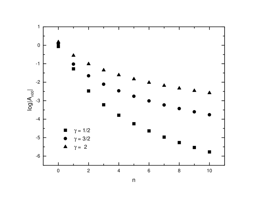
Figure 1: Expansion coefficients for some $\gamma$-models using the HO92 basis set.

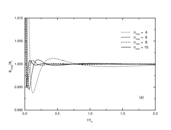
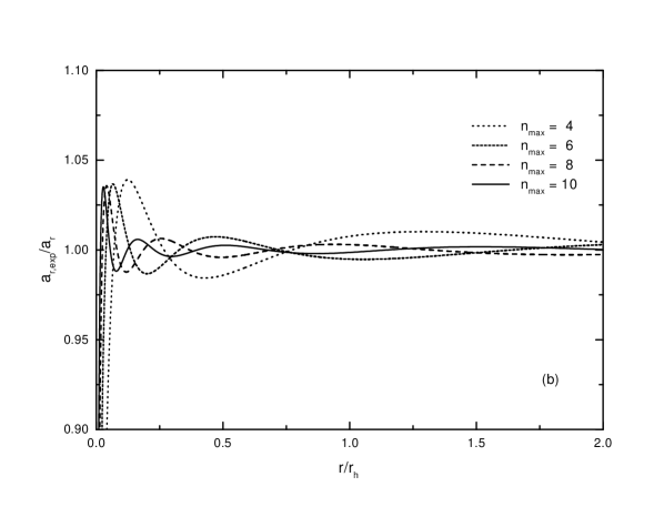
Figure 2: Relative error in the radial acceleration for the $\gamma$ = 1/2 (a) and $\gamma$ = 3/2 (b) model as a function of radius $r$. The figures compare the acceleration, as computed using the HO92 basis functions for different values of $n_{\rm max}$, to their exact values.

In our simulations, $n_{\rm max}$ has been chosen according to the studied model. Figure 1 shows the values of the expansion coefficients $A_{n00}$ (see eq. [2.35] of HO92) for some of the $\gamma$-models. The coefficients are directly related with $\gamma$; smaller values of $A_{n00}$ are obtained for lower $\gamma$. In all the cases, for large values of $n$ the coefficients $A_{n00}$ levels off. Then, adding more terms to the potential expansion does not decrease significantly the error, but the computational time increases considerably. However, in most cases, good accuracy in the evaluation of the potential can be achieved with $n_{\rm max}\sim 6$. This point is illustrated in Figure 2, where we compare the radial acceleration computed using the HO92 basis functions for the potential expansion (3), truncated at different values of $n_{\rm max}$, to its exact value for the $\gamma$ = 1/2 and $\gamma$ = 3/2 models. In both cases, at large radii, the acceleration obtained using the truncated potential expansion agrees with the one obtained using the full potential. However, at small radii, the error grows with $\gamma$. For $\gamma$ = 1/2, the radial acceleration can be computed to better than 0.5% accuracy at small radii, while for $\gamma$ = 3/2 the same quantity can be evaluated only up to 5% accuracy. The adopted values for $n_{\rm max}$ (see Table 1) were chosen such that the error in the acceleration, at small radii, was lower that 5%.

Since we are interested in the ROI, all our simulations only include series expansions up to $l_{\rm max}=2$. The total elapsed time was chosen as 50 half-mass dynamical times. The timestep for the different models appears in Table 1. They were taken such that the energy was conserved better than 0.5% during the total elapsed time. In some special cases, we checked that our results would not depend on the number of terms used in the potential expansion and the timestep (details are given below).

3 Results

To study the ROI in the models introduced in § 2.1, we have done a set of simulations with different values for the anisotropy radius $r_{a}$. For each run, we have used an iterative algorithm to estimate the axial ratios of the particle distribution. In this scheme, initial values for the modified inertia tensor

$$I_{ij}=\sum\frac{x_{i}x_{j}}{a^{2}},\hskip 56.9055pta^{2}=x^{2}+y^{2}/q_{1}^{2}+z^{2}/q_{2}^{2}$$ (6)

are calculated for all particles inside a spherical shell ($q_{1}=q_{2}=1$) with a given radius $r_{\rm m}$. New axis ratios $q_{1}$, $q_{2}$ and the orientation of the fitting ellipsoid are then estimated from the eigenvalues of $I_{ij}$ and used to obtain an improved approximation to the modified inertia tensor. This process is repeated until the axis ratios converge to a value within a pre-established tolerance, $\Delta q=0.001$.

We have tested the precision of this scheme computing the axis ratio of a set of random $N$ particle positions generated from the following triaxial generalization of the Hernquist model (e.g., Merritt & Fridman 1996)

$$\rho(m)=\frac{1}{2\pi bc}\frac{1}{m(1+m)^{3}},$$ (7)

with

$$m^{2}=x^{2}+\frac{y^{2}}{b^{2}}+\frac{z^{2}}{c^{2}},\hskip 56.9055pt0\leq c\leq b\leq 1.$$ (8)

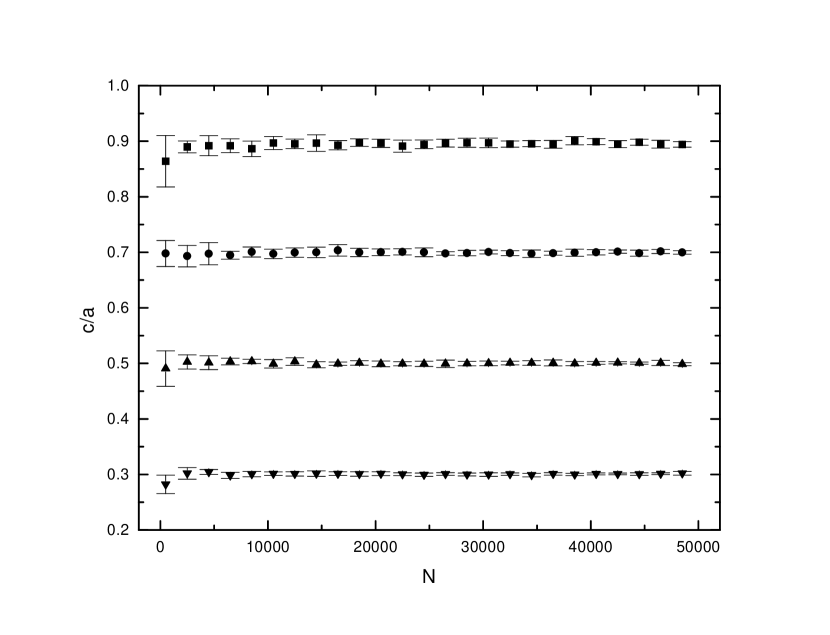
Figure 3: Computed minor axis ratio as a function of the number of particles $N$ for a set of 10 random generations of the “triaxial” Hernquist profile (eq. [7]) with $c=0.3$ (down triangles), $c=0.5$ (up triangles), $c=0.7$ (circles), and $c=0.9$ (squares). The error bar quoted here corresponds to the standard deviation of the measures.

Figure 3 shows the average computed minor axis ratio as a function of the number of particles $N$ within the radius $r_{\rm m}$. The error bar quoted correspond to the standard deviation for 10 different measures. We found that for $N\gtrsim 1000$, the computed axis ratio of the particle distribution came out with an error smaller than 1%. Convergence problems appear only when the number of particles inside the measuring radius $r_{\rm m}$ is small, or when $r_{\rm m}$ itself is small. To avoid this situation we have adopted as a measuring radius $r_{\rm m}$ the one that encloses the 70% of the total mass of the model. With these values for $r_{\rm m}$, we have obtained the axis ratio used as a test for stability.

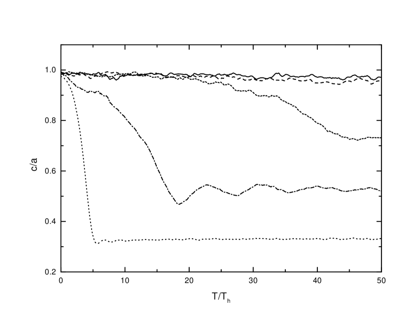
Figure 4: Evolution of the minor to major axis ratio for the Hernquist ($\gamma=1$) model for different values of the anisotropy radius $r_{a}$. The axis ratios were obtained by fitting an ellipsoid at radius $r_{\rm m}=5$, the radius which encloses $\sim$ 70% of the total mass. The time is normalized to the half-mass dynamical time $T_{h}$. Solid line: $r_{a}=1.1$; long-dashed line: $r_{a}=1.0$; short-dashed line: $r_{a}=0.9$; dotted-dashed line: $r_{a}=0.7$; and dotted line: $r_{a}=0.3$.

The evolution of the ratio between the minor to major axis for the Hernquist model with different values of the anisotropy radius $r_{a}$ appears on Figure 4. These values were obtained by fitting an ellipsoid at radius $r_{\rm m}=5$. The stability boundary appears to be close to $r_{a}=1.0$ and we assume that this model is stable. Models with $r_{a}\lesssim 0.8$ are strongly unstable and their final configuration is nearly prolate, with the final axis ratio determined by their initial anisotropy; the larger the value of the initial anisotropy, the smaller the final axis ratios. An example of the final state of a strongly unstable Hernquist model appears on Figure 5, where we have plotted the particle positions, projected along the minor semiaxis ($z$-axis), at the start and the end of a simulation for a model with anisotropy radius $r_{a}=0.3$. The particle positions are rotated in such a way that the semiaxis become aligned with the cartesian axis. At the end of the run, it is clearly visible a (triaxial) bar at the center of the system with $c/a=0.33$ and $b/a=0.40$.

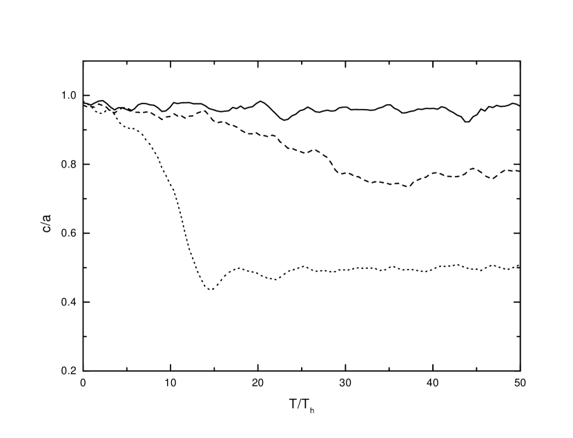
Figure 6: Evolution of the minor to major axis ratio for the Jaffe ($\gamma=2$) model. These values were obtained by fitting an ellipsoid at radius $r_{\rm m}=2.3$, the radius which encloses $\sim$ 70% of the total mass. The time is normalized to the half-mass dynamical time $T_{h}$. Solid line: $r_{a}=0.4$; dashed line: $r_{a}=0.3$; and dotted line: $r_{a}=0.2$.

Figure 6 shows the evolution of the minor to major axis ratio for the Jaffe ($\gamma=2$) model. The axis ratios were evaluated at radius $r_{\rm m}=2.3$. In their study of this model, Merritt & Aguilar (1985) found a critical value for $r_{a}$ between 0.2 and 0.3. However, the total elapsed time in their simulations was only 20 dynamical times. This ambiguity is settled in Figure 6, where we can see that the model with $r_{a}=0.3$ appears to be stable for elapsed times $t\lesssim 20T_{h}$, however, for $t\sim 30T_{h}$ the system show signs of an incipient bar. Accordingly, we set the stability threshold at $r_{a}\sim 0.4$.

The evolution of the axis ratio for other $\gamma$-models is very similar. Our results are summarized in Figure 7. Table 1 includes The critical anisotropy radius $r_{a}$ and the respective critical global anisotropy $2T_{r}/T_{t}$. The stability boundary between stable and unstable models is given roughly by the linear fit $r_{a}=1.54-0.54\gamma$. This boundary came out very close with the conservative estimate $r_{a}=1.6-0.67\gamma$, raised by Carollo, de Zeeuw, & van der Marel (1995) based on the supposition that the stability boundary for models with $\gamma<2$ is given by $2T_{r}/T_{t}=2.5$, the critical global anisotropy quoted by Merritt & Aguilar (1985) for the $\gamma=2$ model.

Our results give a critical global anisotropy parameter $2T_{r}/T_{\perp}=2.31\pm 0.27$ for the $\gamma$-models; however, the values of the anisotropy parameter are larger for lower values of $\gamma$. This limit is larger than the values 1.75 and 1.58 reported by Fridman & Polyachenko (1984) and Bertin et al. (1994), respectively. In our opinion, these results strengthen the belief that this criterion does not yield a reliable prediction for the stability threshold value because it is strongly model dependent.

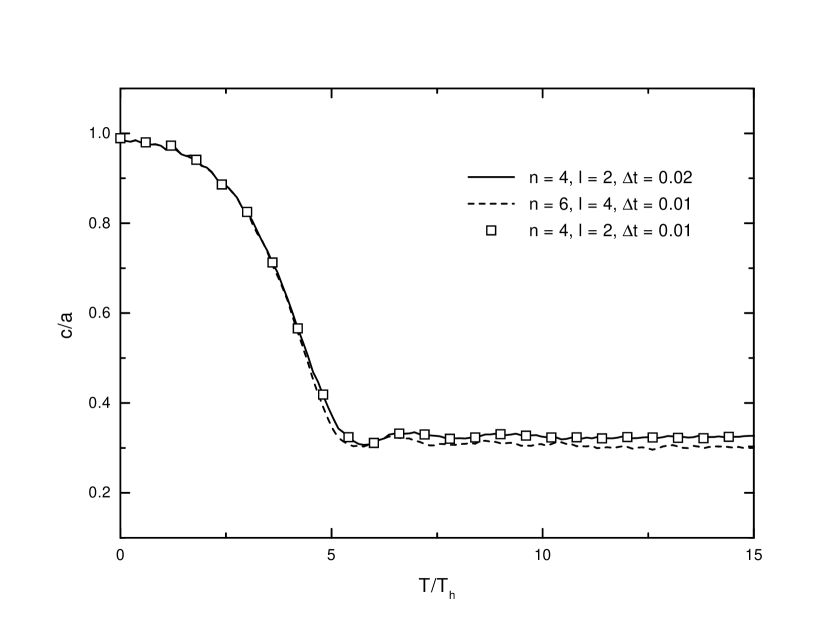
Figure 8: Evolution of the minor to major axis ratio for a Hernquist ($\gamma=1$) model with $r_{a}=0.3$. The same quantity is given for simulations with a shorter timestep $\Delta t=0.01$, and a potential expansion with $n_{\rm max}=6$ and $l_{\rm max}=4$.

We did additional runs to verify that our results were indeed independent of the timestep and the number of terms used in the potential expansion. Figure 8 shows the evolution of the minor to major axis ratio for the Hernquist ($\gamma=1$) model with anisotropy radius $r_{a}=0.3$. The run for this model was repeated using a shorter timestep, $\Delta t=0.01$, with essentially the same behavior for the axis ratio. A run with $n_{\rm max}=6$ and $l_{\rm max}=4$ converged to a slightly smaller final axis ratio. Similar results were obtained for other examples.

3.1 Radial stability

The sufficient condition $\partial f/\partial E<0$ (Dorémus & Feix 1973; Dejonghe & Merritt 1988) can be used to demonstrate the stability against radial perturbations of the Osipkov-Merritt $\gamma$-models. The lower value for the anisotropy radius which satisfies the Dorémus-Feix’s criterion, $r_{DF}$, is given in Table 1. We have studied the stability to radial perturbation modes of some of those models that fail to satisfy this criterion, using the same N-body code described in § 2.2, but retaining only the $l=0$ terms in the potential expansion. No signs of radial instability were observed in these runs.

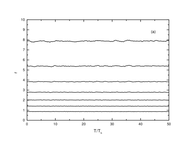
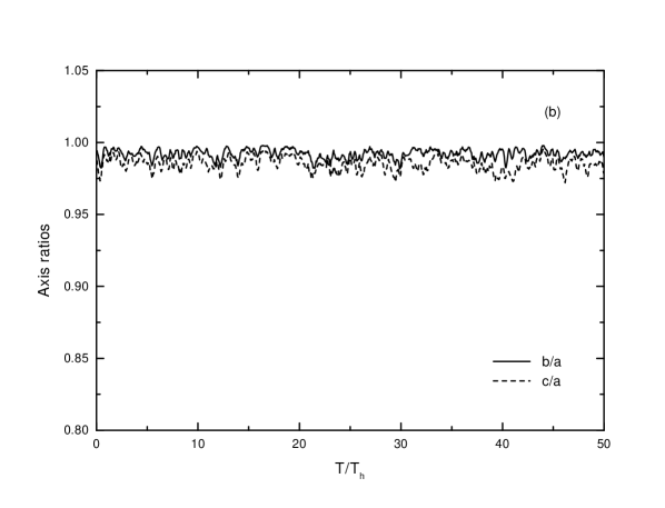
Figure 9: Evolution of the radial distribution of matter (a) and the axis ratios (b) for the $\gamma=0$ model with anisotropy radius $r_{a}=0.5$. These results were obtained retaining only the $l=0$ terms in the potential expansion.

An example of this result is displayed in Figure 9, which is a plot of the evolution of the radii containing 10%, 20%, …, 70% of the total mass and the minor to major axis ratio, for the $\gamma=0$ model with anisotropy radius $r_{a}=0.5$. In both cases, the mass distribution only shows the fluctuations associated with the finite number of particles. There are no discernible changes in the radial distribution of matter and the shape of the particle distribution. Similar results were observed in the other examples, which do not satisfy the Dorémus-Feix’s criterion. We conclude that all these models are stable to radial modes.

4 Discussion and summary

Recently, Hjorth (1994) has proposed an analytical criterion for the onset of instability for Osipkov-Merritt models. We have used our simulations to test this criterion. For the models discussed here, we have found that the numerical instability thresholds are higher than the predicted value given by Hjorth’s criterion, $df/dQ\leq 0$ (circles in Figure 7). Other independent numerical results point in the same direction. Dejonghe & Merritt (1988) using a multipolar expansion N-body code have found that the Osipkov-Merritt-Plummer model is unstable for an anisotropy radius $r_{a}\lesssim 1.1$, while Hjorth’s criterion predicts $r_{a}\lesssim 0.9$. For this model, we also have tried a different approach doing a series of simulations using an N-body code based on the Clutton-Brock (1973) basis set (see also HO92). Our results (Meza & Zamorano 1996) indicate that the stability boundary lies near $r_{a}=1.1$; the same value previously obtained by Dejonghe & Merritt (1988).

According to Hjorth (1994), this discrepancy may be originated by numerical errors in the representation of the central potential due to the small number of particles used in the simulations. He argues that these errors could induce artificial inflection points in the DF of the N-body realization. In this case, there should be a correlation between the number of particles and the stability threshold determined using these conditions: fewer particles should start an instability for higher values of the anisotropy radius $r_{a}$. To decide about this eventual behavior we have done some additional runs with $N=10^{5}$ and $2\times 10^{5}$ particles for anisotropy radius closer to the critical value quoted for the $\gamma$-models studied in the previous section. Figure 10 shows the results for the evolution of the minor to major axis ratio for the $\gamma$ = 3/2 model with anisotropy radius $r_{a}=0.8$. We observe that the curves show basically the same behavior and we conclude that the number of particles does not affect our estimation for the stability threshold. The same result repeats for the other $\gamma$-models. After these considerations, we feel that it would be interesting to review the hypothesis used in the Hjorth’s criterion.

Our results can be summarized as follows:

1. Using an N-body code based on the ‘self-consistent field’ method developed by HO92, we have tested the stability of a set of $\gamma$-models with DFs of the Osipkov-Merritt type. We found an approximated stability boundary for the ROI on the $(\gamma,r_{a})$-plane. This boundary is given by a global anisotropy parameter $2T_{r}/T_{t}=2.31$.

2. The criterion $df/dQ\leq 0$, recently suggested by Hjorth, gives a lower stability threshold for the $\gamma$-models.

3. We have studied the stability to radial modes of those $\gamma$-models which fail to satisfy the Dorémus-Feix’s stability criterion. No signs of instability were observed and we conclude that these models are stable to radial (shell forming) modes.

Table 1: Parameters of the models

$\gamma$	$r_{h}$	$r_{0}$	$r_{DF}$	$r_{a}$	$2T_{r}/T_{t}$	$T_{h}$	$\Delta t$	$n_{\rm max}$
0	3.85	0.44	0.75	1.5	2.63	16.8	0.05	4
1/2	3.13	0.32	0.63	1.3	2.47	12.3	0.02	6
1	2.41	0.20	0.52	1.0	2.39	8.3	0.02	4
3/2	1.70	0.10	0.42	0.8	2.09	4.9	0.01	6
2	1	0	0.34	0.4	1.98	2.2	0.01	14

Figure 5: Particle positions as viewed along the minor semiaxis at the beginning (a) and at the end (b) of a simulation for the Hernquist model with $r_{a}=0.3$. The particle positions are rotated such that the major (intermediate) semiaxis remains aligned with the $x$-axis ($y$-axis). This region contains approximately 70% of the total mass of the system.

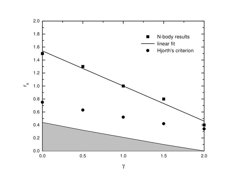
Figure 7: The $(\gamma,r_{a})$-plane for Osipkov-Merritt $\gamma$-models. Models in the shaded region have $f(Q)<0$ for some values of $Q$. The squares plotted are our numerical results and the stability threshold predicted by the Hjorth’s criterion $df/dQ\leq 0$ is marked with circles. The solid curve drawn is a linear fit obtained with our numerical results and roughly represents the lower boundary for models which are not affected by the radial-orbit instability.

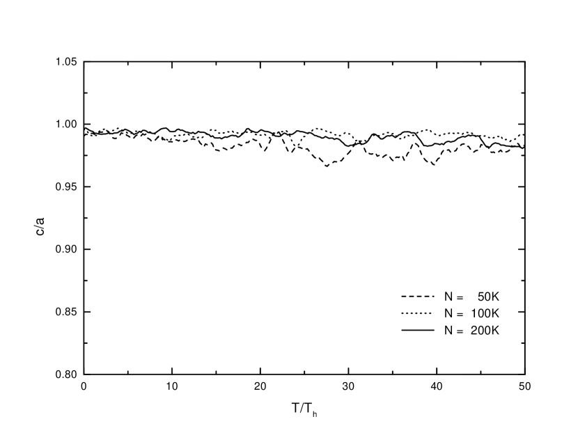
Figure 10: Evolution of the minor to major axis ratio for the $\gamma$ = 3/2 model using $N=5\times 10^{4},10^{5}$, and $2\times 10^{5}$ particles and anisotropy radius $r_{a}=0.8$. These values were obtained fitting an ellipsoid at radius $r_{\rm m}=3.7$.

References

- Allen & Tildesley (1992) Allen, M. P., & Tildesley, D. J. 1992, Computer Simulation of Liquids (Oxford: Oxford Univ. Press)
- Antonov (1962) Antonov, V. A. 1962, Vestnik Lenningradskogo Univ. 19, 96; english translation in IAU Symp. 127, Structure and Dynamics of Elliptical Galaxies, ed. T. de Zeeuw (Dordrecht: Reidel), 531
- Antonov (1973) Antonov, V. A. 1973, in The Dynamics of Galaxies and Star Clusters, ed. G. B. Omarov (Alma Ata: Nauka), 139; english translation in IAU Symp. 127, Structure and Dynamics of Elliptical Galaxies, ed. T. de Zeeuw (Dordrecht: Reidel), 549
- Barnes, Goodman, & Hut (1986) Barnes, J., Goodman, J., & Hut, P. 1986, ApJ, 300, 112
- Bertin et al. (1994) Bertin, G., Pegoraro, F., Rubini, F., & Vesperini, E. 1994, ApJ, 434, 94
- Carollo et al. (1995) Carollo, C. M., de Zeeuw, P. T., & van der Marel, R. P. 1995, MNRAS, 276, 1131
- Clutton-Brock (1973) Clutton-Brock, M. 1973, Ap&SS, 23, 55
- Dehnen (1993) Dehnen, W. 1993, MNRAS, 265, 250
- Dejonghe & Merritt (1988) Dejonghe, H., & Merritt, D. 1988, ApJ, 328, 93
- Dorémus & Feix (1973) Dorémus, J.P., & Feix, M. R. 1973, A&A, 29, 401
- Fridman & Polyachenko (1984) Fridman, A. M., & Polyachenko, V. L. 1984, Physics of Gravitating Systems, vols. 1 & 2 (New York: Springer)
- Hénon (1973) Hénon, M. 1973, A&A, 24, 229
- Hernquist (1990) Hernquist, L. 1990, ApJ, 356, 359
- Hernquist (1992) Hernquist, L., & Ostriker, J. P. 1992, ApJ, 386, 375
- Hjorth (1994) Hjorth, J. 1994, ApJ, 424, 106
- Hut, Makino, & McMillan (1995) Hut, P., Makino, J., & McMillan, S. 1995, ApJ, 443, 93
- Jaffe (1983) Jaffe, W. 1983, MNRAS, 202, 995
- Lynden-Bell (1979) Lynden-Bell, D. 1979, MNRAS, 187, 101
- Merritt (1985) Merritt, D. 1985, AJ, 90, 1027
- Merritt (1987) Merritt, D. 1987, in IAU Symp. 127, Structure and Dynamics of Elliptical Galaxies, ed. T. de Zeeuw (Dordrecht: Reidel), 315
- Merritt & Aguilar (1985) Merritt, D., & Aguilar, L. A. 1985, MNRAS, 217, 787
- Merritt & Fridman (1996) Merritt, D., & Fridman, T. 1996, ApJ, 460, 136
- Meza & Zamorano (1996) Meza, A., & Zamorano, N. 1996, in Chaos in Gravitational N-Body Systems, ed. J. C. Muzzio, S. Ferraz-Mello, & J. Henrard (Dordrecht: Kluwer), 259
- Osipkov (1979) Osipkov, L. P. 1979, Soviet Astron. Lett., 5, 42
- Palmer & Papaloizou (1987) Palmer, P. L., & Papaloizou, J. 1987, MNRAS, 224, 1043
- Plummer (1911) Plummer, H. C. 1911, MNRAS, 71, 460
- Polyachenko & Shukhman (1981) Polyachenko, V. L., & Shukhman, I. G. 1981, Soviet Astron., 25, 533
- Saha (1991) Saha, P. 1991, MNRAS, 248, 494
- Sygnet et al. (1984) Sygnet, J. F., Des Forets, G., Lachieze-Rey, M., & Pellat, R. 1984, ApJ, 276, 737
- Tremaine et al. (1994) Tremaine, S., Richstone, D. O., Yong-Ik, B., Dressler, A., Faber, S. M., Grillmair, C., Kormendy, J., & Lauer, T. R. 1994, AJ, 107, 634
- Weinberg (1991) Weinberg, M. D. 1991, ApJ, 368, 66