First Structure Formation:
II. Cosmic String + Hot Dark Matter Models.

Abstract

We examine the structure of baryonic wakes in the cosmological fluid which would form behind GUT-scale cosmic strings at early times (redshifts $z\lower 2.15277pt\hbox{$\;\buildrel>\over{\sim}\;$}100$) in an neutrino-dominated universe. We show, using simple analytical arguments as well as 1- and 2-dimensional hydrodynamical simulations, that these wakes will not be able to form interesting cosmological objects before the neutrino component collapses. The width of the baryonic wakes ($\lower 2.15277pt\hbox{$\;\buildrel<\over{\sim}\;$}10$ kpc comoving) is smaller than the scale of wiggles on the strings and are probably not enhanced by the wiggliness of the string network.

1 INTRODUCTION

One of the more interesting unknowns in cosmology is what happened during the “dark ages”, the period of time between the last scattering of the background radiation photons ($z\sim 10^{3}$), and the formation of the first objects we see, QSO’s ($z\sim 5$). As observational techniques improve, we are able to examine objects in the universe at earlier and earlier cosmological epochs (cf. Wampler et al.1996, Abraham et al.1996, and references therein). There is strong evidence that objects the size of very large present-day galaxies existed at $z\sim 4$. The plethora of early objects found suggest that the dark ages were not completely quiescent. However the dark ages could not have been too active a period since the spectrum of the Cosmic Microwave Background Radiation (CMBR), being extremely close to a blackbody spectrum, precludes the presence of a large amount of hot gas ($\gg 10^{3}$K) at these early times. This leaves the possibility of small sub-galactic objects, with small virial temperatures, being formed at very early times, $z\gg 5$.

Most inflationary models for the origin of inhomogeneities in the universe predict that the primordial density field will be Gaussian random noise with a nearly scale-invariant Harrison-Zel’dovich spectrum. The shape of the spectrum combined with the Gaussian statistics cause object formation to turn on fairly rapidly with very few precursor objects. In contrast, the non-Gaussian nature of inhomogeneities seeded by topological defects allow for a much greater number of precursor objects of a given mass to collapse long before the rms fluctuation on that mass scale has gone non-linear. Such precursor objects may play an important role in early star formation, producing metals to increase the efficiency of cooling in subsequent objects, and perhaps even triggering star-bursts via the shock waves produced by supernovae.

In the cosmic string model, these precursor objects can form around the wakes of cosmic strings which move through the primordial gas at all epochs (see Vilenkin and Shellard 1994 for a review of cosmic strings). It has been argued that star formation can take place in these wakes as early as $z\sim 10^{2}$ (Rees 1986, Hara 1987, Hara 1996a) and that one might very well form black holes as well (Hogan 1984, Hara et al.1996b). However the analysis which has led to these conclusions has not been sufficiently detailed to determine convincingly how, when, and whether these events occur. In this paper we examine some of these scenarios with hydrodynamical simulations. In particular we look at the most easily posed problem of a single cosmic string wake in a flat universe with hot dark matter (HDM). We emphasize at the outset that our conclusions do not apply to wakes in a universe with cold dark mater (CDM), or one with a mixture (MDM), or a universe without non-baryonic dark matter (so called BDM). We are also only considering the wakes before the neutrinos begin to collapse. Here we do not consider the collapse of the neutrinos themselves which will happen after the events we describe take place. There is ample literature on this subject (Stebbins et al.1987; Brandenberger, Kaiser, & Turok 1987; Bertschinger & Watts, 1988; Scherrer, Melott, & Bertschinger 1989; Perivolaropolous, Brandenberger, & Stebbins 1990; Colombi 1993; Zanchin, Lima, & Brandenberger 1996, Moessner and Brandenberger 1997, Sornborger 1997).

Of course it is difficult to demonstrate, using the hydrodynamical simulation techniques available today, the nature of star formation in a given cosmological scenario. However we are attempting the easier task of determining where stars do not form. In the cosmic string + HDM scenario, just after recombination, the gas is smoothly distributed since small scale perturbations are damped by photon diffusion (Silk damping) while the HDM is smoothly distributed because of it’s large velocity dispersion (i.e. damping due to free-streaming). Thus in this scenario we can hope to resolve all relevant scales in the problem, or at least before things collapse too much. Clearly stars cannot form unless the gas density of grows enormously over the ambient density. One might expect this to happen due to a cooling instability. However if the gas does not undergo an instability leading to very large over-densities then we can be fairly certain that stars will not form in that region. With the comprehensive non–equilibrium cooling and chemistry model of Abel et al.1997a, our study implements the details of molecular hydrogen formation and cooling accurately. Since our results indicate that instabilities generally do not occur, we do not need to worry about secondary effects which may be produced by star formation.

To study this problem we have used a version of ZEUS–2D, a Eulerian finite difference hydrodynamics code, that was modified to simulate nonequilibrium reactive flows in cosmological sheets by Anninos & Norman (1996). The code incorporates the methods developed by Anninos et al.(1997), and the comprehensive 9-species chemistry model of Abel et al.(1997). For this study we have further modified the code to account for the net force imparted on the baryons from Compton scattering with the CMBR), the so called Compton drag.

In the next section we give analytical arguments why a cooling instability is not found in the cosmic string + HDM model. Then we will describe our numerical methods and results in section 3. We refer the interested reader to our WWW page (http://lca.ncsa.uiuc.edu/$\sim$tom/Strings/) that also shows visualizations and movies of the 2–D simulations. Section 4 gives a brief summary of our results and discusses the implications for the cosmic string + HDM model.

2 ANALYTICAL ARGUMENTS

In this section we present some simple analytical arguments on the evolution of baryonic wakes. The velocity perturbations in the primordial gas induced by a moving string will cause the baryons to shock heat at the position of the string’s world sheet. For a “planar string” the velocity perturbations show reflection symmetry along the world sheet. Hence the evolution of the baryons will show the same symmetry unless hydrodynamic or thermo–gravitational instabilities affect the flow.

Throughout this paper we assume a hot dark matter component that fills the universe with $\Omega_{HDM}+\Omega_{B}=1$. The velocity dispersion of particles that were thermally produced in the early universe is given by (Kolb & Turner, 1990)

$$\langle v_{HDM}(z)\rangle\approx 23{\rm\ km/s}\left(\frac{m_{\nu}}{30{\rm\ eV}}\right)^{-\frac{4}{3}}\left(\frac{1+z}{10}\right),$$ (1)

where $m_{\nu}$ denotes the mass of the HDM particle. Since we are interested in early structure formation ($z\gg~{}5$), we can safely assume that the HDM component is distributed homogeneously and is not therefore dynamically important. Hence, $\Omega_{HDM}$ will only enter in the evaluation of the cosmological scale factor $a(t)$.

The trajectory of a gas particle after recombination and outside of the shocked region is the same as for a collisionless particle, which for a flat universe is given by (Stebbins et al.1987)

$$\triangle_{Q}(z)=\frac{1}{(p_{+}+p_{-})}\frac{v_{\rm kick}}{H_{0}\sqrt{\Omega_{0}}}\left[\frac{(1+z_{\rm kick})^{p_{+}-1/2}}{(1+z)^{p_{+}}}-\frac{(1+z)^{p_{-}}}{(1+z_{\rm kick})^{p_{-}+1/2}}\right],$$ (2)

where

$$p_{+}=\frac{1}{4}\left(\sqrt{1+24\Omega_{B}/\Omega_{0}}-1\right),\ \ \ p_{-}=\frac{1}{4}\left(\sqrt{1+24\Omega_{B}/\Omega_{0}}+1\right)$$ (3)

where $\Omega_{B}$, $v_{\rm kick}$, and $z_{\rm kick}$ denote the fraction of closure density in baryons, the initial kick velocity, and the kick redshift respectively. Since this result was derived using the Zel’dovich approximation we know it is exact in one dimension. Taking the time derivative, we find for the evolution of the peculiar velocity of the gas particles with respect to the cosmological frame, $u=(1+z)^{-1}d{\triangle_{Q}}/dt$. In Figure 1 we show the evolution of the velocity perturbation induced by a string at redshift 900 as a function of both redshift and $\Omega_{B}$ for the case of a flat background universe.

Figure 1: The peculiar velocity evolution for a string wake seeded at $z_{\rm kick}=900$ and $v_{\rm kick}=10{\rm\ km/s}$. The x–axis depicts the logarithm of redshift plus one, the y–axis the fraction of closure density in baryons, and the z–axis shows the logarithm of the peculiar velocity outside the shocked region. Note that for $\Omega_{B}=0$ the velocity simply decays $\propto(1+z)$ due to the cosmological expansion. Note also that changing the initial velocity kick only shifts this surface along the z-axis but does not change its shape.

We see that for all cases with $\Omega_{B}\lower 2.15277pt\hbox{$\;\buildrel<\over{\sim}\;$}0.5$, the infall velocity will be smaller at the present time than the initial kick velocity, illustrating that the wake was not able to acquire high enough surface densities to overcome the “drag” from the Hubble expansion.

From the Rankine–Hugoniot relations (Rankine 1870, Hugoniot 1889) we know that a strong adiabatic shock in an ideal gas will travel outwards with a fraction $\frac{1}{2}(\gamma-1)$ ($=1/3$ for the mono–atomic ideal gas with adiabatic index $\gamma=5/3$) of the infall velocity. The maximum velocity difference at the shock is given by the peculiar velocity $u$ with respect to the cosmological frame, yielding a maximum post-shock temperature of $kT=\mu u^{2}/3$. The immediate post–shock density equals $(\gamma+1)/(\gamma-1)$ ($=4$ for $\gamma=5/3$) times the pre–shock density, $\rho_{w}=\rho_{B}(\gamma+1)/(\gamma-1)=\rho_{0}(1+z)^{3}(\gamma+1)/(\gamma-1)$, where $\rho_{0}$ denotes the present mean density of baryons in the universe.

Abel (1995) and Tegmark et al.(1997) showed how one can, for a Lagrangian fluid element, integrate the kinetic rate equations of molecular hydrogen formation for applications where the collisional ionization of hydrogen atoms is unimportant, i.e. low velocity shocks with post–shock temperatures $\lower 2.15277pt\hbox{$\;\buildrel<\over{\sim}\;$}6000{\rm\ K}$. For redshifts $\lower 2.15277pt\hbox{$\;\buildrel<\over{\sim}\;$}100$ they find the H₂ fraction after one initial recombination time to be given by

$$f_{H_{2}}=1\times 10^{-3}\left(\frac{T_{0}}{2000{\rm\ K}}\right)^{1.53}\ln(x_{0}n_{H}k_{\rm rec}t+1),$$ (4)

where $T_{0}$ is the immediate post–shock temperature, $x_{0}$ the initial free electron fraction, $k_{\rm rec}$ the hydrogen recombination rate coefficient, and $n_{H}$ the number density of neutral hydrogen atoms. This formula describes remarkably well the numerical results of Abel et al.1997b. For redshifts greater than 100, this solution can be used as an estimate for the absolute maximum amount of H₂ that actually forms. We see that it takes at least one initial recombination time $(t_{\rm rec}=(k_{\rm rec}x_{0}n_{H})^{-1})$ to form a significant abundance of H₂ . Using $x_{0}=1.2\times 10^{-5}\sqrt{\Omega_{0}}/(h\Omega_{B})$ (Peebles 1993), $k_{\rm rec}=1.8\times 10^{-10}T^{-0.65}{\rm\ cm}^{3}{\rm\ s}^{-1}$, and the post–shock conditions derived above, we find that the minimum time to form hydrogen molecules is given by

$$t_{\rm min}=3.1\times 10^{15}{\rm\ s}\left(\frac{v_{\rm kick}}{10{\rm\ km/s}}\right)^{1.3}>\left(\frac{1+z}{100}\right)^{-3}.$$ (5)

Hence we see that, contrary to the case of ionizing shocks, there is a significant time lag between when the shock passes by and when enough H₂ can be formed to enable the gas to cool appreciably. At redshifts greater than 100, this time delay is longer due the photo-dissociation of the intermediaries H^- and H${}_{2}^{+}$ by the CMBR. This is essentially the reason why the instability of radiative shocks, as discussed by Chevalier and Immamura (1982), is not found for primordial gas when the shock does not ionize the gas. However, this instability can be observed for models with $\Omega_{B}>0.5$ since these models will be able to produce shocks with velocities faster than the initial kick velocity (see Figure 1) and reach the part of the cooling curve that allows the instability.

3 NUMERICAL SIMULATIONS

3.1 METHODS AND INITIALIZATION PARAMETERS

A numerical code with high spatial and mass resolution is required to model the hydrodynamics of a cosmic string wake and the micro–physics of chemical reactions and radiative cooling. We can achieve high dynamical ranges with the two–dimensional hydrodynamics code of Anninos and Norman (1996) which includes the 9 species chemistry and cooling model of Abel et al.(1997) and Anninos et al.(1997). However, we have replaced the ground state H${}_{2}^{+}$ photo-dissociation rate of Abel et al.(1997) with the LTE rate using the equilibrium constant given by Sauval & Tatum (1984) to account for the close coupling between the CMBR and the H${}_{2}^{+}$ molecule at high redshifts. We also account for the fact that the baryonic fluid motion at high redshift is slowed by the scattering of CMBR photons off the residual free electrons, the so called Compton Drag. This additional force can be expressed by a “drag time”, $t_{\rm d}=v/\dot{v}$, where $v$ denotes the peculiar velocity of the free electrons. For a gas with fractional ionization $x_{\rm e}=n_{\rm e}/n_{\rm t}$ and density $\rho_{\rm b}=n_{\rm t}\mu m_{\rm p}$, where $n_{\rm e}$ is the free electron number density, $n_{\rm t}$ is the total particle number density and $\mu$ is the mean molecular weight in units of proton mass $m_{\rm p}$, one may write this “drag time” as

$$t_{\rm d}={3\over 4}\,{1\over x_{\rm e}}\,{\mu\,m_{\rm p}\over\sigma_{\rm T}\,c\,\rho_{\gamma}}=2.4\times 10^{5}\,{\mu\over x_{\rm e}}\,\left({1000\,{\rm K}\over T_{\gamma}}\right)^{4}{\rm\ years}.$$ (6)

where $c$ is the speed of light, $\sigma_{\rm T}$ is the Thomson cross–section, and $T_{\gamma}$ is the CMBR temperature in Kelvin. Equation (6) is only valid in the optically thin limit, since in an optically thick medium the photons and baryons act as one fluid on scales much greater than the photon mean free path. In the code, we simply modify the updated velocity according to the first order discretization $\Delta{\bf v}=-\bf{v}\Delta t/t_{{\rm d}}$, where $\Delta t$ is the timestep defined by the minimum of the hydrodynamic Courant, gravitational free–fall, and cosmological expansion times. This will be sufficiently accurate as long as the “drag time” is much longer than the Courant time step. We start all our simulations at redshift $z=1100$ with an initial H₂ fraction of $10^{-10}$ and evolve the uniform background to the “kick redshift”. For the other eight species, we use the same initialization as in Anninos and Norman (1996). Furthermore, this procedure ensures that the temperature at the kick redshift $z_{\rm kick}$, is correctly derived from the balance of adiabatic expansion cooling and Compton heating.

An infinitely long and straight string traveling with a speed $v_{S}$ causes a velocity boost $v_{\rm kick}$ towards the sheet given by (Stebbins et al. 1987, but see §3.2)

$$|v_{\rm kick}|=4\pi\frac{G\mu}{c^{2}}v_{S}\left[1-\left(\frac{v_{S}}{c}\right)^{2}\right]^{-1/2},$$ (7)

where $G$ is the gravitational constant and $\mu$ is a mass per unit length of the string. Measurements of the CMBR anisotropy by the COBE satellite indicate that $G\mu/c^{2}\lower 2.15277pt\hbox{$\;\buildrel<\over{\sim}\;$}1.5\times 10^{-6}$ (Bennett, Stebbins, & Bouchet 1992, Coulson et al.1994, Allen et al.1996). Hence, for typical string velocities of $v_{s}\sim 0.8c$, one finds $v_{\rm kick}\sim 6{\rm\ km/s}$.

To simulate the idealized situation of a perfectly straight and infinite string, it is sufficient to perform one–dimensional simulations since the sheet traced out by the moving string is translation symmetric. Throughout this study we use a logarithmically refined grid spanning a physical distance of $0.4$ comoving  Mpc , with 200 zones arranged such that the zone size decreases from $18$ kpc at the outermost zones to $1.4$ pc at the central zone along the collapsing direction. The neighboring cells have a constant refinement ratio of $r=1.1$. We also set $\Omega{HDM}=0.94$, $\Omega_{B}=0.06$ and $h=0.5$ in all the simulations.

3.2 WIGGLINESS

It has been known for some time that cosmic string networks, while generally having a coherence length close to the cosmological horizon, also have structure on scales much smaller than the horizon (Vilenkin & Shellard 1995, and references therein). These wiggles do not extend to arbitrarily small scales, as they are damped by the emission of gravitational radiation. While the rms speed of cosmic string segments must be close to the speed of light, the “bulk velocity” of a long length of string, including the oscillating wiggles, can be significantly less. A particle located at a distance from the wiggly string that is greater than the extent of the wiggles would experience a net gravitational attraction greater than indicated by equation (7). However if one is interested in the gas dynamics in a small region around a segment of the string, a region smaller than the scale of the wiggles, the gravitational forces will be dominated by the force of that one segment and equation (7) will give a good indication of the velocity perturbation of the passing string.

Now we determine which regime we should be working in. For a non-wiggly string, $v_{\rm kick}\sim 10G\mu/c$ and the velocity of the strong shock wave produced would be ${1\over 3}$ of this, so the comoving width of the baryonic wakes is $\sim 5(1+z)\,G\mu t/c$. The comoving gravitational back-reaction scale for the strings, the scale of the smallest wiggles, is estimated to be $\sim 100(1+z)\,G\mu t/c$ (Vilenkin & Shellard 1995, and reference therein). While the two are the same order in $G\mu$, the numerical factors point to the wiggles being larger than the width of the baryonic wakes. If this is the case, then a purely planar wake might provide a sufficient description for the wakes. However, the effects of gravitational back-reaction are not completely understood and there may be other numerical factors which might cause these two scales to be more comparable. We allow for this in two ways in our simulations: first we consider kick velocities up to 20km/sec, which is greater than what would be expected for a straight piece of string, but might be more typical for the net effect of a wiggly string; secondly, in our 2–d simulations, we consider the flow onto a non-uniform string world-sheet, effectively modulating the value of $v_{\rm kick}$. More specifically we have modeled the initial flow as a potential flow, and one whose divergence $\nabla\cdot{\bf v}_{\rm kick}$ is non-zero on the planar string world-sheet, just as in the 1-d case. However in the 2-d case we allow the divergence to vary in one direction along the world sheet. More specifically, this divergence is drawn from a random distribution given by the positive square root of the sum of the square of two identically distributed real Gaussian random noise variables. From the perturbed surface density we compute the spatially varying velocity perturbations which show reflection symmetry about the string worldsheet. The variation along the wake was numerically captured with up to 128 grid points and the box size in this direction varied from 640 to 32 comoving kpc. We note, however, that introducing a spatially non-uniform second dimension does not lead to significantly higher overdensities than in the 1-d case.

3.3 RESULTS

We investigate wakes from infinitely long and fast moving straight strings with different initial data: $v_{\rm kick}=20$, 15, 10, $5{\rm\ km/s}$, and $z_{\rm kick}=900$, 500, 100, and 50. We discuss here only the results from one particular one–dimensional simulation, with $z_{\rm kick}=900$ and $v_{\rm kick}=20{\rm\ km/s}$. This optimistic case of an early string with a very high kick velocity is the most promising candidate to form the first structures in the cosmic string + HDM model and, indeed, led to the highest over densities ($\sim 200$) in all the simulated cases.

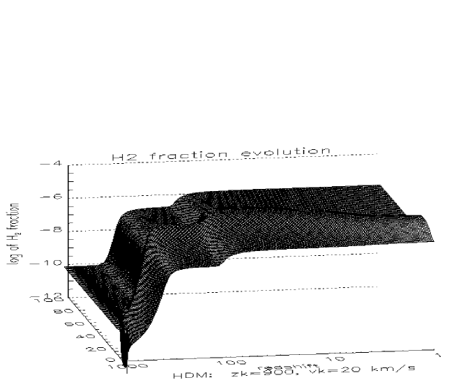
Figure 2: The evolution of the H₂ fraction for a string with $z_{\rm kick}=900$ and $v_{\rm kick}=20{\rm\ km/s}$. The x–axis depicts the redshift, the y–axis the cell number in the 1–d simulation and the z–axis shows the logarithm of the H₂ fraction.

Figure 2 shows, for one side of the perfectly symmetric wake, the evolution of the mass fraction of hydrogen molecules vs. cell number (distance from the string worldsheet), and also vs. redshift on the x–axis. At the kick redshift $z=900$, a shock forms that runs outwards. Two distinct steps are evident: the first at redshift $z\sim 500$, and the second at $z\sim 120$. The plateau before the first step is an artifact of our too high initialization of H₂ and is not physical. This, however, does not influence the subsequent evolution and results. The first step is due to the H${}_{2}^{+}$ chemistry, and occurs when the formation of H₂ molecules starts to dominate the destruction of H${}_{2}^{+}$ compared to its photo–dissociation by the CMBR. In the shocked region, it is evident that the $v_{\rm kick}=20{\rm\ km/s}$ shock is initially capable of destroying some hydrogen molecules. Shortly after $z_{\rm kick}=900$, however, the decaying infall velocity, the steadily rising H${}_{2}^{+}$ abundance, and the increasing H₂ formation rate lead to an overall enhanced H₂ fraction. The second step is due to the H^- path, which occurs slightly earlier in the denser, shocked regions than in the background. This is easily understood from the equilibrium abundance of H^- which is given by $n_{H^{-}}=n_{e}n_{H}k_{7}/(k_{23}+k_{8}n_{H})$, where $k_{7}$, $k_{8}$, and $k_{23}$ denote the reaction rates for the photo–attachment of H^- , the dissociative attachment reaction of H^- (H₂ formation), and the photo–detachment by the CMBR of H^- , respectively (the notation is taken from Abel et al.1996). That second step originates when $k_{23}\lower 2.15277pt\hbox{$\;\buildrel>\over{\sim}\;$}k_{8}n_{H}$, and $n_{H^{-}}$ is roughly proportional to $n_{H}n_{e}$ which is higher in the shocked gas than in the background, yielding to the enhanced H₂ formation rate. Another, and at first surprising, effect is that the central regions of the wake form fewer hydrogen molecules than regions further away. This is because the gas closer to the string world–sheet shocks at redshifts $z>110$, at which H^- is still destroyed efficiently by the CMBR and H₂ cannot form. The higher density in this shocked component leads to an increased hydrogen recombination which leaves fewer free electrons as catalysts for H₂ formation at lower redshifts. Consequently, this H₂ depression in the central layers are not observed for simulations with kick redshifts $\lower 2.15277pt\hbox{$\;\buildrel<\over{\sim}\;$}110$.

Compton Drag never becomes dynamically important even in the cases for which we chose extremely high kick velocities for which the shock was ionizing the gas. This is because the wakes do not become self–gravitating until very late redshifts. In other words, the post shock gas continues to expand with the Hubble flow and the gas shows no motion with respect to the rest frame of the background photons. Hence, there will be no net force on the baryons independent of their ionized fraction. Since the self-gravity of the gas plays little role in the evolution of the wake at early times, we should expect that inhomogeneities in the wake should have little effect since there is no significant gravitational instability to amplify any initial inhomogeneities.

Shapiro and Kang (1987) presented calculations of steady–state shocks of 20, 30, and 50 km/s occurring at redshifts 100 and 20 with and without external radiation fields. Interpreting their results as upper limits on the possible H₂ formation and cooling we find our simulations to agree with their findings at the low redshifts and high kick velocities where they are comparable.

4 CONCLUSION

We have studied the possibility of high redshift structure formation in the wakes of fast, long, and straight, as well as fast, long, and wiggly cosmic strings in a hot dark matter dominated universe. We find that insufficient amounts of H₂ molecules are formed, and the gas does not cool appreciably. Due to the fact that the baryonic cosmic string wakes do not become significantly self–gravitating to allow the infall velocities to exceed the initial kick velocity (see Figure 1.), we find the maximum overdensities reached in all the simulations we have carried out are $<10^{3}$, corresponding to hydrogen number densities less than $\sim 1\times 10^{-4}(\Omega_{B}h^{2}/0.025)(1+z)^{3}{\rm\ cm}^{-3}$. Thus no primordial stars can be formed in the studied wakes.

This leads us to conclude that, in the cosmic string + HDM model, one must wait for the neutrinos to collapse before anything like star formation can take place. In this work we have explicitly considered gauge (local) cosmic strings, but we expect these conclusions will apply to global cosmic strings as well. The baryonic structures considered above will be destroyed if and when they become enveloped in the collapse of the neutrinos, which will happen on much larger scales and involve much larger velocities. It has been suggested that neutrino collapse may happen as early as $z\sim 100$ (Zanchin, Lima, & Brandenberger 1996; Sornborger 1997) but other studies (Colombi 1993) find non-linear collapse only for $z\lower 2.15277pt\hbox{$\;\buildrel<\over{\sim}\;$}5$. Thus it is still an unsettled issue whether cosmic strings could have brought light to the dark ages, at least in the HDM scenario.

- [1]
- [2] Abel, T., 1995, thesis, Univ. Regensburg.
- [3]
- [4] Abel, T., Anninos, P., Norman, M., & Zhang, Y. 1997b, ApJ, accepted.
- [5]
- [6] Abel, T., Anninos, P., Zhang, Y., and Norman, M.L. 1997a, NewA accepted.
- [7]
- [8] Allen, B., Caldwell, R.R., Shellard, E.P.S., Stebbins, A., and Veeraraghavan, S. 1996 Phys. Rev. Lett., 77, 3061.
- [9]
- [10] Anninos, P., Zhang, Y., Abel, T., and Norman, M.L. 1997, NewA accepted.
- [11]
- [12] Abraham, R., Tanvir, N., Santiago, B., Ellis, R., Glazebrook, K., & Van den Bergh, S. 1996, MNRAS, 279, L47.
- [13]
- [14] Anninos, P. and Norman, M.L. 1996, ApJ, 460, 556.
- [15]
- [16] Bennett, D.P., Stebbins, A., and Bouchet, F., 1992, ApJ, 399, L5.
- [17]
- [18] Bertschinger, E. and Watts, 1988, ApJ, 316, 489.
- [19]
- [20] Brandenberger, R., Kaiser, N. and Turok, N., 1987 Phys. Rev. D, 36, 2242.
- [21]
- [22] Chevalier, R.A., and Imamura, J.N. 1982, ApJ, 261, 543.
- [23]
- [24] Colombi, S. 1993, Ph.D. Thesis, l’Universite de Paris 7.
- [25]
- [26] Coulson, D., Ferreira, P., Graham, P., and Turok, N., 1994, Nature, 386, 27.
- [27]
- [28] Hara, T., and Miyoshi, S., 1987, Prog. Theor. Phys., 78, 1081.
- [29]
- [30] Hara, T., Yamamoto, H., Mähönen, P., and Miyoshi, S. 1996a, ApJ, 461, 1.
- [31]
- [32] Hara, T., Yamamoto, H., Mähönen, P., and Miyoshi, S. 1996b, ApJ, 462, 601.
- [33]
- [34] Hogan, C., 1984, Phys. Lett. B., 143B, 87.
- [35]
- [36] Hugoniot, Par H. 1889, J. de l’Ecole Polytechnique, 57, 1.
- [37]
- [38] Kolb, E.W., and Turner, M. 1990, The Early Universe, Addison–Weseley Publishing Company, Redwood City, California.
- [39]
- [40] Moessner; R., and Brandenberger, R. 1997, astro-ph/970208.
- [41]
- [42] Peebles, P.J.E. 1993, Principles of Physical Cosmology, (Princeton University Press, NJ).
- [43]
- [44] Perivolaropoulos, L., Brandenberger, R., and Stebbins, A. 1990, Phys. Rev. D, 41, 1764.
- [45]
- [46] Rankine, W.J.M. 1870, Phil. Trans. Roy. Soc. London, 160, 277.
- [47]
- [48] Rees, M.J. 1986, MNRAS, 222, 27.
- [49]
- [50] Sauval, A.J, & Tatum, J.B. 1984, ApJS, 56, 193.
- [51]
- [52] Shapiro, P.R. and Kang, H. 1987, Rev. Mexicana Astron. Astrof., 14, 58.
- [53]
- [54] Scherrer, R., Melott, A., and Bertschinger, E. 1989, Phys. Rev. Lett., 62, 379.
- [55]
- [56] Sornborger, A. 1997, astro-ph/9702038.
- [57]
- [58] Stebbins, A., Veeraraghavan, S., Brandenberger, R., Silk, J., and Turok, N. 1987, ApJ. 322, 1.
- [59]
- [60] Tegmark, M., Silk, J., Rees, M.J., Blanchard, A., Abel, T., Palla, F. 1997, ApJ, 474, 1.
- [61]
- [62] Vilenkin A. and Shellard, E.P.S., 1994 Cosmic Strings and Other Topological Defects (Cambridge Monographs on Mathematical Physics).
- [63]
- [64] Wampler, E.J., Williger, G.M., Baldwin, J.A., Carswell, R.F., Hazard, C., and McMahon, R.G. 1996, A&A, 316, 33.
- [65]
- [66] Zanchin, V., Lima, J.A.S., and Brandenberger, R. 1996, Phys. Rev. D, 54, 6059.