SELECTED TOPICS IN NEUTRINO ASTROPHYSICS

This review covers a subset of the astrophysical phenomena where neutrinos play a significant role and where the underlying microphysics is nuclear physics. The current status of the solar neutrino problem, atmospheric neutrino experiments, the role of neutrinos in determining the dynamics of type-II supernovae, and recent developments in exploring neutrino propagation in stochastic media are reviewed.

1 Introduction

Neutrinos are perhaps the most interesting particles that we know to exist. (Of course there are many other interesting particles such as axions, supersymmetric partners, etc., that we wish to exist). It is gratifying to see that Federal Agencies in the U.S. and their counterparts around the world share the rational exuberance of neutrino physicists by funding a number of potentially very interesting experiments.

This review is intended for non-experts in neutrino physics and astrophysics. Topics covered here are chosen from those phenomena where the underlying microphysics is nuclear physics. The current status of the solar neutrino problem, atmospheric neutrino experiments, the role of neutrinos in determining the dynamics of type-II, core-collapse supernovae, and recent developments in exploring neutrino propagation in stochastic media are reviewed. One should emphasize that this is not intended to be a complete list. Other very interesting astrophysical and cosmological phenomena in which neutrinos play a role, such as primordial nucleosynthesis, the possibility of hot dark matter, and possible connection between neutrinos and pulsar proper motions are excluded from this review. Similarly, high-energy neutrino astrophysics, such as using neutrinos to probe active galactic nuclei, are omitted.

Neutrino physics and astrophysics are rapidly developing areas. It would be very difficult for any printed review to remain current for a sufficiently long time. To keep up to date on the current developments would require a dynamic medium such as the World Wide Web. Indeed, there are a number of sites devoted to neutrino physics. To keep up with the experimental developments some excellent sites to consult include “The Neutrino Oscillation Industry” page $\!{}^{{\bf?}}$ at Argonne National Laboratory and “The Ultimate Neutrino Page” $\!{}^{{\bf?}}$ at Helsinki. For theoretical results recommended sites include Bahcall’s homepage$\!{}^{{\bf?}}$ at the Princeton Institute for Advanced Study and the “Implications of Solar Neutrino Experiments” page $\!{}^{{\bf?}}$ at the University of Pennsylvania.

2 Neutrino Oscillations

In the minimal $SU(2)\times U(1)$ Standard Model neutrinos are taken to be massless (i.e., the neutrino field is left-handed). However, the Standard Model is an effective field theory $\!{}^{{\bf?}}$, applicable up to a certain energy scale beyond which new physics occurs. A massive neutrino would be one of the indications of such new physics and the value of the neutrino mass would be related to the scale of new physics $\!{}^{{\bf?}}$. For example, in the Grand Unified theories (GUTs) the right-handed neutrino sits in a singlet representation of the weak $SU(2)$ taken to be a subgroup of the fundamental representation of the grand-unifying gauge group. Since both helicity components are present in the theory, the spontaneous symmetry breaking mechanism yields a mass term for neutrinos in the same way it does for other leptons. Since both helicity components of the neutrino contribute to this mass term, it is known as the “Dirac mass”. For an electrically neutral particle such as the neutrino it is possible to introduce another mass term by combining the left-handed neutrino field with the right-handed antineutrino field, which both appear as weak isodoublets in the Standard Model. Such a mass term is known as the “Majorana mass”. A Majorana mass term leads to a breakdown in lepton number conservation. Neutrino masses can be introduced in GUTs via the See-Saw mechanism $\!{}^{{\bf?}}$. The See-Saw mechanism produces light neutrino masses of the order of $m_{\nu}\sim M^{2}_{D}/M_{M}$, where $M_{D}$ is a Dirac neutrino mass, and $M_{M}$ is a Majorana neutrino mass which is a weak isosinglet. Since the latter is associated with a new physics scale which is typically much larger than the electroweak scale associated with the former, this mechanism naturally produces very small neutrino masses.

In general the neutrino weak eigenstates that are observed in nuclear decays are not mass eigenstates. In these lectures we consider two-neutrino mixing for definiteness and assume that there is the usual unitary transformation between the flavor eigenstates (e.g., $\Psi_{e}$ and $\Psi_{\mu}$) and the mass eigenstates ($\Psi_{2}$ and $\Psi_{1}$):

$$\left[\begin{array}[]{cc}\Psi_{e}\\ \\ \Psi_{\mu}\end{array}\right]=\left[\begin{array}[]{cc}\cos{\theta_{v}}&\sin{\theta_{v}}\\ \\ -\sin{\theta_{v}}&\cos{\theta_{v}}\end{array}\right]\left[\begin{array}[]{cc}\Psi_{1}\\ \\ \Psi_{2}\end{array}\right]\,,$$ (1)

where $\theta_{v}$ is the vacuum mixing angle between the two flavors. A generalization to the case of three flavors is straightforward.

2.1 Vacuum Oscillations

Since the electron neutrino produced, for example, in a nuclear decay is a linear combination of the mass eigenstates and these mass eigenstates propagate with different phases, there is a probability that the other weak eigenstate will appear after some distance $L$. The evolution of the flavor eigenstates is governed by the equation

$$i\hbar\frac{\partial}{\partial t}\left[\begin{array}[]{cc}\Psi_{e}(t)\\ \\ \Psi_{\mu}(t)\end{array}\right]=\frac{1}{4E}\left[\begin{array}[]{cc}-\delta m^{2}\cos{2\theta_{v}}&\delta m^{2}\sin{2\theta_{v}}\\ \\ \delta m^{2}\sin{2\theta_{v}}&\delta m^{2}\cos{2\theta_{v}}\end{array}\right]\left[\begin{array}[]{cc}\Psi_{e}(t)\\ \\ \Psi_{\mu}(t)\end{array}\right]\,,$$ (2)

where $E$ is the neutrino energy, and $\delta m^{2}=m_{2}^{2}-m_{1}^{2}$ ($m_{2}>m_{1}$). In this equation a term proportional to the identity has been dropped since it does not contribute to the relative phase between the $\nu_{e}$ and $\nu_{\mu}$ components. The appearance probability of the other flavor is then given by

$$P=\sin^{2}2\theta_{v}\sin^{2}(1.27\delta m^{2}L/E),$$ (3)

In the above equation $\delta m^{2}$ is measured in eV² and $L/E$ in m/MeV. Neutrino oscillation experiments are somewhat arbitrarily divided into two classes: short-baseline and long-baseline. As Eq. (3) indicates, the longer is the baseline, $L$, the more sensitive the experiment is to smaller values of $\delta m^{2}$.

So far no group, with one possible exception, has reported a positive result in either the appearance nor in the disappearance experiments. The Liquid Scintillator Neutrino Detector (LSND) collaboration at Los Alamos National Laboratory reported a significant “oscillation-like” excess $\!{}^{{\bf?}}$. This detector sits 30 meters away from the beam dump at Los Alamos Meson Physics Facility (LAMPF). The experimental apparatus is designed to produce a beam of muon antineutrinos with as little contamination as possible from the electron antineutrinos. If these muon antineutrinos oscillate into electron antineutrinos, such formed electron antineutrinos would interact with protons in the detector, creating a positron and a neutron. This neutron, after some time, binds with a proton to form a deuteron, giving a photon with a characteristic energy of 2.2 MeV. The experiment observes these photons as well as the positron’s Cerenkov track. When they identify both signatures together, the LSND group first reported seeing nine events versus an expected background of two events coming from the electron antineutrinos from sources other than the muon antineutrino oscillation. This signal received a lot of attention and a fair amount of criticism. Indeed, a dissenting member of the LSND team has performed a data analysis of his own which finds no positive signal above the expected background $\!{}^{{\bf?}}$. The LSND result is unlikely to be a statistical fluctuation. However, the KARMEN collaboration, carrying out a similar (but not identical) experiment at Rutherford Laboratory in England, reported no evidence for neutrino oscillations in a parameter space which largely overlaps with that of LSND $\!{}^{{\bf?}}$. Later the LSND collaboration reported 22 events. $\!{}^{{\bf?}}$ The LSND collaboration is currently analyzing $\mu$ decay in flight, which will have different systematics and backgrounds from the decay at rest analysis.

2.2 Matter-Enhanced Oscillations

Dense matter can significantly amplify neutrino oscillations. The mass energy relation for free particles

$$E^{2}=p^{2}+m^{2}$$ (4)

is modified in matter as a coherently forward-scattered neutrino acquires a potential via its interactions with the background particles

$$(E-\phi)^{2}=p^{2}+m^{2}.$$ (5)

In general this background potential is a Lorentz four-vector. In Eq. (5) only the scalar component is included. The contribution of the three vector component averages to zero for a non-polarized medium or one without large scale currents. This scalar potential is proportional to the strength of the weak interaction, $G_{F}$. Hence ignoring terms proportional to $\phi^{2}$, Eq. (5) implies an effective mass

$$m_{\rm eff}^{2}=m^{2}+2E\phi.$$ (6)

Including this additional mass term the vacuum flavor evolution equation of Eq. (2) is modified to

$$i\hbar\frac{\partial}{\partial t}\left[\begin{array}[]{cc}\Psi_{e}(t)\\ \\ \Psi_{\mu}(t)\end{array}\right]=\frac{1}{4E}\left[\begin{array}[]{cc}A-\delta m^{2}\cos{2\theta_{v}}&\delta m^{2}\sin{2\theta_{v}}\\ \\ \delta m^{2}\sin{2\theta_{v}}&-A+\delta m^{2}\cos{\theta_{v}}\end{array}\right]\left[\begin{array}[]{cc}\Psi_{e}(t)\\ \\ \Psi_{\mu}(t)\end{array}\right]\,.$$ (7)

In Eq. (7) $A$ depicts the neutral electronic medium correction to the neutrino mass coming from the charged weak current, first calculated by Wolfenstein $\!{}^{{\bf?}}$

$$A=2\sqrt{2}\ G_{F}N_{e}(t)E\,,$$ (8)

where $N_{e}(t)$ is the number density of electrons in the medium. There is also a contribution coming from neutral weak current. However this contribution is the same for all neutrino flavors and only effects the overall phase. Eq. (7) also illustrates the reason behind the enhancement of the neutrino oscillations in matter, namely level crossing. For a given medium such as the Sun, where the density changes by several orders of magnitude, the diagonal terms in Eq. (7) vanish for a variety of neutrino parameters:

$$2\sqrt{2}\ G_{F}N_{e}(t)E=\delta m^{2}\cos{2\theta_{v}},$$ (9)

causing an efficient transformation between neutrino flavors without any fine-tuning of the neutrino parameters. This behavior, first noticed by Mikheyev and Smirnov $\!{}^{{\bf?}}$, is known as the Mikheyev-Smirnov-Wolfenstein (MSW) resonance $\!{}^{{\bf?}}$.

Most of the salient features of matter-enhanced neutrino oscillations can easily be addressed in the adiabatic basis $\!{}^{{\bf?}}$. The adiabatic basis is obtained by instantaneously diagonalizing the Hamiltonian in Eq. (7). It is given by

$$\left[\begin{array}[]{cc}\Psi_{i}(t)\\ \\ \Psi_{ii}(t)\end{array}\right]=\left[\begin{array}[]{cc}\cos{\theta(t)}&-\sin{\theta(t)}\\ \\ \sin{\theta(t)}&\cos{\theta(t)}\end{array}\right]\left[\begin{array}[]{cc}\Psi_{e}(t)\\ \\ \Psi_{\mu}(t)\end{array}\right]\,,$$ (10)

where the matter mixing angles are defined via

$$\sin{2\theta(t)}=\frac{\sin{2\theta}_{v}}{\sqrt{\sin^{2}{2\theta}+\varphi^{2}(t)}}$$ (11)

and

$$\cos{2\theta(t)}=\frac{\varphi(t)}{\sqrt{\sin^{2}{2\theta}+\varphi^{2}(t)}}\,,$$ (12)

where

$$\varphi(t)=\frac{A}{\delta m^{2}}-\cos{2\theta}_{v}.$$ (13)

The matter angle defined this way changes from $\pi/2$ at infinite density to $\theta_{v}$ in vacuum. At the MSW resonance it takes the value $\theta=\pi/4$. In this basis the evolution equation becomes

$$i\frac{\partial}{\partial t}\left[\begin{array}[]{cc}\Psi_{i}(t)\\ \\ \Psi_{ii}(t)\end{array}\right]=\left[\begin{array}[]{cc}-\sqrt{\sin^{2}{2\theta_{v}}+\varphi^{2}(t)}&-i\theta^{\prime}(t)\\ \\ i\theta^{\prime}(t)&\sqrt{\sin^{2}{2\theta_{v}}+\varphi^{2}(t)}\end{array}\right]\left[\begin{array}[]{cc}\Psi_{i}(t)\\ \\ \Psi_{ii}(t)\end{array}\right]\,,$$ (14)

where the prime denotes derivative with respect to the argument. The adiabaticity parameter is defined as

$$\gamma(t)=\left|\frac{\sqrt{\sin^{2}{2\theta}+\varphi^{2}(t)}}{i\theta^{\prime}(t)}\right|\,.$$ (15)

When this parameter $\gamma(t)$ is large (the “adiabatic limit”), we can neglect the off-diagonal terms. All nonadiabatic behavior, i.e., hopping from one mass eigenstate to the other, takes place in the neighborhood of the MSW resonance, $A=\delta m^{2}\cos{2\theta}$. The resulting electron neutrino survival probability averaged over the detector location can be written as

$$P(\nu_{e}\rightarrow\nu_{e})=\frac{1}{2}\left[1+(1-2P_{hop})\langle\cos{2\theta_{i}}\rangle_{src}\cos{2\theta_{v}}\right]\,,$$ (16)

where $\langle\ldots\rangle_{src}$ indicates averaging over the initial source terms. It is possible to solve Eq. (7) semiclassically to obtain the hopping probability $\!{}^{{\bf?}}$

$$P_{hop}=\exp\left(-i\frac{\delta m^{2}}{2E}\int^{t_{0}^{*}}_{t_{0}}{dt\left[{\cal V}(t)\right]^{1/2}}\right),$$ (17)

where $t_{0}$ and $t_{0}^{*}$ are the turning points of the integrand and

$${\cal V}(t)=\left[\frac{2\sqrt{2}G_{F}EN_{e}(t)}{\delta m^{2}}\right]^{2}-2\cos{2\theta_{v}}\left[\frac{2\sqrt{2}G_{F}EN_{e}(t)}{\delta m^{2}}\right]+1.$$ (18)

The approximation leading to this expression is excellent in the adiabatic regime and up to the extreme non-adiabatic limit. In the latter limit logarithmic perturbation theory provides a useful approach $\!{}^{{\bf?}}$.

3 Solar Neutrinos

3.1 Background Information

The Sun is a main sequence hydrogen-burning star. The energy that the sun emits is released from nuclear fusion reactions among light elements taking place near the center of the Sun. The combined effect of these reactions is

$$4p+2e^{-}\rightarrow^{4}He+2\nu_{e},$$ (19)

with an energy release of 26.73 MeV. If the stars are formed only of hydrogen and helium, then nuclear reactions proceed via direct fusion reactions between light elements. The nuclear reactions in this so-called pp chain are presented in Table 1. If the star is formed from a gas with an initial admixture of carbon, nitrogen, and oxygen, then these heavier nuclei may serve as catalysts for the reaction in Eq. (19), without themselves getting destroyed. The series of nuclear reactions achieving this scenario is called the CNO-cycle.

Table 1: The pp chain nuclear reactions taking place in the Sun.

Reaction	Term. (%)	$\nu$ energy (MeV)
$p+p\rightarrow$D$+e^{+}+\nu_{e}$	99.96	$\leq 0.420$
$p+e^{-}+p\rightarrow$D$+\nu_{e}$	0.44
D$+p\rightarrow^{3}$He$+\gamma$	100
3He$+^{3}$He$\rightarrow^{4}$He$+2p$	85
3He$+^{4}$He$\rightarrow^{7}$Be$+\gamma$	15
$e^{-}+^{7}$Be$\rightarrow^{7}$Li$+\nu_{e}$	15	0.861 (90%),0.383 (10%)
$p+^{7}$Li$\rightarrow 2^{4}$He
$p+^{7}$Be$\rightarrow^{8}$B$+\gamma$	0.02
8B$\rightarrow^{8}$Be${}^{*}+e^{+}+\nu_{e}$		$<15$
8Be${}^{*}\rightarrow 2^{4}$He
3He$+p\rightarrow^{4}$He$+e^{+}+\nu_{e}$	$4\times 10^{-6}$	18.8

To understand the evolution of the abundances of nuclear species is a very instructive exercise. The initial reaction network for the pp chain in the Sun can be written as

$${d[H]\over dt} = -2\lambda_{11}{[H]^{2}\over 2}-\lambda_{12}[H][D]+2\lambda_{33}{[^{3}He]^{2}\over 2}-\lambda_{17}[H][^{7}Be]$$

$$\,\,\,-\lambda_{17}^{\prime}[H][^{7}Li]$$

$${d[D]\over dt} = \lambda_{11}{[H]^{2}\over 2}-\lambda_{12}[H][D]$$

$${d[^{3}He]\over dt} = \lambda_{12}[H][D]-2\lambda_{33}{[^{3}He]^{2}\over 2}-\lambda_{34}[^{3}He][^{4}He]$$

$${d[^{4}He]\over dt} = \lambda_{33}{[^{3}He]^{2}\over 2}-\lambda_{34}[^{3}He][^{4}He]+2\lambda_{17}[H][^{7}Be]+2\lambda_{17}^{\prime}[H][^{7}Li]$$

$${d[^{7}Be]\over dt} = \lambda_{34}[^{3}He][^{4}He]-\lambda_{17}[H][^{7}Be]-\lambda_{e7}[e][^{7}Be]$$

$${d[^{7}Li]\over dt} = \lambda_{e7}[e][^{7}Be]-\lambda_{17}^{\prime}[H][^{7}Li].$$

In these equations the notation $[A]$ denotes the abundance of the species $A$ and $\lambda_{AA^{\prime}}$ represents the rate per pair of the fusion reaction where the initial nuclides are $A$ and $A^{\prime}$:

$$\lambda=\left({8\over\pi\mu(kT)^{3}}\right)^{1/2}f_{0}\int_{0}^{\infty}dEE\sigma(E)\exp{(-E/kT)},$$ (20)

where $\mu$ is the reduced mass of the system, and the factor $f_{0}$ takes into account the screening of the bare nuclear charges by the electrons in the solar plasma. The rate for the reaction $A+A^{\prime}\rightarrow X$ is given by

$$r_{AA^{\prime}}=\frac{[A][A^{\prime}]\lambda_{AA^{\prime}}}{1+\delta_{AA^{\prime}}}.$$ (21)

Determination of the cross sections and the screening factors is where nuclear physics input to solar models is needed. A recent comprehensive study of solar fusion rates is given in Ref. 18.

The lifetime for a nucleus of $A$ in the presence of the nucleus $A^{\prime}$ is given by

$$\tau_{A}=\frac{1}{[A^{\prime}]\lambda_{AA^{\prime}}}.$$ (22)

The deuterium lifetime in the Sun is extremely short, measured in seconds. Hence deuterium can always be assumed in equilibrium. Setting ${d[D]/dt}=0$ in the previous set of equations we obtain the reaction network after the deuterium equilibration:

$${d[H]\over dt} = -3\lambda_{11}{[H]^{2}\over 2}+2\lambda_{33}{[^{3}He]^{2}\over 2}-\lambda_{17}[H][^{7}Be]-\lambda_{17}^{\prime}[H][^{7}Li]$$

$${d[^{3}He]\over dt} = \lambda_{11}{[H]^{2}\over 2}-2\lambda_{33}{[^{3}He]^{2}\over 2}-\lambda_{34}[^{3}He][^{4}He]$$

$${d[^{4}He]\over dt} = \lambda_{33}{[^{3}He]^{2}\over 2}-\lambda_{34}[^{3}He][^{4}He]+2\lambda_{17}[H][^{7}Be]+2\lambda_{17}^{\prime}[H][^{7}Li]$$

$${d[^{7}Be]\over dt} = \lambda_{34}[^{3}He][^{4}He]-\lambda_{17}[H][^{7}Be]-\lambda_{e7}[e][^{7}Be]$$

$${d[^{7}Li]\over dt} = \lambda_{e7}[e][^{7}Be]-\lambda_{17}^{\prime}[H][^{7}Li].$$

Similarly $Li$ and $Be$ lifetimes are of the order of years in a typical star. After these nuclei reach equilibrium (${d([^{7}Be]+[^{7}Li])/dt}=0$) their abundances remain proportional to the ${}^{3}He$ abundance. After the $Li$ and $Be$ equilibrium is reached the reaction network takes the form

$${d[H]\over dt} = -3\lambda_{11}{[H]^{2}\over 2}+2\lambda_{33}{[^{3}He]^{2}\over 2}-\lambda_{34}[^{3}He][^{4}He]$$

$${d[^{3}He]\over dt} = \lambda_{11}{[H]^{2}\over 2}-2\lambda_{33}{[^{3}He]^{2}\over 2}-\lambda_{34}[^{3}He][^{4}He]$$

$${d[^{4}He]\over dt} = \lambda_{33}{[^{3}He]^{2}\over 2}+\lambda_{34}[^{3}He][^{4}He].$$

After some time ${}^{3}He$ reaches equilibrium abundance:

$$[^{3}He]=-\frac{1}{2}\frac{\lambda_{34}}{\lambda_{33}}[^{4}He]+\left[\frac{1}{4}\left(\frac{\lambda_{34}}{\lambda_{33}}\right)^{2}[^{4}He]^{2}+\frac{1}{2}\frac{\lambda_{11}}{\lambda_{33}}[H]^{2}\right]^{1/2}.$$ (23)

As the temperature increases the quantum tunneling probability that governs the fusion of the ${}^{3}He+^{3}He$ system exponentially increases (at a rate much faster than the rate of the $pp$ reaction) . Hence the factor $\lambda_{11}/\lambda_{33}$ decreases quickly as we move closer to the core of the Sun (increasing temperature) and the ${}^{3}He$ equilibrium abundance gets to be rather small. In physical terms, at the high temperatures of the solar core ${}^{3}He$ is burned as fast as it is produced. Also, as one gets away from the core all nuclear reactions cease to proceed since the temperature gets lower. Consequently there is a region in the Sun (around 0.2 R_⊙) where the temperature is high enough to produce ${}^{3}He$, but not high enough to burn it. In this region a significant amount of ${}^{3}He$ can build up at equilibrium.

Note that after the ³He equilibrium one has

$${d[H]\over dt} = -\lambda_{11}[H]^{2}-2\lambda_{34}[^{3}He]_{eq}[^{4}He]$$

$${d[^{4}He]\over dt} = {1\over 4}\lambda_{11}[H]^{2}+{1\over 2}\lambda_{34}[^{3}He]_{eq}[^{4}He]$$

where the condition

$${d[^{4}He]\over dt}=-{1\over 4}{d[H]\over dt}$$ (24)

is always satisfied.

Three percent of the energy released from the sun is carried away as neutrinos. This neutrino flux can be calculated with relatively high precision $\!{}^{{\bf?},{\bf?}}$ The neutrino flux predicted by the Standard Solar Model calculations of Bahcall and Pinsonneault is shown in Figure 1.

Figure 1: Neutrino fluxes predicted by the Bahcall and Pinsonneault.

3.2 Experimental Situation

The solar neutrino flux was first measured in the chlorine based Homestake detector $\!{}^{{\bf?}}$. Its directionality (i.e., coming from the sun) was established in the water Cerenkov detector Kamiokande $\!{}^{{\bf?}}$. The low energy component of the neutrino flux, coming from the $pp$ reaction (which constitutes a large component of the flux) was observed using gallium based SAGE and GALLEX detectors $\!{}^{{\bf?}}$${}^{\!-\,}$$\!{}^{{\bf?}}$. Chlorine, water, and gallium experiments are sensitive to different components of the solar neutrino energy spectrum. The observed solar neutrino flux is deficient relative to what is predicted by the standard solar model. A summary of the current status of the solar neutrino experiments is given in Table 2 $\!{}^{{\bf?}}$. The solar neutrino observations are not easily reconciled with the predictions of the standard solar model. When compared to the theoretical predictions of the neutrino flux (shown in Table 3) all experiments observe a deficit,, the amount of which seems to depend on neutrino energy.

Table 2: Results of solar neutrino experiments (1 SNU = 10^-36 captures per target atom per second).

Experiment	Threshold	Data
Homestake $\!{}^{{\bf?}}$	0.814 MeV	$2.56\pm 0.16\pm 0.14$ SNU
GALLEX $\!{}^{{\bf?}}$	0.233 MeV	$70\pm 7\pm 4$ SNU
SAGE $\!{}^{{\bf?}}$	0.233 MeV	$72\pm 12\pm 7$ SNU
Kamiokande $\!{}^{{\bf?}}$	7.5 MeV	$(2.80\pm 0.19\pm 0.33)\times 10^{10}$ m-2 s-1.
Superkamiokande $\!{}^{{\bf?}}$	6.5 MeV	$(2.51\pm 0.14\pm 0.18)\times 10^{10}$ m-2 s-1.

Table 3: Theoretical predictions for the solar neutrino experiments for two different Standard Solar Models.

Experiment	SSM1 $\!{}^{{\bf?}}$	SSM2 $\!{}^{{\bf?}}$
Chlorine	$9.5^{+1.2}_{-1.4}$ SNU	$6.4\pm 1.4$ SNU
Gallium	$137^{+8}_{-7}$ SNU	$122\pm 7$ SNU
Water	$(6.62^{+0.93}_{-1.12})\times 10^{10}$m-2 s-1.	$(4.4\pm 1.1)\times 10^{10}$ m-2 s-1.

It is easy to demonstrate that, with the presently achieved experimental precision, a solar neutrino problem exists independent of any detailed model of the Sun. Since the same nuclear reactions that produce neutrinos also produce the rest of the solar energy, it is possible to put constraints on the neutrino fluxes. It takes about $10^{4}$ years for photons to make it to the solar surface from the core $\!{}^{{\bf?}}$. If the solar core is not significantly changing over this time scale we can write $\!{}^{{\bf?}}$${}^{\!-\,}$$\!{}^{{\bf?}}$

$$\frac{L_{\odot}}{4\pi r^{2}}=\sum_{i}\left(Q-\langle E\rangle\right)_{i}\phi_{i},$$ (25)

where $r$ is the average Sun-Earth distance (1 a.u.), $Q$ is the energy released in the nuclear reactions, $\langle E\rangle$ is the average energy loss by neutrinos, and $\phi_{i}$ is the neutrino flux at earth, coming from the reaction of type $i$ (i.e., pp, ⁷Be, ⁸B). In a more careful treatment Eq. (25) must be supplemented by inequalities between different fluxes to take into account the order in which nuclear reactions take place $\!{}^{{\bf?}}$. Similarly the counting rate for a given detector can be expressed as

$$S^{(J)}=\sum_{i}a^{(J)}_{i}\phi_{i},$$ (26)

where $S^{(J)}$ is the count rate at a detector of type J (i.e., chlorine, water, gallium), and the coefficients $a^{(J)}_{i}$ depend on the interaction of neutrinos in the detector, but not on the neutrino fluxes. Currently there are three types of experiments for which an equation like Eq. (26) can be written. If one assumes that the neutrino fluxes are free parameters that are to be determined by the solar neutrino experiments, using the luminosity constraint of Eq. (25) all the existing experiments can be written in terms of two neutrino fluxes. (For simplicity here we ignore the contribution from the CNO neutrinos). Choosing these to be the fluxes of ${}^{7}Be$ and ${}^{8}B$ neutrinos, one can identify allowed values in each experiment. Such allowed regions are illustrated in Figure 2 where experimental uncertainties are assumed to be 1$\sigma$. One observes that, even if one arbitrarily chosen experiment is ignored, the remaining two experiments are not compatible with any non-zero value of the ${}^{7}Be$ neutrino flux within one sigma.

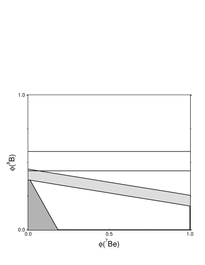
Figure 2: Neutrino fluxes observed in three experiments with the luminosity constraint of Eq. (25) imposed. The regions allowed by the Kamiokande (top), chlorine (middle) and gallium (bottom corner) are shown. For convenience the fluxes are normalized to the SSM values of Bahcall and Pinsonneault.

As we see in the next section the results from the solar neutrino experiments imply the existence of “new physics”, such as nonzero neutrino masses and mixing between the different kinds of neutrinos. Hence it is very important to test the reliability of these experiments. One such test is to expose these detectors to man-made neutrino sources with a known flux and energy. Both the GALLEX $\!{}^{{\bf?}}$ and SAGE $\!{}^{{\bf?}}$ collaborations recently reported results from such calibration experiments.

There are four criteria one needs to satisfy in choosing a portable neutrino source: (i) The mean energy of the neutrinos from the source must be close to the mean energy of the solar neutrinos detected at that particular detector; (ii) The activity should be such that test measurement reaches the precision of the solar neutrino measurement; (iii) The lifetime should be long enough so that the source can be transported from the production site to the detector without losing much strength; and (iv) There should be a reliable method to determine the source activity. A ${}^{51}Cr$ source satisfying these criteria was produced in Grenoble, and was used to expose the GALLEX detector. This was the strongest portable neutrino source ever produced, with an activity of $6.2\times 10^{16}$ decays per second. The ratio of the rate of ${}^{51}Cr$ produced neutrino signals to the rate expected from the known source activity was found to be $1.04\pm 0.12$, providing an overall check for the GALLEX detector and demonstrating the validity of the basic principles of radiochemical methods to detect these rare events (at a level of about 10 atoms per 30 tons of detector fluid). This result, with its 11% uncertainty, shows that the 40% deficit for the solar neutrino flux observed by GALLEX, as compared to the standard solar model expectation, is unlikely to be an experimental artifact. The SAGE collaboration similarly utilized a 93% enriched chromium source with an activity of $2\times 10^{16}$ decays per second. The irradiation of the enriched chromium was carried out at the fast neutron reactor in Aktau, Kazakhstan. At the start of the SAGE exposure, their initial source intensity was expected to produce about 14.7 germanium atoms a day as compared to the solar neutrino background of 0.3 atoms a day, about 50 times “brighter” than the sun. Their result for the ratio of the rate of source produced neutrino signal to the rate expected from the known source activity is $0.93\pm 0.15\pm 0.17$. This result also indicates that the deficit of solar neutrinos observed in the SAGE experiment is unlikely to be due to some instrumental problem in the experiment. Hence the results from GALLEX and SAGE both strongly support the notion of a real deficit of solar neutrinos below that predicted by the Standard Solar Models. These experiments in turn can be used to assess the excited state contributions to the ${}^{71}Ga$ neutrino capture cross-section $\!{}^{{\bf?}}$, and neutrino vacuum oscillations between the source and the detector $\!{}^{{\bf?}}$.

Earlier results from the Homestake experiment hinted a possibility of anti-correlation between solar neutrino counts and sunspot numbers. It is rather difficult to understand such a behavior in a theoretical framework. The most straightforward explanation for short-term time-variation of the neutrino flux is to assume the existence of a neutrino magnetic moment $\!{}^{{\bf?}}$. However, to obtain an anti-correlation of the observed amount, one needs rather large magnetic moments $\!{}^{{\bf?}}$, seemingly inconsistent with recent bounds obtained from stellar cooling rates for plasmon decay into neutrino-antineutrino pairs. $\!{}^{{\bf?}}$ (However neutrino magnetic moment could be important for supernova dynamics $\!{}^{{\bf?}}$). The present status of the neutrino magnetic moment solution to the solar neutrino problem is summarized in Ref. 41.

Solar neutrinos are not the only experimental probes of the sun. Information from helioseismological pulsation observations complement information obtained by solar neutrino experiments. The standing acoustic waves (p-waves) cause the solar surface to vibrate with a characteristic period of about five minutes. By observing red- and blue-shifts of patches of the solar surface, projecting them on spherical harmonics, and finally Fourier transforming with respect to the observation time one can obtain eigenfrequencies of the solar p-modes with great accuracy. For very high overtones (for a spherically-symmetric three-dimensional object such as the Sun these are characterized by two large integers), the equations describing p-modes simplify $\!{}^{{\bf?}}$ and one can reliably obtain a sound velocity profile for the outer half of the Sun using direct Abelian inversion. The sound density profile obtained this way agrees with the predictions of the standard solar model. By studying discontinuities in the sound velocity profile, it is also possible to reliably extract the location of the bottom of the convective zone $\!{}^{{\bf?}}$. More recent experimental developments made extensive helioseismic data available, including results from the GONG network $\!{}^{{\bf?}}$ and SOI/MDI project on the SOHO satellite $\!{}^{{\bf?}}$. These data include lower overtones that penetrate the solar core and make a direct inversion for the solar internal sound speed possible down to 0.05 R_⊙. Different standard solar models are generally in good agreement with the observations $\!{}^{{\bf?},{\bf?}}$.

3.3 Implications of the Data

Over the years various astrophysical solutions to explain the deficiency of the solar neutrinos were proposed. The model-independent argument given in the previous subsection and sketched in Figure 2 severely limits, but not necessarily eliminates, an astrophysical solution. One may attempt to lower the core temperature of the Sun, but in doing so both the ${}^{7}Be$ and ${}^{8}B$ neutrino fluxes are suppressed, contradicting the data $\!{}^{{\bf?}}$. Recently an alternative astrophysical solution was proposed $\!{}^{{\bf?}}$, namely slow mixing of the solar core on time scales characteristic of the ${}^{3}He$ equilibration discussed in Section 3.1. The basic idea here is to find a mechanism to bring ${}^{3}He$ from 0.2 R_⊙ to the inner core where the temperature is higher. Since after the ${}^{7}Be$ equilibrium is reached ${}^{7}Be$ equilibrium abundance follows ${}^{3}He$ abundance, ${}^{7}Be$ is then burned at the higher temperatures prevalent at $\sim 0.05R_{\odot}$. A high value of the temperature does not significantly change the rate of the electron-capture reaction $e^{-}+^{7}$Be$\rightarrow^{7}$Li$+\nu_{e}$, but exponentially enhances the rate of the reaction $p+^{7}$Be$\rightarrow^{8}$B$+\gamma$ where the first step is quantum mechanical tunneling. In fact the latter reaction is enhanced so much that it is necessary to reduce the core temperature from the Standard Solar Model value in the simple model Cumming and Haxton considered. Imposing such a lower temperature on the Standard Solar Model is ruled out by the helioseismological data $\!{}^{{\bf?}}$. Whether one can build a non-standard solar model along the ideas of Cumming and Haxton and still be consistent with the helioseismology needs to be further explored.

An alternative approach is to explain the deficiency with new neutrino physics, either using the MSW effect discussed in Section 2.2, or using the vacuum oscillations discussed in Section 2.1. During the last decade such analyses were given by many authors. Here we quote the most recent such analysis given by Hata and Langacker $\!{}^{{\bf?}}$. The parameter space allowed by the current data is shown in Figure 3 as calculated by them. The MSW solution currently seems to be the most-favored solution to the solar neutrino problem.

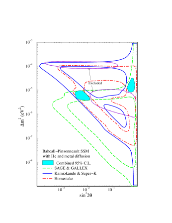
Figure 3: MSW parameter space (shaded regions) allowed by observations assuming Bahcall-Pinsonneault standard solar model with He diffusion as calculated by Hata and Langacker. Also shown are the regions excluded by the Kamioka day-night data.

3.4 Future Experiments

Neutrino oscillation solutions to the solar neutrino problem convert electron neutrinos into neutrinos of other flavors. Testing the MSW scenario requires detecting these other flavors. One experiment designed to achieve this goal is Sudbury Neutrino Observatory (SNO). The heavy water Cerenkov detector to be located at SNO is expected to have a sensitivity approximately 50 times that of the Homestake experiment $\!{}^{{\bf?}}$. The neutrinos are detected through the charged current reaction

$$\nu_{e}+d\rightarrow p+p+e^{-},$$ (27)

and the neutral current reactions

$$\nu_{e}+e^{-}\rightarrow\nu_{e}+e^{-},$$ (28)

$$\nu_{x}(\overline{\nu}_{x})+d\rightarrow\nu_{x}(\overline{\nu}_{x})+p+n.$$ (29)

The electron antineutrinos coming from a supernova or a possible spin-flavor precession in the Sun can also be detected through the reaction

$$\overline{\nu}_{e}+d\rightarrow n+n+e^{+}.$$ (30)

The produced neutrons will be detected either by using $(n,\gamma)$ reactions on nuclear targets or by using ${}^{3}He$ proportional counters. The electrons coming from the reaction in Eq. (27) are essentially monochromatic with energies $\sim E_{\nu}-1.44$ MeV and they have a very different angular distribution ($1-\cos\theta_{e}/3$) with respect to the neutrino direction than that of the electrons coming from the reaction in Eq. (28) (which are constrained to the forward cone). It will be possible to measure not only the total flux, but also the energy dependence of the neutrino flux at SNO. In addition to detecting solar neutrinos, SNO could be a useful tool in studying a galactic supernova $\!{}^{{\bf?}}$.

Another experiment currently under construction is BOREXINO $\!{}^{{\bf?}}$. which will observe neutrino electron scattering in an organic scintillator with a threshold of 250 keV. It will have the capability of measuring ${}^{7}Be$ neutrino flux and looking for seasonal flux variations due to vacuum oscillations and day/night effect. Furthermore BOREXINO has a good sensitivity to an antineutrino signal (about 20 ev/year). As mentioned above an antineutrino signal, not expected by the standard solar model, could be an indication of a neutrino magnetic moment $\!{}^{{\bf?}}$.

4 Atmospheric Neutrinos

Atmospheric neutrinos arise from the decay of secondary pions, kaons, and muons produced by the collisions of primary cosmic rays with the oxygen and nitrogen nuclei in the upper atmosphere. For energies less than 1 GeV all the secondaries decay :

Table 4: Ratio of Ratios, R of Eq. (33), as observed in different experiments.

Experiment	R
Kamioka $\!{}^{{\bf?}}$	$0.60\pm 0.06$
Superkamioka $\!{}^{{\bf?}}$	$0.67\pm 0.05\pm 0.06$
IMB $\!{}^{{\bf?}}$	$0.54\pm 0.05\pm 0.07$
Soudan 2 $\!{}^{{\bf?}}$	$0.72\pm 0.19\pm 0.07$
Nusex $\!{}^{{\bf?}}$	$1.0\pm 0.3$
Frejus $\!{}^{{\bf?}}$	$0.99\pm 0.13\pm 0.08$
Baksan $\!{}^{{\bf?}}$	$0.95\pm 0.22$

$$\pi^{\pm}(K^{\pm}) \rightarrow \mu^{\pm}+\nu_{\mu}(\overline{\nu}_{\mu}),$$

$$\mu^{\pm} \rightarrow e^{\pm}+\nu_{e}(\overline{\nu}_{e})+\overline{\nu}_{\mu}(\nu_{\mu}).$$ (31)

Consequently one expects the ratio

$$r=(\nu_{e}+\overline{\nu}_{e})/(\nu_{\mu}+\overline{\nu}_{\mu})$$ (32)

to be approximately 0.5 in this energy range. Detailed Monte Carlo calculations $\!{}^{{\bf?}}$, including the effects of muon polarization, give $r\sim 0.45$. Since one is evaluating a ratio of similarly calculated processes, systematic errors are significantly reduced. Different groups estimating this ratio, even though they start with neutrino fluxes which can differ in magnitude by up to 25%, all agree within a few percent $\!{}^{{\bf?}}$. The ratio (observed to predicted) of ratios

$$R={(\nu_{\mu}/\nu_{e})_{\rm data}\over(\nu_{\mu}/\nu_{e})_{\rm MonteCarlo}}$$ (33)

was determined in several experiments as summarized in Table 4. There seems to be a persistent discrepancy between theory and experiment. Neutrino oscillations are generally invoked to explain this discrepancy $\!{}^{{\bf?}}$.

Experimentally the ratio of ratios, $R$, appears to be independent of zenith angle. The observed zenith angle distribution of low energy atmospheric neutrinos is consistent with no oscillations or with a large number of oscillations for all source-detector distances. Explanations of the low energy atmospheric neutrino anomaly based on the oscillation of two neutrino flavors require that the oscillating term $\!{}^{{\bf?}}$, $\cos(\frac{\delta m^{2}L}{2E})$, average to zero for even the shortest source-detector distances ($L<50$ km for neutrinos from directly overhead.) For neutrinos in the energy range 0.1 to 1 GeV this condition is satisfied for $\delta m^{2}>10^{-3}eV^{2}$. If the atmospheric neutrino anomaly is resolved by the oscillations of muon into tau neutrinos, this value of $\delta m^{2}$ is consistent with a tau neutrino mass relevant to hot dark matter and supernova dynamics (cf. Section 5). It is also possible to make a search in the three-neutrino-flavor parameter space and identify regions in this parameter space compatible with the existing atmospheric and solar neutrino data within the vacuum oscillation scheme $\!{}^{{\bf?}}$.

5 Neutrino Flavor Mixing in Supernovae

Understanding neutrino transport in a supernova is an essential part of understanding supernova dynamics. Neutrino transport in a medium like supernova is a complicated process which needs to be treated numerically taking into account many different pieces of physics. In these lectures only the effects of neutrino flavor mixing on supernova dynamics are covered. In a core-collapse driven supernova, the inner core collapses subsonically, but the outer part of the core supersonically. At some point during the collapse, when the nuclear equation of state stiffens, the inner part of the core bounces, but the outer core continues falling in. The shock wave generated at the boundary loses its energy as it expands by dissociating material falling through it into free nucleons and alpha particles. For a large initial core mass, the shock wave gets stalled at $\sim$ 200 to 500 km away from the center of the proto-neutron star $\!{}^{{\bf?}}$. Meanwhile, the proto-neutron star, shrinking under its own gravity, loses energy by emitting neutrinos, which only interact weakly and can leak out on a relatively long diffusion time scale. The question to be investigated then is the possibility of regenerating the shock by neutrino heating.

Figure 4: Neutrinosphere and the stalled shock in a core-collapse driven supernova.

The situation at the onset of neutrino heating is depicted in Figure 4. The density at the neutrinosphere is $\sim 10^{12}$g cm^-3 and the density at the position of the stalled shock is $\!{}^{{\bf?}}$ $\sim 2\times 10^{7}$ g cm^-3. Writing the MSW resonance density in appropriate units:

$$\rho_{\rm res}=1.31\times 10^{7}\left({\delta m^{2}\over{\rm eV}^{2}}\right)\left({{\rm MeV}\over E_{\nu}}\right)\left({0.5\over{\rm Y}_{e}}\right){\rm g}\>{\rm cm}^{-3},$$ (34)

one sees that, for small mixing angles, $E_{\nu}\sim 10$ MeV, and cosmologically interesting $\delta m^{2}\sim 1-10^{4}$ eV², there is an MSW resonance point between the neutrinosphere and the stalled shock.

Most neutrinos emitted from the core are produced by a neutral current process, and so the luminosities are approximately the same for all flavors. The energy spectra are approximately Fermi-Dirac with a zero chemical potential characterized by a neutrinosphere temperature. The $\nu_{\tau},{\overline{\nu}}_{\tau},\nu_{\mu},{\overline{\nu}}_{\mu}$ interact with matter only via neutral current interactions. These decouple at relatively small radius and end up with somewhat high temperatures, about 8 MeV. The ${\overline{\nu}}_{e}$’s decouple at a larger radius because of the additional charged current interactions with the protons, and consequently have a somewhat lower temperature, about 5 MeV. Finally, since they undergo charged current interactions with more abundant neutrons, $\nu_{e}$’s decouple at the largest radius and end up with the lowest temperature, about 3.5 to 4 MeV. An MSW resonance between the neutrinosphere and the stalled shock can then transform $\nu_{\tau}\leftrightarrow\nu_{e}$, cooling $\nu_{\tau}$’s, but heating $\nu_{e}$’s. Since the interaction cross section of electron neutrinos with the matter in the stalled shock increases with increasing energy, it may be possible to regenerate the shock. Fuller et al. found that for small mixing angles between $\nu_{\tau}$ and $\nu_{e}$ one can get a 60% increase in the explosion energy $\!{}^{{\bf?}}$.

There is another implication of the $\nu_{\tau}$ and $\nu_{e}$ mixing in the supernovae. Supernovae are possible r-process sites $\!{}^{{\bf?}}$, which requires a neutron-rich environment, i.e., the ratio of electrons to baryons, $Y_{e}$, should be less than one half. $Y_{e}$ in the nucleosynthesis region is given approximately by $\!{}^{{\bf?}}$

$$Y_{e}\simeq{1\over 1+\lambda_{{\overline{\nu}}_{e}p}/\lambda_{\nu_{e}n}}\simeq{1\over 1+T_{{\overline{\nu}}_{e}}/T_{\nu_{e}}},$$ (35)

where $\lambda_{\nu_{e}n}$, etc. are the capture rates. Hence if $T_{{\overline{\nu}}_{e}}>T_{\nu_{e}}$, then the medium is neutron-rich. As we discussed above, without matter-enhanced neutrino oscillations, the neutrino temperatures satisfy the inequality $T_{\nu_{\tau}}>T_{{\overline{\nu}}_{e}}>T_{\nu_{e}}$. But the MSW effect, by heating $\nu_{e}$ and cooling $\nu_{\tau}$ can reverse the direction of inequality, making the medium proton-rich instead. Hence the existence of neutrino mass and mixings puts severe constraints on heavy-element nucleosynthesis in supernova. These constraints are investigated in Ref. 67.

6 Neutrino Propagation in Stochastic Media

In implementing the MSW solution to the solar neutrino problem one typically assumes that the electron density of the Sun is a monotonically decreasing function of the distance from the core and ignores potentially de-cohering effects $\!{}^{{\bf?}}$. To explore the validity of these assumptions parametric changes in the density and matter currents were considered $\!{}^{{\bf?}}$. More recently Loreti and Balantekin $\!{}^{{\bf?}}$ considered neutrino propagation in stochastic media. They studied the situation where the electron density in the medium has two components, one average component given by the Standard Solar Model or Supernova Model, etc. and one fluctuating component. Then the Hamiltonian in Eq. (7) takes the form

$$\hat{H}=\left({{-\delta m^{2}}\over 4E}\cos 2\theta+{1\over\sqrt{2}}G_{F}(N_{e}(r)+N^{r}_{e}(r))\right){\sigma_{z}}+\left({{\delta m^{2}}\over 4E}\sin 2\theta\right){\sigma_{x}}.$$ (36)

where one imposes for consistency

$$\langle N^{r}_{e}(r)\rangle=0,$$ (37)

and a two-body correlation function

$$\langle N^{r}_{e}(r)N^{r}_{e}(r^{\prime})\rangle={\beta}^{2}\ N_{e}(r)\ N_{e}(r^{\prime})\ \exp(-|r-r^{\prime}|/\tau_{c}),$$ (38)

where $\beta$ is a measure of the amount of the fluctuation, and $\tau_{c}$ is the correlation length. In the calculations of the Wisconsin group the fluctuations are typically taken to be subject to colored noise, i.e., higher order correlations

$$f_{12\cdots}=\langle N^{r}_{e}(r_{1})N^{r}_{e}(r_{2})\cdots\rangle$$ (39)

are taken to be zero for an odd number of $N^{r}_{e}$’s and

$$f_{1234}=f_{12}f_{34}+f_{13}f_{24}+f_{14}f_{23},$$ (40)

and its appropriate generalization for an even number of $N^{r}_{e}$’s.

Figure 5: Mean electron neutrino survival probability in the sun with fluctuations. The average electron density is given by the Standard Solar Model of Bahcall and Pinsonneault and $\sin^{2}2\theta=0.01$.

Mean survival probability for the electron neutrino in the Sun is shown in Figure 5 where fluctuations $\!{}^{{\bf?}}$ are imposed on the average solar electron density given by the Bahcall-Pinsonneault model. In this figure there are two salient features. The first one is that for very large fluctuations the MSW effect is “undone”. Complete flavor de-polarization is achieved, i.e. the neutrino survival probability is 0.5, the same as the vacuum oscillation probability for long distances. To illustrate this behavior the results from the physically unrealistic case of 50% fluctuations are shown. The second one is that the effect is largest when the neutrino propagation in the absence of fluctuations is adiabatic. This immediately suggests implementing this scenario to the neutrino conversion in a core-collapse supernova $\!{}^{{\bf?}}$ as described in Section 5. These conclusions were also confirmed by other authors. $\!{}^{{\bf?}}$${}^{\!-\,}$$\!{}^{{\bf?}}$ Propagation of a neutrino with a magnetic moment in a random magnetic moment has also been investigated. $\!{}^{{\bf?}}$^,$\!{}^{{\bf?}}$

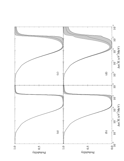
Figure 6: Mean electron neutrino survival probability plus minus $\sigma$ in the sun with fluctuations. The average electron density is given by the Standard Solar Model of Bahcall and Pinsonneault and $\sin^{2}2\theta=0.01$. Panels (a), (b), (c), and (d) correspond to an average fluctuation of 1%, 2%, 4%, and 8% respectively.

Using Eqs. (36) through (40), it is possible to calculate not only the mean survival probability, but also the variance, $\sigma$, of the fluctuations to get a feeling for the distribution of the survival probabilities. Results obtained for several representative cases are shown $\!{}^{{\bf?}}$ in Figure 6. This broadening of the survival probabilities may be measurable in real-time experiments sensitive to the low-energy component of the solar neutrino flux.

In these calculations the correlation length $\tau_{c}$ is taken to be very small, of the order of 10 km., to be consistent with the helioseismic deduction of the sound speed $\!{}^{{\bf?}}$. In the opposite limit of very large correlation lengths are very interesting result is obtained $\!{}^{{\bf?}}$, namely the averaged density matrix is given as an integral

$$\lim_{\tau_{c}\to\infty}\langle\hat{\rho}(r)\rangle={1\over{\sqrt{2\pi\beta^{2}}}}\int_{-\infty}^{\infty}dx\exp[{-x^{2}/(2\beta^{2})}]\hat{\rho}(r,x),$$ (41)

reminiscent of the channel-coupling problem of nuclear physics in the sudden limit. $\!{}^{{\bf?}}$

Finally we should mention that if the magnetic field in a polarized medium has a domain structure with different strength and direction in different domains, the modification of the potential felt by the neutrinos due polarized electrons will have a random character as depicted in Eq. (39) $\!{}^{{\bf?}}$.

References

References

- [1] http://www.hep.anl.gov/NDK/Hypertext/nuindustry.html.
- [2] http://neutrino.pc.helsinki.fi/neutrino/.
- [3] http://www.sns.ias.edu/j̃nb/.
- [4] http://dept.physics.upenn.edu/w̃ww/neutrino/solar.html.
- [5] P. LePage, contribution to these Proceedings.
- [6] See for example J.W.F. Valle, in Proceedings of Jorge Swieca Summer School on Nuclear Physics, Rio de Janeiro, Brazil, 1995 (hep-ph/9603307); J.W.F. Valle, hep-ph/9702231.
- [7] M. Gell-Mann, R. Slansky, and P. Ramond, in Supergravity, (North Holland, Amsterdam, 1979), p. 346; T. Yanagida, in Proceedings of the Workshop on Unified Theory and Baryon Number in the Universe, (KEK, Japan, 1979).
- [8] C. Athanassopoulos et al., Phys. Rev. Lett. 75, 2650 (1995).
- [9] J.E. Hill, Phys. Rev. Lett. 75, 2654 (1995).
- [10] B. Armbruster et al., Nucl. Phys. B (Proc. Suppl.) 38, 235 (1995).
- [11] C. Athanassopoulos et al., Phys. Rev. C54, 2685 (1996).
- [12] L. Wolfenstein, Phys. Rev. D 17, 2369 (1978); Phys. Rev. D 20, 2634 (1979).
- [13] S.P. Mikheyev and A. Yu. Smirnov, Sov. J. Nucl. Phys. 42, 913 (1985); Sov. Phys. JETP 64, 4 (1986).
- [14] H.A. Bethe, Phys. Rev. Lett. 56, 1305 (1986); S.P. Rosen and J.M. Gelb, Phys. Rev. D 34, 969 (1986); E.W. Kolb, M.S. Turner, and T.P. Walker, Phys. Lett. B 175, 478 (1986); V. Barger, K. Whisnant, S. Pakvasa, and R.J.N. Phillips, Phys. Rev. D 22, 2718 (1980); V. Barger, R.J.N. Phillips, and K. Whisnant, ibid. 34, 980 (1986).
- [15] W.C. Haxton, Phys. Rev. Lett. 57, 1271 (1986); S.J. Parke, Phys. Rev. Lett. 57, 1275 (1986).
- [16] A.B. Balantekin and J.F. Beacom, Phys. Rev. D 54, 6323 (1996).
- [17] A.B. Balantekin, S.H. Fricke, and P.J. Hatchell, Phys. Rev. D 38, 935 (1988).
- [18] E. Adelberger et al., Rev. Mod. Phys., in preparation.
- [19] J. N. Bahcall, Neutrino Astrophysics, (Cambridge University Press, Cambridge, 1989).
- [20] Solar Modeling, A.B. Balantekin and J.N. Bahcall, Eds., (World Scientific, Singapore, 1994).
- [21] R. Davis, D. S. Harmer, and K. C. Hoffman, Phys. Rev. Lett. 20, 1205 (1968); J. K. Rowley, B. T. Cleveland, and R. Davis in Solar Neutrinos and Neutrino Astronomy (Lead High School, South Dakota), Proceedings, edited by M. L. Cherry, K. Lande, and W. A. Fowler, AIP Conf. Proc. No. 126 (AIP, New York, 1985), p. 1.
- [22] K. S. Hirata et al., Phys. Rev. Lett. 63, 16 (1989); 65, 1297 (1990);65, 1301 (1990); 66, 9 (1991).
- [23] W. Hampel et al., Phys. Lett. B 388, 384 (1996).
- [24] J.N. Abdurashitov et al., Phys. Lett. B 328, 234 (1994); V.N. Gavrin, Proceedings of Neutrino 96, Ed. K. Enqvist, K. Huitu, and J. Maalampi, (World Scientific, Singapore, 1996).
- [25] For recent reviews see: W.C. Haxton, Ann. Rev. Astron. Astrophys. 33, 459, 1995; A.Yu. Smirnov, hep-ph/9611435.
- [26] K. Lande, Proceedings of Neutrino 96, Ed. K. Enqvist, K. Huitu, and J. Maalampi, (World Scientific, Singapore, 1996).
- [27] Y. Fukuda it et al., Phys. Rev. Lett. 77, 1683 (1996); Y. Suzuki, Proceedings of Neutrino 96, Ed. K. Enqvist, K. Huitu, and J. Maalampi, (World Scientific, Singapore, 1996).
- [28] Kenneth K. Young (for the Superkamiokande Collaboration), in http://www.phys.washington.edu/ỹoung/superk/drafts/ aps97.html.
- [29] J.N. Bahcall and M.H. Pinsonneault, Rev. Mod. Phys. 67, 781 (1995).
- [30] S. Turck-Chieze and I. Lopes, Astrophys. J. 408, 347 (1993).
- [31] M. Spiro and D. Vignaud, Phys. Lett. B 242, 279 (1990); N. Hata, S. Bludman, and P. Langacker, Phys. Rev. D 49, 3622 (1994); V. Castellani et al., Phys. Lett. B 324, 425 (1994); S. Parke, Phys. Rev. Lett. 74, 839 (1995); K.M. Heeger and R.G.H. Robertson, Phys. Rev. Lett. 77, 3720 (1996); V. Berezinsky, G. Fiorentini, and M. Lissia, Phys. Lett. B 365, 185 (1996).
- [32] J.N. Bahcall and P.I. Krastev, Phys. Rev. D 53, 4211 (1996).
- [33] P. Anselmann et al., Phys. Lett. B 342, 440 (1995).
- [34] J.N. Abdurashitov et al., Phys. Rev. Lett. 77, 4708 (1996).
- [35] N. Hata and W. Haxton, Phys. Lett. B 353, 422 (1995).
- [36] J. N. Bahcall, P. I. Krastev, E. Lisi, Phys. Lett. B 348, 121 (1995).
- [37] C.-S. Lim and W.J. Marciano, Phys. Rev. D 37, 1368 (1988), E. Kh. Akhmedov, Phys. Lett. B 213, 64 (1988).
- [38] A.B. Balantekin, P.J. Hatchell, and F. Loreti, Phys. Rev. D 41, 3583 (1990); A.B. Balantekin and F. Loreti, Phys. Rev. D 48, 5496 (1993).
- [39] G.E. Raffelt, Stars as Laboratories for Fundamental Physics : The Astrophysics of Neutrinos, Axions, and Other Weakly Interacting Particles, (University of Chicago Press, Chicago, 1996).
- [40] H. Nunokawa, Y.-Z. Qian, and G.M. Fuller, Phys. Rev. D 55, 3265 (1997).
- [41] E.Kh. Akhmedov, hep-ph/9705451.
- [42] D. Gough, Solar Phys. 100, 65 (1985); D.O. Gough and J. Toomre, Ann. Rev. Astron. Astrophys. 29, 62 (1991).
- [43] J. Christensen-Dalsgaard, D.O. Gough, and M.J. Thompson, Astrophys. J. 378, 413 (1991).
- [44] J.W. Harvey et al., Science 272, 1284 (1996).
- [45] P.H. Scherrer et al., Solar Phys. 162, 129 (1996).
- [46] S. Basu, J. Christensen-Dalsgaard, J. Schou, M.J. Thompson, and S. Tomczyk, Astrophys. J. 460, 1064 (1996); D. O. Gough et al., Science 272, 1296 (1996); O. Richard, S. Vauclair, C. Charbonnel, and W.A. Dziembowski, Astron. Astrophys. 312, 1000 (1996).
- [47] J.N. Bahcall, M.H. Pinsonneault, S. Basu, and J. Christensen-Dalsgaard, Phys. Rev. Lett. 78, 17 (1997).
- [48] S. Bludman, D. Kennedy, and P. Langacker, Phys. Rev. D 45, 1810 (1992); S. Bludman, N. Hata, D. Kennedy, and P. Langacker, Phys. Rev. D 47, 2220 (1993).
- [49] A. Cumming and W.C. Haxton, Phys. Rev. Lett. 77, 4286 (1996).
- [50] N. Hata and P. Langacker, hep-ph/9705339.
- [51] G. Aardsma et al., Phys. Lett. B 194, 321 (1987).
- [52] A.B. Balantekin and F. Loreti, Phys. Rev. D 45, 1059 (1992).
- [53] C. Arpasella et al., Nucl. Phys. B (Proc. Supp.)32, 149 (1993); G. Bellini, Nucl. Phys. B (Proc. Supp.)48, 363 (1996);
- [54] R.S. Raghavan, A.B. Balantekin, F. Loreti, A.J. Baltz, S. Pakvasa, and J. Pantaleone, Phys. Rev. D 44, 3786 (1991).
- [55] G. Barr, T.K. Gaisser, and T. Stanev, Phys. Rev. D 39, 3532 (1989); T.K. Gaisser, T. Stanev, and G. Barr, ibid. 38, 85 (1988).
- [56] H. Lee and S.A. Bludman, Phys. Rev. D 37, 122 (1988); E.V. Bugaev and V.A. Naumov, Phys. Lett. B 232, 391 (1989); M. Honda, K, Kasahara, K. Hidaka, and S. Midorikawa, Phys. Lett. B 248, 193 (1990); M. Kawasaki and S. Mizuta, Phys. Rev. D 43, 2900 (1991).
- [57] Y. Suzuki, in Proceedings of Neutrino 96, ed. K. Enqvist K. Huitu, and J. Maalampi, (World Scientific, Singapore, 1996).
- [58] R. Becker-Szendy, et al., Phys. Rev. D 46, 3720 (1992).
- [59] Quoted in Reference 2.
- [60] N. Aglietta, et al., Europhys. Lett. 8, 611 (1989).
- [61] Ch. Berger, et al., Phys. Lett. B 227, 489 (1989).
- [62] J.G. Learned, S. Pakvasa, and T. Weiler, Phys. Lett. B 207, 79 (1988); V. Barger and K. Whisnant, ibid. 209, 365 (1988); K. Hidaka, M. Honda, and S. Midorikawa, Phys. Lett. B 61, 1537 (1988).
- [63] S.M. Bilenky and S.T. Petcov, Rev. Mod. Phys. 59, 671 (1987).
- [64] A. Acker, A.B. Balantekin, and F.N. Loreti, Phys. Rev. D 49, 328 (1994).
- [65] G.M. Fuller, R.W. Mayle, B.S. Meyer, and J.R. Wilson, Astrophys. J. 389, 517 (1992); R.W. Mayle, in Supernovae, A.G. Petschek, Ed., (Springer-Verlag, New York, 1990).
- [66] E.M. Burbidge, G.R. Burbidge, W.A. Fowler, and F. Hoyle, Rev. Mod. Phys. 29, 694 (1957).
- [67] Y.Z. Qian, G.M. Fuller, G.J. Mathews, R.W. Mayle, J.R. Wilson, and S.E. Woosley, Phys. Rev. Lett. 71, 1965 (1993).
- [68] R.F. Sawyer, Phys. Rev. D 42, 3908 (1990).
- [69] A. Halprin, Phys. Rev. D 34, 3462 (1986); A. Schafer and S.E. Koonin, Phys. Lett. B 185, 417 (1987); P. Krastev and A.Yu. Smirnov, Phys. Lett. B 226, 341 (1989), Mod. Phys. Lett. A6, 1001 (1991); W. Haxton and W.M. Zhang, Phys. Rev. D 43, 2484 (1991).
- [70] F.N. Loreti and A.B. Balantekin, Phys. Rev. D 50, 4762 (1994).
- [71] A.B. Balantekin, J. M. Fetter, and F. N. Loreti, Phys. Rev. D 54, 3941 (1996).
- [72] F.N. Loreti, Y.Z. Qian, G.M. Fuller, A.B. Balantekin, Phys. Rev. D 52, 6664 (1995).
- [73] H. Nunokawa, A. Rossi, V.B. Semikoz, and J.W.F. Valle, Nucl. Phys. B 472, 495 (1996); J.W.F. Valle, Nucl. Phys. Proc. Suppl. 48, 137 (1996); A. Rossi, ibid., 384 (1996).
- [74] C.P. Burgess and D. Michaud, Ann. Phys., 256, 1 (1997).
- [75] E. Torrente-Lujan, hep-ph/9602398.
- [76] S. Pastor, V.B. Semikoz, J.W.F. Valle, Phys. Lett. B 369, 301 (1996).
- [77] A.B. Balantekin and N. Takigawa, Ann. Phys.160, 441 (1985).
- [78] H. Nunokawa, V.B. Semikoz, A.Yu. Smirnov, and J.W.F. Valle, hep-ph/9701420.