The supermassive black hole of M87 and the kinematics of its associated gaseous disk

Abstract

We have obtained long-slit observations of the circumnuclear region of M87 at three different locations, with a spatial sampling of 0$\farcs$028 using the Faint Object Camera f/48 spectrograph on board HST. These data allow us to determine the rotation curve of the inner $\sim$ 1″ of the ionized gas disk in $[{\rm O\,II}]$$\lambda$3727 to a distance as close as 0$\farcs$07 ($\simeq 5$pc) to the dynamic center, thereby significantly improving on both the spatial resolution and coverage of previous FOS observations. We have modeled the kinematics of the gas under the assumption of the existence of both a central black hole and an extended central mass distribution, taking into account the effects of the instrumental PSF, the intrinsic luminosity distribution of the line, and the finite size of the slit. We find that the central mass must be concentrated within a sphere whose maximum radius is 0$\farcs$05 ($\simeq$3.5pc) and show that both the observed rotation curve and line profiles are consistent with a thin–disk in keplerian motion. We conclude that the most likely explanation for the observed motions is the presence of a supermassive black hole and derive a value of $M_{BH}=(3.2\pm 0.9)\mbox{$\times 10^{9}$}$$\rm M_{\odot}$ for its mass.

1 Introduction

The presence of massive black holes at the center of galaxies is widely believed to be the common origin of the phenomena associated with so-called Active Galactic Nuclei. The black hole model is very appealing because it provides an efficient mechanism that converts gravitational energy, via accretion, into radiation within a very small volume as required by the rapid variability of the large energy output of AGN (e.g. Blandford (1991)).

The standard model comprises a central black hole with mass in the range $\simeq\mbox{$10^{6}$}-\mbox{$10^{9}$}\mbox{$\rm M_{\odot}$}$ surrounded by an accretion disk which releases gravitational energy. The radiation is emitted thermally at the local black–body temperature and is identified with the “blue–bump”, which accounts for the majority of the bolometric luminosity in the AGNs. The disk possesses an active corona, where infrared synchrotron radiation is emitted along with thermal bremsstrahlung X-rays. The host galaxy supplies this disk with gas at a rate that reflects its star formation history and, possibly, its overall mass (Magorrian et al. (1996)) thereby accounting for the observed luminosity evolution. Broad emission lines originate homogeneously in small gas clouds of density $\simeq\mbox{$10^{9}$}\mbox{$\rm cm^{-3}$}$ and size $\simeq$1 AU in random virial orbits about the central continuum source. Plasma jets are emitted perpendicular to the disk. At large radii, the material forms an obscuring torus of cold molecular gas. Orientation effects of this torus to the line-of-sight naturally account for the differences between some of the different classes of AGN (see Antonucci (1995) for a review). While this broad picture has been supported and refined by a number of observations, direct evidence for the existence of accretion disks around supermassive black holes is sparse (see, however, Livio and Xu, (1997)) and detailed measurements of their physical characteristics are conspicuous by their absence.

The giant elliptical galaxy M87 at the center of the Virgo cluster, at a red-shift of 0.0043 (de Vaucouleurs et al. (1991)), is well known for its spectacular, apparently one–sided jet, and has been studied extensively across the electromagnetic spectrum. Ground–based observations first revealed the presence of a cusp–like region in its radial light profile accompanied by a rapid rise in the stellar velocity dispersion and led to the suggestion that it contained a massive black hole (Young et al., (1978), Sargent et al., (1978)). Stellar dynamical models of elliptical galaxies showed however that these velocity dispersion rises did not necessarily imply the presence of a black hole, but could instead be a consequence of an anisotropic velocity dispersion tensor in the central 100pc of a triaxial elliptical potential (e.g. Duncan & Wheeler (1980), Binney and Mamon (1982)). Considerable controversy has surrounded this and numerous other attempts to verify the existence of the black hole in M87 and other nearby giant ellipticals using ground based stellar dynamical studies (e.g. Dressler and Richstone (1990), van der Marel (1994)). To-date the best available data remains ambiguous largely because of the difficulty of detecting the high-velocity wings on the absorption lines which are the hallmark of the black hole.

One of the major goals of HST has been to establish or refute the existence of black holes in active galaxies by probing the dynamics of AGN at much smaller radii than can be achieved from the ground.

HST emission line imagery (Crane et al. (1993), Ford et al., (1994)) of M87 has lead to the discovery of a small scale disk of ionized gas surrounding its nucleus which is oriented approximately perpendicularly to the synchrotron jet. This disk is also observed in both the optical and UV continuum (Macchetto 1996a and 1996b). Similar gaseous disks have also been found in the nuclei of a number of other massive galaxies (Ferrarese et al., (1994), Jaffe et al., (1994)).

Because of surface brightness limitations on stellar dynamical studies at HST resolutions, the kinematics of such disks are in practice likely to be the only way to determine if a central black hole exists in all but the very nearest galaxies. In the case of M87 FOS observations at two locations on opposite sides of the nucleus separated by 0$\farcs$5 showed a velocity difference of $\simeq$1000 km s^-1, a clear indication of rapid motions close to the nucleus (Harms et al., (1994)). By assuming that the gas kinematics determined at these and two additional locations arise in a thin rotating keplerian disk, Ford et al. (1996) estimated the central mass of M87 is $\simeq$2$\times 10^{9}$$\rm M_{\odot}$ with a range of variation between 1 and 3.5$\times 10^{9}$$\rm M_{\odot}$. Currently this result provides the most convincing observational evidence in favour of the black hole model. Implicit in this measurement of the mass of the central object, however, is the assumption that the gas motions in the innermost regions reflect keplerian rotation and not the effects of non gravitational forces such as interactions with the jet. Establishing the detailed kinematics of the disk is therefore vital.

In this paper we present new FOC,f/48 long-slit spectroscopic observations of the ionized circumnuclear disk of M87 with a pixel size of 0$\farcs$028. They provide us with a $[{\rm O\,II}]$$\lambda$3727 rotation curve in three different locations on the disk and which extend up to a distance of $\sim$ 1″. We show that the observations are consistent with a thin–disk in keplerian motion, which explains the observed rotation curve and line profiles, and we derive a mass of $M_{BH}=(3.2\pm 0.9)\mbox{$\times 10^{9}$}$$\rm M_{\odot}$ within a radius of $\simeq$5pc for the central black hole.

The plan of the paper is as follows: the observations and data reduction are described in sections 2 and 3. In section 4 we use the current data and previous HST images to constrain the precise location of the slit with respect to the nucleus of M87. The results of the observations are presented in section 5 and compared to HST/FOS observations in section 6. In section 7 and 8 we discuss the fitting procedures to the observed rotation curve and line profiles with increasingly sophisticated models and in section 9 we compare the observed line profiles with the predictions from the keplerian model of a thin disk. Limits on the distributed mass are discussed in section 10 and the conclusions are given in section 11.

Following Harms et al., (1994) we adopt a distance to M87 of 15 Mpc throughout this paper, whence 0$\farcs$1 correspond to 7.3 pc.

2 Observations

The circumnuclear disk of M87 was observed using the Faint Object Camera f/48 long–slit spectrograph on board the Hubble Space Telescope on July 25^th, 1996 at resolutions of 1.78Å and 0$\farcs$0287 per pixel along the dispersion and slit directions, respectively. The F305LP filter was used to isolate the first order spectrum which covers the 3650–5470 Å region and therefore includes the $[{\rm O\,II}]$$\lambda$3727, H$\beta$$\lambda$4861 and $[{\rm O\,III}]$$\lambda$$\lambda$4959, 5007 Å  emission lines. An interactive acquisition (integration time 297s) 1024x512 zoomed image was obtained with the f/48 camera through the F140W filter to accurately locate the nucleus. The slit, 0$\farcs$063x13$\farcs$5 in size, was positioned on the gas disk at a position angle of 47.3^∘ and initially spectra with exposure times of 2169 seconds were taken in the 1024x512 non–zoomed mode at 3 locations separated by 0$\farcs$2 centered approximately on the nucleus. These observations were used to derive the actual location of the nucleus and HST was then repositioned using a small angle maneuver to this location (which actually turned out to be virtually coincident with the position of the second of the three scans). This allowed us to position the slit to within 0$\farcs$1 of the nucleus (see section 4). A further higher signal-to-noise spectrum at this location was then obtained with a total exposure time of 7791 seconds, built from 3 shorter exposures, 2597 seconds in duration. The accuracy of the HST small angle maneuvers is known to be a few milliarcseconds and this is in agreement with the close correspondence between the four spectra taken on the nucleus during the spatial scan.

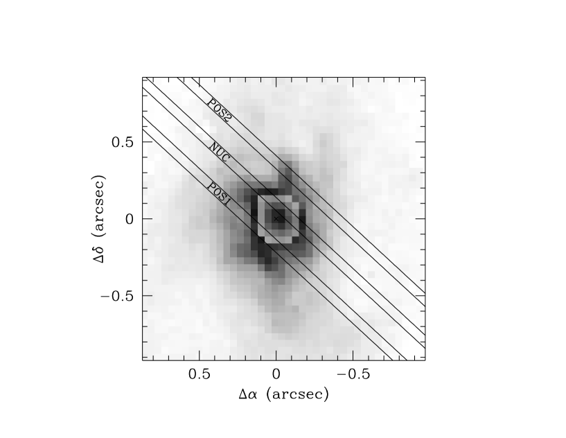
Figure 1: Positions of the slit during the observations compared with the H$\alpha$+$[{\rm N\,II}]$ image of the M87 disk from the WFPC2 archive. The gray levels are between 0 and 40% of the nuclear peak in the outer region. The nucleus has been rescaled to be displayed within this range of values. North is up and east is to the left.

The actual slit positions, as derived in section 4, are displayed in Fig. 1 superposed on the H$\alpha$+$[{\rm N\,II}]$ image published by Ford et al., (1994) which we retrieved from the HST archive. Hereafter we will refer to them as POS1, NUC and POS2 from South–East to North–West, respectively. In Tab. 1 we list the datasets obtained for M87 and those which were used for the calibration.

3 Data reduction

The raw FOC data suffer from geometric distortion, i.e., the spatial relations between objects on the sky are not preserved in the raw images produced by the FOC cameras. This geometric distortion can be viewed as originating from two distinct sources. The first of these, optical distortion, is external to the detectors and arises because of the off–axis nature of the instrument aperture. The second, and more significant source of distortion is the detector itself, which is magnetically focused.

All frames, including those used for calibration, were geometrically corrected using the equally spaced grid of reseau marks which is etched onto the first of the bi–alkali photocatodes in the intensifier tube (Nota, Jedrzejewski & Hack, (1995)). This geometric correction takes into account both the external and internal distortions. The positions of the reseau marks were measured on each of the internal flat–field frames which were interspersed between the spectra. The transformation between these positions and an equally spaced 9x17 artificial grid was then computed by fitting bi-dimensional Chebyshev polynomials of 6^th order in x and y terms and 5^th order in the cross terms. This transformation was applied to the science images resulting in a mean uncertainty in the reseau position of 0.10–0.25 pixels, depending on the signal-to-noise (SNR) of the flat frames.

In addition, geometric distortion is also induced on the slit and dispersion directions by the spectrographic mirror and the grating. The distortion in the dispersion direction was determined by tracing the spectra of two stars taken in the core of the 47 Tucanae globular cluster. These stars are $\simeq$ 130 pixels apart and almost at the opposite extremes of the slit. The distortion along the slit direction was determined by tracing the brightness distribution along the slit of the planetary nebula NGC 6543 emission lines. Ground–based observations (Perez, Cuesta, Axon and Robinson, in preparation) indicate that the distortion induced by the velocity field of the planetary nebula are negligible (less than 0.5 Å) at the f/48 resolution. After rectification the spectra of the 47 Tuc stars and that of NGC 6543 were straight to better than 0.2 pixels on both axes. The wavelength calibration was determined from the geometrically corrected NGC 6543 spectrum. The reference wavelengths were again derived from the ground–based observations. The residual uncertainty on the wavelength calibration is less than 0.2Å. As a result of these procedures we obtained images with the dispersion direction along columns and the slit direction along rows. The pixel sizes are 0$\farcs$0287 in the spatial direction and 1.78Å along the dispersion direction.

The relatively small width of the lines of NGC 6543 (FWHM$<$ 100 km s^-1) allows us to estimate the instrumental broadening to be $\simeq$ 430$\pm$30 km s^-1. From the luminosity profile of the 47 Tuc stellar spectra the instrumental broadening along the spatial direction is 0$\farcs$08$\pm$0$\farcs$02.

The contributions to the total error budget from the various calibration steps can be summarized as follows:

• geometric correction with the reseau marks has a residual error of 0.10–0.25 pixels;

• rectification of the dispersion direction has a residual error less than 0.2 pixels;

• rectification along the slit direction has a residual error of 0.2 pixels;

• the error due to the intrinsic distortions of the planetary nebula velocity field is less than 0.5Å, i.e. 0.3 pixels;

• the residual error in the wavelength calibration is less than 0.15Å.

Combining all the uncertainty terms in quadrature we estimate a maximum uncertainty of 0.45 pixels (0.8 Å  which correspond to 65 km s^-1 at 3727 Å) and 0.28 pixels (8 mas) in the dispersion and spatial directions respectively. Moreover, when we restrict ourselves to a small region of the detector, corresponding to a single spectral line, both uncertainties are negligible compared to those arising from the SNR of the data.

The distortion correction and wavelength calibration were applied to the geometrically corrected M87 spectra and, as a check on our error budget, we traced the nuclear continuum emission. We found that the continuum was straight to better than 1 pixels across the whole spectral range and 0.5 pixels if we excluded the low SNR region of the spectrum redward of 4800 Å which was not used in our analysis.

The imperfect repositioning of the spectrographic mirror, which moves between flat–field and source exposures, caused shifts between successive spectra in both the spatial and spectral directions. By comparing the internal consistency of the four independent spectra of the nucleus of M87 we have determined that these shifts range from 1 to 4 pixels in the spatial direction and are less than 2 pixels in the dispersion direction. The four spectra were aligned to an accuracy of 0.02 pixels by cross-correlating the flux distribution of the $[{\rm O\,II}]$ line and co–added. The relative zero points of the other slit positions cannot be determined because the continuum is too weak to be detected. In the following analysis we will therefore conservatively allow for zero–point shifts in both the spatial and velocity directions of up to 4 pixels.

The background emission was subtracted in all the spectra by means of a spline fit along the slit direction after masking out the regions where line or continuum emission is detected. Similarly the continuum under the lines was subtracted with a first order polynomial fit along the dispersion direction.

4 Determination of the slit location

Given the 0$\farcs$2 step of the spatial scan and the slit width of 0$\farcs$063, the “impact parameter”, $b$, the minimum distance between the center of the slit and the nucleus is constrained to be smaller than 0$\farcs$1 by our observing strategy . We accurately determine $b$ by comparing the flux measured from each of our three slit positions with the brightness profile derived from a previous FOC,f/96 HST image in the F342W. This filter covers a similar spectral range and includes the dominant (Sec.5) line in our spectra, $[{\rm O\,II}]$. The F342W filter has a width of about 670 Å and the scale of the f/48 spectra along the dispersion direction is 1.78 Å/pixels. To correctly synthesize the spectral energy distribution transmitted by the F342W filter, for each slit we collapsed 376 spectral channels around the $[{\rm O\,II}]$ line and then measured the flux by co–adding 30 pixels (0$\farcs$9) around the peak in the slit direction.

A section of the F342W image, 0$\farcs$9 wide and parallel to the slit orientation was extracted. Since the continuum flux measured in our spectra is the spatial average over the slit width, we filtered the extracted f/96 image with a flat-topped rectangular kernel 0$\farcs$063 wide in the direction perpendicular to the slit. Leaving aside for the moment the different point-spread-functions (PSF) of the f/48 and f/96, the resulting brightness profile can be directly compared with the relative fluxes obtained from our spectroscopic measurements (as shown in Fig. 2). The value of the impact parameter which best reproduces the ratio of the fluxes measured in the three slit positions was determined from a least–squares fit to synthetic flux profile derived from the filter observation. As shown in Fig. 2 $\chi^{2}$ has one well defined minimum at $b=0\farcs 07\pm 0\farcs 01$.

To take into account the possible effects of the different PSFs for f/48 and f/96 we degraded the F342W image to the f/48 resolution. Since the f/96 and f/48 PSFs can be approximated by gaussians with FWHM 0$\farcs$04 and 0$\farcs$08 respectively, we convolved the f/96 image using a circularly symmetric gaussian function with a 0$\farcs$07 FWHM and repeated the analysis. As before the $\chi^{2}$ minimum falls at $0\farcs 07\pm 0\farcs 01$ implying that the different PSFs do not significantly affect the derived impact parameter. The positions of the slits with the impact parameter derived above are displayed in Fig. 1, overlayed on the H$\alpha$+$[{\rm N\,II}]$ continuum subtracted archival WFPC2 image .

5 Results

Extended $[{\rm O\,II}]$$\lambda$$\lambda$3726,3729 emission was detected in all three slit positions and the gray–scale, continuum subtracted $[{\rm O\,II}]$ image at NUC is displayed in Fig. 3.

At NUC we also detected $[{\rm S\,II}]$$\lambda$$\lambda$4076,4069 Å, $[{\rm O\,III}]$$\lambda$$\lambda$4959,5007 and possibly H$\beta$ emission. Since the $[{\rm O\,III}]$ lines fall close to a defect in the image, only the $[{\rm O\,II}]$ and $[{\rm S\,II}]$ were chosen as being suitable for velocity measurements.

The continuum subtracted lines were fitted, row by row, along the dispersion direction with single gaussian profiles using the task LONGSLIT in the TWODSPEC FIGARO package (Wilkins & Axon (1992)). In a few cases, at the edges of the emission region where the signal–to–noise ratio was insufficient, the fitting was improved by co-adding two or more pixels along the slit direction. All fits and respective residuals for the $[{\rm O\,II}]$ and $[{\rm S\,II}]$ lines can be found in Fig. 4. In all cases the measured line profiles are well represented by a single gaussian and constant continuum.

The resulting central velocities, FWHM’s and line intensities along the slit are plotted in Fig. 5 for the NUC position, and in Fig. 6 for POS1 and POS2. The corresponding continuum distribution along the slit is also shown in Fig. 5. Within the uncertainties, the velocities derived from $[{\rm S\,II}]$ (thin crosses) agree with those obtained from $[{\rm O\,II}]$ (filled squares), confirming the integrity of the wavelength calibration. The overall NUC velocity distribution indicates rotation with an amplitude of 1200 km s^-1, with a steep quasi–linear central portion between $\pm 0\farcs 2$ of the continuum peak and flattening at larger radii. Because of the much reduced signal–to–noise of POS1 and POS2 we primarily see only the brightest linear parts of the rotation curves but we do detect a clear turn–over to the South–West of POS1 at an amplitude of about 1000 km s^-1.

The line intensity profile at NUC increases steeply toward the center but is essentially flat-topped within the central 0$\farcs$14. The width of the lines at the three slit positions is significantly larger than the instrumental broadening (Fig. 4), even after taking into account the effects of density variations on the wavelengths of the density sensitive doublets (see the discussion below). Furthermore we note that at NUC the FWHM and the continuum peak are shifted by $\simeq$ 0$\farcs$06 ($\simeq$ 2 pixels). The significance of both these results will be discussed in Sec. 9.

The position–velocity diagram of the continuum subtracted $[{\rm O\,II}]$ line observed at NUC (Fig. 3) reveals the presence of two emission peaks $\simeq 800$ km/sec apart in velocity, spatially separated by approximately 0$\farcs$14. The existence of these two peaks implies that the line–emission does not increase monotonically to zero radius but rather that, at a certain distance smaller than 0$\farcs$07 from the nucleus ($\simeq 5$pc), the $[{\rm O\,II}]$ emission is absent.

5.1 The impact of density variations

One potential concern for the accuracy of the derived rotation curve is that the observed $[{\rm O\,II}]$ line is actually a blend of $[{\rm O\,II}]$$\lambda$3726.0 and $[{\rm O\,II}]$$\lambda$3728.8 i.e. they are separated by 225 km s^-1. We have adopted a central wavelength of 3727.15 Å in our analysis. However the doublet is density sensitive and it is important to determine the magnitude of the shift in the central wavelength of the doublet in response to density variations. Using a code kindly provided by Dr. E. Oliva, we computed the line emissivities for the $[{\rm O\,II}]$ lines using a five level atom and atomic parameters from a compilation by Mendoza (1983). As can be seen in Fig. 7, the ratio between the two lines varies between 0.68 (low density limit $N_{\rm e}$$<$ 50$\rm cm^{-3}$) to 2.88 (high density limit $N_{\rm e}$$>$$10^{5}$$\rm cm^{-3}$) and, consequently, any density–induced velocity shift is less than $\pm$ 45 km s^-1. Furthermore, from the archive FOS spectra described below (Sec. 6), the density derived from $[{\rm S\,II}]$$\lambda$6716/$\lambda$6731 ranges from $\simeq$ 200 to $\simeq$ 4300 $\rm cm^{-3}$ and this restricts the range of variation to $\pm$ 25 km s^-1. Similarly, the presence of an unresolved doublet will affect the measurements of the line widths. The greatest effect is when the lines are narrowest, i.e. when their FWHM is greater/equal to the instrumental broadening ($\simeq$ 430 km s^-1). In that case the FWHM of the $[{\rm O\,II}]$ doublet can be $\simeq$100 km s^-1 broader than that of a single line. When the FWHM is larger than 600 km s^-1 the broadening is less than 60 km s^-1 i.e. negligible for our data (Fig. 7).

We applied a similar treatment to the density sensitive $[{\rm S\,II}]$ doublet (Fig. 7) deriving a central wavelength of 4070.2 Å with a range of variation of $\pm$ 25 km s^-1 (atomic data from Cai and Pradhan (1993)). If, as the above density measurements imply, we are in the low density limit for the $\lambda$4076/$\lambda$4069 doublet then the central wavelength would be shifted to 4070.5 Å, implying an uncertainty of at most 25 km s^-1 in our assumed rest wavelength. We conclude that the variations induced by density effects are always within our measurement uncertainties.

6 Comparison with archival FOS observations

We retrieved the FOS data used by Harms et al., (1994) and Ford et al. (1996) from the HST archive. The datasets used and the corresponding target names are listed in Table 2, according to their notation, and their positions are compared with those of our slits in Fig. 8.

Because the FOS data are rather noisy we smoothed them by convolution with a 1.8Å–sigma gaussian, i.e. the FOS spectral resolution, and then measured the velocities of H$\beta$, $[{\rm O\,III}]$ $[{\rm O\,I}]$, H$\alpha$, $[{\rm N\,II}]$ and $[{\rm S\,II}]$ using single–gaussian fits as shown in Fig. 9. When possible H$\beta$ and the two $[{\rm O\,III}]$ lines were fitted simultaneously under the constraint that they had the same FWHM. In some cases it was also possible to satisfactorily deblend H$\alpha$, $[{\rm N\,II}]$ and the $[{\rm S\,II}]$ doublet. The measured ratio of the $[{\rm S\,II}]$ doublet implies an electron density which varies between 200 $\rm cm^{-3}$ and 4300 $\rm cm^{-3}$. The measured velocities are given in Table 3 and are in acceptable agreement with the values given in Table 1 of Harms et al., (1994). The similarity between the velocities obtained from different ionic species indicates that our results are not unduly biased by variations in the ionization conditions in the disk.

In Fig. 10 we compare the velocities obtained from our slit position NUC with those obtained from the FOS at POS4 through 6, in the 0$\farcs$26 aperture and at POS9 through 11, in the smaller 0$\farcs$09 aperture. The plotted uncertainties of the FOS data, typically between 50 and 100 km s^-1 in a given dataset, are the internal scatter of the velocities measured in a given aperture. Within the substantially larger uncertainties, the FOS rotation curve is in reasonable accord with our results. It is also clear that our data represent a considerable improvement in both spatial resolution and accuracy in the determination of the rotation curve of the disk.

7 Modeling the rotation curve: a simple but constructive approximation

We now derive the expected velocity measured along the slit for a thin disk in keplerian motion in a gravitational potential dominated by a condensed central source. At this stage we ignore both the finite width of the slit and effects of the PSF which will be considered in the next section. Although the limitations of this approximation are clear, since the angular scale of the region of interest is similar to the size of point–spread–function, several general conclusions can be drawn from this simplified treatment which clarify the behaviour or the more realistic model fits described in Sec. 8. For simplicity we will also refer to the condensed central source as a black hole deferring the reality of this assumption to Sec. 10.

Any given point $P$, located on the disk at a radius $R$, has a keplerian velocity

$$V(R)=\left(\frac{GM_{BH}}{R}\right)^{\frac{1}{2}}$$ (1)

where $M_{BH}$ is the mass of the black hole.

We choose a reference frame such that the X and Y axis, as seen on the plane of the sky, are along the major and minor axis of the disk respectively (see Fig. 11). In this coordinate system a point $P(X,Y)$ is at a radius $R$ such that

$$X^{2}+\frac{Y^{2}}{(\cos i)^{2}}=R^{2}$$ (2)

Each point along the slit can be identified by its distance s to the “center” of the slit O, whose distance from the nucleus defines the “impact parameter” $b$. Let $\theta$ be the angle between the slit and the major axis of the disk, i.e. the line of nodes, and define $i$ to be the inclination of the disk with respect to the line of sight. Since $P(X,Y)$ is located on the slit, X and Y are given by

$$X=-b\sin\theta+s\cos\theta\\$$ (3)

$$Y=b\cos\theta+s\sin\theta\\$$ (4)

The circular velocity $V(R)$ is directed tangentially to the disk as in Fig. 11 and its projection along the line of sight is then $-V(R)\cos\alpha\sin i$ (the - sign is to take into account the convention according to which blue–shifts result in negative velocities).

Making the transformation between coordinates on the plane of the disk and the X,Y on the plane of the sky

$$\tan\alpha=\frac{Y}{X\cos i}$$ (5)

hence, if $V_{sys}$ is the systemic velocity, the observed velocity along the slit is given by

$$V=V_{sys}-(GM_{BH})^{\frac{1}{2}}\frac{(\sin i)\,X}{\left(X^{2}+\frac{Y^{2}}{(\cos i)^{2}}\right)^{\frac{3}{4}}}$$ (6)

A non–linear least squares fit of the model defined in the equation 6, with $M_{BH}(\sin i)^{2}$, $\theta$, $i$, $b$, $V_{sys}$ and $cpix$ (which defines the origin of the $s$ axis) as free parameters to the observed rotation curve was obtained using simplex optimization code. Since the error bars on the independent variable are not negligible, we took them into account by minimizing the modified norm:

$$\chi^{2}=\sum_{i=1}^{N}\frac{\left(y_{i}-V(x_{i};p_{1},...,p_{6})\right)^{2}}{\Delta y_{i}^{2}+\left(\frac{\partial V}{\partial x}\right)_{x_{i}}^{2}\Delta x_{i}^{2}}$$ (7)

where $y_{i}$ is the measured velocity at the pixel $x_{i}$, there are $N$ data points and $p_{i}$ are the free parameters of the fit.

Because of the complexity of the fitting function we also carried out many trial minimizations using different initial estimates for the most critical free parameters, i.e. $i$, $\theta$ and $b$, taken from a large grid of several hundred, evenly spaced values. Many local minima of the $\chi^{2}$ function were found and we only accepted those solutions with a reduced $\chi^{2}<2.5$ and an impact parameter, $b$, consistent with that determined in Sec. 4 ($0\farcs 06<b<0\farcs 08$).

Even though there is considerable non–axisymmetric structure in the data, in their original analysis Harms et al., (1994) used a value for the inclination, $i=42^{\circ}\pm 5$, determined from isophotal fits to the surface photometry of the disk at radii ranging between 0$\farcs$3 and 0$\farcs$8 from the nucleus. Unfortunately, from our analysis of the imaging data it is not clear whether this result, obtained on the large scale, is valid at small radii (the inner 0$\farcs$3). To determine the inclination on the basis of surface photometry of the emission lines, higher spatial resolution images are needed and this can only be accomplished by HST measurements at UV wavelengths. Even then the bright non–thermal nucleus may dominate the structure of the central region. Indeed from our analysis of the kinematics the inclination is the most poorly constrained parameter, with acceptable values ranging from 47^∘ to 65^∘. Though the other parameters are intrinsically rather well constrained, in Table 4 we therefore show the variation of their allowed values for two inclination ranges.

A few points are evident from this analysis: the small angle $\theta$ to the line of nodes ($-5^{\circ}<\theta<4^{\circ}$) is a consequence of the apparent symmetry of the two branches of the rotation curve. When the impact parameter is non–null this symmetry can be achieved only if the slit direction is close to that of the line of nodes. The center of the rotation curve (between pixels 22.6 and 22.9) is close to the peak of the continuum distribution along the slit (pixels $\simeq$23–24) as one would expect if the latter indicates the location closest to the nucleus. However one would also expect the point with largest FWHM (pixel 25) to be coincident with it and not to be shifted by $\simeq$ 2 pixels ($\simeq 0\farcs 06$), as observed. We will return to this issue in the following sections. The systemic velocity is in reasonable agreement with the estimate of 1277 km s^-1 determined by van der Marel (1994) when one takes into account the uncertainty on the zero point of the wavelength calibration.

The two fits which have the minimum and maximum of the acceptable $\chi^{2}$ values are shown in Fig. 12 as solid and dotted lines, respectively, and the corresponding values of the parameters are: $cpix=22.7$, $b$=0$\farcs$08, $M_{BH}(\sin i)^{2}$=1.73$\times 10^{9}$$\rm M_{\odot}$, $\theta=0.7^{\circ}$, $i=49^{\circ}$ $V_{sys}$=1204 km s^-1 ($\chi^{2}$=1.55) and $cpix=22.7$, $b$=0$\farcs$06, $M_{BH}(\sin i)^{2}$=1.68$\times 10^{9}$$\rm M_{\odot}$, $\theta=-5.1^{\circ}$, $i=60^{\circ}$ $V_{sys}$=1274 km s^-1($\chi^{2}$=1.73). Note that the error bars in the plot of the residuals are the square roots of the denominators in equation 7.

Taking into account all possible fits which are compatible with the data, the preliminary estimated value for the projected mass is $M_{BH}(\sin i)^{2}=1.7^{+0.2}_{-0.1}\mbox{$\times 10^{9}$}$$\rm M_{\odot}$and $M_{BH}=2.7\pm 0.5\mbox{$\times 10^{9}$}$$\rm M_{\odot}$ with the allowed range of variation in $i$. In later sections we will derive a more accurate value for this important parameter.

8 The smearing effects of the PSF

While the results of the preceding section give a reasonably satisfactory fit to the observed rotation curve by assuming a simple keplerian model, there are two significant issues which need to be addressed. Inspection of Fig. 5 reveals that: i) the lines are broad in the inner region (FWHM$>1000$ km s^-1) and ii) the broadest lines do not occur at the center of rotation but at a distance of $\simeq 0\farcs 06$ (2 pixels) from it. Taken in conjunction these facts may imply that the gas disk is not in keplerian rotation which could potentially invalidate any derived mass estimate. So far we have ignored the combined effects of the PSF, the finite slit–width and the intrinsic luminosity distribution of the gas. In this section we include these effects in our analysis and this enables us to reconcile these worrying features of the gas kinematics with the keplerian disk.

To take into account the effects of the f/48 PSF and the finite slit size we must average the velocities using the luminosity distribution and the PSF as weights. To compute the model curve we chose the reference frame described by $s$ and $b$ i.e. the coordinate along the slit and the impact parameter. With this choice the model rotation curve $V_{ps}$ is given by the formula:

$$V_{ps}(S)=\frac{\int_{S-\Delta S}^{S+\Delta S}ds\int_{B-h}^{B+h}db\int\int_{-\infty}^{+\infty}db^{\prime}ds^{\prime}V(s^{\prime},b^{\prime})I(s^{\prime},b^{\prime})P(s^{\prime}-s,b^{\prime}-b)}{\int_{S-\Delta S}^{S+\Delta S}ds\int_{B-h}^{B+h}db\int\int_{-\infty}^{+\infty}db^{\prime}ds^{\prime}I(s^{\prime},b^{\prime})P(s^{\prime}-s,b^{\prime}-b)}$$ (8)

where $V(s^{\prime},b^{\prime})$ is the keplerian velocity derived in eq. 6, $I(s^{\prime},b^{\prime})$ is the intrinsic luminosity distribution of the line, $P(s^{\prime}-s,b^{\prime}-b)$ is the spatial PSF of the f/48 relay along the slit direction. $B$ is the impact parameter (measured at the center of the slit) and $2h$ is the slit size, S is the position along the slit at which the velocity is computed and $2\Delta S$ is the pixel size of the f/48 relay. For the PSF we have assumed a gaussian with 0$\farcs$08 FWHM i.e.

$$P(s^{\prime}-s,b^{\prime}-b)=\frac{1}{\sqrt{2\pi\sigma^{2}}}\exp\left(-\frac{1}{2}\frac{(s^{\prime}-s)^{2}}{\sigma^{2}}-\frac{1}{2}\frac{(b^{\prime}-b)^{2}}{\sigma^{2}}\right)$$ (9)

The consequences of this more realistic approach to modeling the rotation curve are illustrated in Fig. 13 for some extreme choices of both the luminosity distribution (power law or exponential profile) and the geometric parameters of the disk. Motivated by the presence of two peaks in the position velocity of figure 3 we also included a case in which the line emission is absent in the very center of the disk. In each case we show the importance of the convolution with the spatial PSF and the weighted average with luminosity profile and slit width. In general the dominant effect on the 2D velocity field is the convolution with the spatial PSF, and since the slit width is narrower than the PSF it has little or no effect in modifying the expected rotation curve. The effects of the luminosity distribution are important only when the curve is strongly asymmetric with respect to the center of rotation i.e. when the impact parameter is not null and the angle with the line of nodes is much greater than zero. These effects are larger for steeper luminosity distributions and lead to large velocity excursions from the PSF–convolved velocity field at the turn–over radii (see Fig. 13, right panel). Fortunately, these extreme cases can be eliminated from further discussion because they are not a good representation of the observed rotation curve for M87. In the cases of interest, the differences at the turn–over radii are always less than $\simeq$100 km s^-1 and neglecting the weighting of the luminosity distribution can result in an over–estimate of the mass of up to 0.5$\times 10^{9}$$\rm M_{\odot}$, still within the formal uncertainties of the fit derived below. The weak dependence of the model rotation curve on the luminosity distribution is important because the true luminosity distribution for $[{\rm O\,II}]$ is unknown.

The presence of a “hole” at the center of the luminosity distribution whose size is comparable with the FWHM of the PSF has little effect on the rotation curve but, as we shall see in Sec. 9, holes do have an effect on the width of the line profiles.

Using this modified fitting function under the same basic assumptions described in Sec. 7 leads to the parameters given in Table 4. The errors quoted are conservative as they are based on the mean absolute deviation of values obtained from the histogram of the local minima.

As a sanity check, we have repeated the above fitting procedure taking into account the luminosity profiles plotted in Fig. 13 i.e. exponential and power law dependences on radius (see Sec. 9). We found that the luminosity weighting introduces no significant change in the loci of acceptable solutions.

The PSF smearing has three effects on the model fits, firstly, as one would expect, the required black hole mass is increased to compensate for the lowering of the velocity amplitudes. In addition the inclination is more poorly constrained and larger angles with the line of nodes become admissible. However, taking into account the POS1 and POS2 data restricts the inclination to less than $\simeq 65^{\circ}$.

Three representative fits with acceptable values of the reduced $\chi^{2}$ are shown in Fig. 14 and have the corresponding parameters: fit A: $cpix=23.0$, $b$=0$\farcs$08, $M_{BH}(\sin i)^{2}$=1.91$\times 10^{9}$$\rm M_{\odot}$, $\theta=-9^{\circ}$, $i=51^{\circ}$ $V_{sys}$=1290 km s^-1 ($\chi^{2}$=2.08), fit B: $cpix=22.7$, $b$=0$\farcs$08, $M_{BH}(\sin i)^{2}$=1.93$\times 10^{9}$$\rm M_{\odot}$, $\theta=1^{\circ}$, $i=52^{\circ}$ $V_{sys}$=1203 km s^-1($\chi^{2}$=1.90) and fit C: $cpix=22.5$, $b$=0$\farcs$085, $M_{BH}(\sin i)^{2}$=2.00$\times 10^{9}$$\rm M_{\odot}$, $\theta=7^{\circ}$, $i=50^{\circ}$ $V_{sys}$=1146 km s^-1 ($\chi^{2}$=1.82). The main difference between the fits is in the sign of $\theta$ since the analysis of the rotation curve alone cannot distinguish between them but, as described in the next section (9), this ambiguity can be resolved by analyzing the 2D position–velocity diagram.

Regardless of which of the above effects we include in the fit, the residuals for the outermost points ($R>0\farcs 2$) still show a systematic behaviour which indicates a velocity decrease steeper than the expected $R^{-0.5}$ keplerian law. Unfortunately the external points are also those with the worse SNR hence this issue cannot be investigated further with the available data, but a possible explanation might be found in a slight warping of the disk at large radii. Such warping, if present, does not affect the estimate of the central mass.

The comparison between the predictions of models A,B and C and the velocities observed at POS1 and POS2 are shown in Fig. 15. Because of the uncertainty in the zero–points of both velocity and position along the slit, which we described in Sec. 3, the off–nuclear data do not provide as good a constraint on the models as one might at first expect. This comparison shows that all three models lead to velocity gradients compatible with the data, though as presented, the data have been arbitrarily shifted to match model A. If it were not for the zero–point uncertainty the POS1 and POS2 data would allow us to unambiguously choose between the three models.

Taking into account all possible fits which are compatible with the data, the estimated value for the mass is $M_{BH}(\sin i)^{2}=2.0^{+0.5}_{-0.4}\mbox{$\times 10^{9}$}$$\rm M_{\odot}$and $M_{BH}=(3.2\pm 0.9)\mbox{$\times 10^{9}$}$$\rm M_{\odot}$with $i=51^{\circ}$ and its allowed range of variation.

9 Analysis of the line profiles

The line profiles are given by:

$$\Phi(v;S)=\frac{\int_{S-\Delta S}^{S+\Delta S}ds\int_{B-h}^{B+h}db\int\int_{-\infty}^{+\infty}db^{\prime}ds^{\prime}\phi(v-V(s^{\prime},b^{\prime}))I(s^{\prime},b^{\prime})P(s^{\prime}-s,b^{\prime}-b)}{\int_{S-\Delta S}^{S+\Delta S}ds\int_{B-h}^{B+h}db\int\int_{-\infty}^{+\infty}db^{\prime}ds^{\prime}I(s^{\prime},b^{\prime})P(s^{\prime}-s,b^{\prime}-b)}$$ (10)

where the symbols used are the same than those in the preceding equations and $\phi(v-V)$ is the intrinsic line profile. If the motions are purely keplerian and turbulence is negligible or less than the instrumental FWHM this is simply a gaussian with a FWHM=430 km s^-1.

Rather than attempting to carry out a full model fit to the line profiles, which would require us to know the true surface brightness distribution of the line within the unresolved core, we proceeded by computing the expected line profiles using both an exponential and a power law dependence on radius ($\Sigma(R)\propto\exp(-(R/0\farcs 1))$ and $\Sigma(R)\propto R^{-2}$ respectively). The scaling parameters were chosen to be consistent with the observed luminosity profile along the slit. As noted at the end of Sec. 5, the existence of a double peak in the observed $[{\rm O\,II}]$ position–velocity diagram of might imply the presence of a central hole in the line emission. To take this into account, $\Sigma(R)$ is then multiplied by a “hole function” which forces to zero intensity all the points with R less than the radius of the hole. To reproduce the observed double peaked structure the radius of the hole must be larger than $\simeq 0\farcs 03$ and, moreover, models with smaller radii predict line widths broader than those observed. Models with hole radii larger than 0$\farcs$05 were discarded since the predicted line widths at the center are much smaller than observed. Since the hole in the emissivity distribution has a smaller radius than the PSF, the central dark mass condensation might be either point-like or distributed within the hole.

The model luminosity profiles of the line along the slit derived for the same three representative models are compared with the observed $[{\rm O\,II}]$ light profile in Fig. 16, and are all compatible with it. As shown above, the presence of the “hole” in the emission does not significantly alter the rotation curve, as shown above, but produces changes in the line profiles.

In Fig. 17 we compare the observed and model $[{\rm O\,II}]$ intensity contours derived using the parameters from fits A, B and C, the exponential luminosity distribution and a hole radius of 0$\farcs$05. A is the model which best agrees with the data. Models B and C, with $\theta\simeq 0^{\circ}$ and $\theta>0^{\circ}$ respectively , do not reproduce the observed position of the emission peaks. Thus model A is the most satisfactory of the three test cases.

From the computed 2D position–velocity diagrams we can infer that i) the choice of the intensity distribution, as long as it is radially symmetric does not significantly alter the results; ii) the presence of two peaks is indeed the result of a hole in the luminosity profile; iii) the two peaks are shifted with respect to the center of rotation if the inclination angle $\theta$ is different from zero; iv) the shift is in the direction of the observations only if $b$ and $\theta$ have opposite signs and, since $b>0$ as shown earlier, $\theta$ must be negative; v) the presence of the hole is also required to prevent the line widths in the center to be broader than those observed.

In Fig. 18 we plot the predicted line profiles compared with those observed in the central pixels. The solid and dotted lines are the profiles derived with the exponential and power law luminosity distributions respectively. The model profiles have been scaled and re–grided to match the pixelation of the actual data. The agreement is remarkable especially since this is not a direct fit to the profiles. The keplerian model fully reproduces the observed line widths and the different choices of the luminosity distributions do not alter this result. Furthermore the model naturally accounts for the shift between the position at which the FWHM is maximum and the point of minimum distance from the nucleus, i.e. the peak of the continuum distribution. This is simply a consequence of the non–null impact parameter and angle between the slit and the line of nodes.

In summary a thin–disk in keplerian motion around a central black hole explains all the observed characteristics. This fact strengthens the reliability of the derived value for the BH mass of $M_{BH}=(3.2\pm 0.9)\mbox{$\times 10^{9}$}$$\rm M_{\odot}$. The emission of $[{\rm O\,II}]$  is absent in the regions closest to the black hole ($R<3.5$pc). Physically this might be due to either the gas being fully ionized or to the gas having been blown away by the interaction with the jet.

10 Can the mass be distributed?

In the above sections we have demonstrated that $(3.2\pm 0.9)\mbox{$\times 10^{9}$}$$\rm M_{\odot}$ are required to explain the observed rotation curve and, so far, we have assumed that this mass is point-like.

To investigate if more extended mass distributions are consistent with the data we have fitted the rotation curves derived with a Plummer Potential (e.g. Binney and Tremaine (1987)) with increasing core radii. Fitting the NUC data with a core radius larger than 0$\farcs$05 and keeping all the other parameters free leads to solutions which tend to make the impact parameter 0. Such fits are not consistent with the observations for two reasons: i) the impact parameter has a value of 0$\farcs$07 as discussed in Sec. 4, ii) decreasing the impact parameter of the slit at the NUC position increases that of the slit at POS1 hence the models are not able to reproduce the spatial structure of the velocity field even within the scope of our limited off-nuclear data. Consequently we fit the data by fixing the impact parameter in the range 0$\farcs$06-0$\farcs$08. The minimum $\chi^{2}$ which can be obtained increases with increasing core radius. Moreover to reproduce the observed rotation curve at NUC the total mass increases. In Fig. 19 we plot the minimum $\chi^{2}$ as a function of the core radius (solid line) for those fits which reproduce the velocity field at POS1 and POS2 and whose total mass is consistent with the limit of $10^{10}$$\rm M_{\odot}$ implied by the large scale stellar dynamical measurements (van der Marel (1994)).

Acceptable fits to the rotation curve can be found provided the core radius is less than $0\farcs 13$. However the observed radial variation of the line FWHM provides a more stringent constraint. The dashed line in Fig. 19 represents the maximum FWHM of the lines which can be expected for a given core radius (assuming an exponential luminosity distribution) and the shaded area represents the region which matches the observations. As can be clearly seen, we must adopt mass distributions with core radii smaller than 0$\farcs$07 to match the observed line widths. Adding a central hole to the luminosity distribution only compounds the problem of matching the FWHM.

Such a small core radius of course places $\simeq$ 60% of the mass at radii smaller than that of our PSF. As we described in Sec. 9 the finite PSF in conjunction with a central hole in the line emissivity distribution, even in the pure black hole model, would allow the mass to be distributed within the PSF.

If the estimated mass were uniformly distributed in a sphere with a 0$\farcs$05 radius ($\simeq 3.5$pc) the mean density would be $\simeq 2\mbox{$\times 10^{7}$}$$\rm M_{\odot}$ pc^-3 which is greater than the highest value encountered in the collapsed cores of galactic globular clusters (NGC 6256 and 6325, cf. Table II of Pryor and Meylan, (1993)).

The total flux estimated in the $5\times 5$ pixel² nuclear region (0$\farcs$28$\times$0$\farcs$28 $\simeq$ 16$\times$16 pc²) from F547M,F555W WFPC2 archival images is $\simeq$ 5.3$\times 10^{-16}$ erg cm^-2 s^-1 Å^-1 which corresponds roughly to 3.2$\times 10^{6}$$\rm L_{\odot}$ at 15Mpc in the V band. Consequently the mass-to-light ratio in the V band is $M/L_{V}\simeq$110 $\mbox{$\rm M_{\odot}$}/L_{V\odot}$ where $L_{V\odot}$ is the V luminosity of the sun ($L_{V\odot}=0.113\mbox{$\rm L_{\odot}$}$). Such mass-to-light ratio is uncomfortably high; indeed from stellar population synthesis $M/L_{V}<20$ (e.g. Bruzual (1995)). The above considerations suggest that the mass condensation in the central $R<5$pc of the nucleus of M87 cannot be a supermassive cluster of “normal” evolved stars. If it is not a supermassive black hole, it must nonetheless be quite an “exotic” object such as a massive cluster of neutron stars or other dark objects. A more extensive discussion of such possibilities has been given in van der Marel et al. (1997). We concur with their general conclusion that these alternatives are both implausible and contrived.

11 Summary and Conclusions

We have presented the results of HST FOC f/48 high spatial resolution long–slit spectroscopy of the ionized circumnuclear gas disk of M87, at three spatially separated locations 0$\farcs$2 apart.

We have analyzed these data and, in particular, the $[{\rm O\,II}]$ emission lines and derived rotation curves which extend to a distance of $\sim$1″ from the nucleus. Within the uncertainties, these data are insensitive to density variations over a broad range of values which are larger than the constraints on density derived from the FOS archive data.

Our rotation curve is compatible with that obtained form the archival FOS data, within their substantially larger intrinsic uncertainties. Furthermore we have verified that this applies to all emission lines (H$\beta$, $[{\rm O\,III}]$, H$\alpha$, $[{\rm N\,II}]$ and $[{\rm S\,II}]$) measured with FOS which implies that we have not been misled by ionization conditions of the gas.

To analyze our data we have first constructed a simple analytical model for a thin keplerian disk around a central mass condensation, and fitted the model function to the observed rotation curve. Since the number of free parameters is large we carried out trial minimization of the residual errors by using different estimates for the values of the key parameters. This procedure allowed us to construct a series of self–consistent solutions as well as to highlight the sensitivity of the final solutions to the different choices of initial estimates for the free parameters. Using this simple model we derived two extreme sets of self–consistent solutions which provide good fits to the observational data.

There is marginal evidence for a warp of the disk in the outermost ($R>0\farcs 2$) points but this has little effect on our mass estimate.

We then conducted a more realistic analysis incorporating the finite slit width, the spatial PSF and the intrinsic luminosity distribution of the gas. This analysis showed that a thin keplerian disk with a central hole in the luminosity function provides a good match to our data. We presented three representative models (A, B and C) which encompass the range of variation of the line of nodes and used these to compute the line profiles and 2D position–velocity diagrams for the $[{\rm O\,II}]$ lines. Model A best reproduces the observations, and the resulting parameters of the disk are $i=51^{\circ}$, $\theta=-9^{\circ}$, $V_{sys}=1290$ km s^-1 and a corresponding mass of $(3.2\pm 0.9)\mbox{$\times 10^{9}$}$$\rm M_{\odot}$, where the error in the mass allows for the uncertainty of each of the parameter (Tab. 4). We showed that this mass must be concentrated within a sphere of less than 3.5 pc and concluded that the most likely explanation is a supermassive black hole.

To make further progress there are a number of possibilities the easiest of which is to make a more comprehensive and higher signal-to-noise 2D velocity map of the disk to better constrain its parameters. We note in passing that recently there has been considerable progress in modeling warped disks (Pringle (1996), Livio and Pringle, (1997)) and this treatment could be applied to such improved data to investigate the origin of the apparent steeper than keplerian fall off in rotation velocity beyond a radius of 0$\farcs$2 that we alluded to above.

The biggest limitation of the present data is that, even by observing with HST at close to its optimal resolution at visible wavelengths, some of the important features of the disk kinematics are subsumed by the central PSF. Until a larger space based telescope becomes available, the best we can do is to study the gas disk in Ly$\alpha$ and gain the Rayleigh advantage in resolution by moving to the UV. This approach may run into difficulties because of geocoronal Ly$\alpha$ emission and the effects of obscuration. Nevertheless this may be the only way to proceed because of the difficulty of detecting the high velocity wings which characterize the stellar absorption lines in the presence of a supermassive black hole.

Table 1: Log of observations.

Target	Dataset	Date	Int. Time (s)	Format	Description
M87	X3E40101T	Jul. 25, 96	297	1024x512	interactive acq.
M87	X3E40102T	Jul. 25, 96	2169	1024x512	spectrum @POS1
M87	X3E40103T	Jul. 25, 96	600	1024x512	internal flat
M87	X3E40104T	Jul. 25, 96	600	1024x512	internal dark
M87	X3E40105T	Jul. 25, 96	2169	1024x512	spectrum #1 @NUC
M87	X3E40106T	Jul. 25, 96	600	1024x512	internal flat
M87	X3E40107T	Jul. 25, 96	2169	1024x512	spectrum @POS2
M87	X3E40108T	Jul. 25, 96	600	1024x512	internal flat
M87	X3E40109T	Jul. 25, 96	2597	1024x512	spectrum #2 @NUC
M87	X3E4010AT	Jul. 25, 96	600	1024x512	internal flat
M87	X3E4010BT	Jul. 25, 96	2597	1024x512	spectrum #3 @NUC
M87	X3E4010CT	Jul. 25, 96	600	1024x512	internal flat
M87	X3E4010DT	Jul. 25, 96	2597	1024x512	spectrum #4 @NUC
47 Tuc	X34I0108T	Apr. 4, 96	477	1024x256z	spectrum
47 Tuc	X34I0109T	Apr. 4, 96	600	1024x256z	internal flat
NGC 6543	X3BD0102T	Sep. 10, 96	682	1024x512	spectrum
NGC 6543	X3BD0105T	Sep. 10, 96	500	1024x512	internal flat

Table 2: Archival FOS data.

Target	Datasets	Aperture(″)	R(″)	PA(∘)
POS1	Y2760104T	0$\farcs$26	0.35	135
POS2	Y2760107T,Y2760108T	0$\farcs$26	0.56	153
POS4	Y2D90105T	0$\farcs$26	0	0
POS4b	Y2KZ0104T	0$\farcs$26	0	0
POS5	Y2D90106T,Y2D90107T	0$\farcs$26	0.25	21
POS6	Y2D90108T,Y2D90109T	0$\farcs$26	0.25	201
POS7	Y2KZ0105T	0$\farcs$26	0.25	291
POS8	Y2KZ0106T	0$\farcs$26	0.25	111
POS9a	Y2KZ0205T,Y2KZ0206T	0$\farcs$09	0.086	21
POS9b	Y2kZ0309T,Y2KZ030AT	0$\farcs$09	0.086	21
POS10a	Y2KZ0207T,Y2KZ0208T	0$\farcs$09	0	0
POS10b	Y2KZ0307T,Y2KZ0308T	0$\farcs$09	0	0
POS11a	Y2KZ0209T,Y2KZ020AP	0$\farcs$09	0.086	201
POS11b	Y2KZ0305T,Y2KZ0306T	0$\farcs$09	0.086	201

Table 3: Velocities from archival FOS observations.

Line	POS1	POS2	POS4	POS4b	POS5	POS6
H$\beta$$\lambda$4861.3	1073	1019	1359	1549	1811	863
$[{\rm O\,III}]$$\lambda$4958.9	981	1001	1402	1133	1917	844
$[{\rm O\,III}]$$\lambda$5006.9	991	1000	1210	1212	1900	766
$[{\rm O\,I}]$$\lambda$6300.3	1193	1003	$\cdots$	$\cdots$	1795	852
$[{\rm N\,II}]$$\lambda$6548.0	1093	978	$\cdots$	$\cdots$	1778	820
H$\alpha$$\lambda$6562.8	1166	972	$\cdots$	$\cdots$	1795	831
$[{\rm N\,II}]$$\lambda$6584.0	1053	950	$\cdots$	$\cdots$	1809	846
$[{\rm S\,II}]$$\lambda$6716.4	1073	1036	$\cdots$	$\cdots$	1772	920
$[{\rm S\,II}]$$\lambda$6730.8	1100	1066	$\cdots$	$\cdots$	1827	950
	1080$\pm$70	1005$\pm$35	1323$\pm$100	1298$\pm$200	1820$\pm$50	854$\pm$50
Line	POS 7	POS 8	POS9a	POS9b	POS11a	POS11b
H$\beta$$\lambda$4861.3	1060	1418	1656	1450	868	679
$[{\rm O\,III}]$$\lambda$4958.9	800	1120	1649	1763	$\cdots$	326
$[{\rm O\,III}]$$\lambda$5006.9	850	1259	1615	1651	752	499
$[{\rm O\,I}]$$\lambda$6300.3	$\cdots$	$\cdots$	1649	$\cdots$	$\cdots$	$\cdots$
$[{\rm N\,II}]$$\lambda$6548.0	$\cdots$	$\cdots$	1682	$\cdots$	$\cdots$	$\cdots$
H$\alpha$$\lambda$6562.8	$\cdots$	$\cdots$	1716	$\cdots$	$\cdots$	$\cdots$
$[{\rm N\,II}]$$\lambda$6584.0	$\cdots$	$\cdots$	1639	$\cdots$	$\cdots$	$\cdots$
$[{\rm S\,II}]$$\lambda$6716.4	$\cdots$	$\cdots$	1675	$\cdots$	$\cdots$	$\cdots$
$[{\rm S\,II}]$$\lambda$6730.8	$\cdots$	$\cdots$	1698	$\cdots$	$\cdots$	$\cdots$
	900$\pm$130	1265$\pm$160	1660$\pm$35	1621$\pm$160	810$\pm$60	520$\pm$150

Table 4: Ranges of variation of the parameters of the fit.

Parameter	Without PSF ($\chi^{2}<2.5)$
	$47^{\circ}<i<55^{\circ}$	$55^{\circ}<i<65^{\circ}$
$M_{BH}(\sin i)^{2}\,\tablenotemark{a}$	1.64–1.83	1.65–1.91
$b$	0$\farcs$07–0$\farcs$085	0$\farcs$058–0$\farcs$074
$\theta$	-5∘–3∘	-5∘–4∘
$V_{sys}\tablenotemark{b}$	1175–1260	1150–1280
$cpix$	22.6–22.9	22.6–22.8
Parameter	With PSF ($\chi^{2}<2.5$)
	$39^{\circ}<i<55^{\circ}$	$55^{\circ}<i<65^{\circ}$
$M_{BH}(\sin i)^{2}\,\tablenotemark{a}$	1.65–2.31	1.94–2.48
$b$	0$\farcs$076–0$\farcs$085	0$\farcs$064–0$\farcs$085
$\theta$	-11∘–13∘	-15∘–11∘
$V_{sys}\tablenotemark{b}$	1085–1300	1080–1355
$cpix$	22.4–23.1	22.5–23.1

Figure 2: Upper panels: reduced $\chi^{2}$ as a function of the impact parameter $b$ of the central slit position (NUC). The dotted line represents the minimum. Lower panels: the filled dots represent the continuum fluxes from the spectra at NUC, POS1 and POS2 corresponding to the impact parameter which gives the minimum $\chi^{2}$; the filled lines are the normalized luminosity profiles in the direction perpendicular to the slit (from the FOC f/96, F342W image). Right panels represent the case when the F342W image is degraded to the f/48 spatial resolution.

Figure 3: Observed surface brightness contours in the position–velocity plane for the continuum subtracted $[{\rm O\,II}]$ line at NUC.

Figure 4: Observed line profiles for $[{\rm O\,II}]$ (at NUC, POS1 and POS2) and $[{\rm S\,II}]$ (at NUC). The numbers in the upper left corners of the small panels represent the single cross sections (or the multiple ones co–added) as in the preceding figures. The solid lines represent the single gaussian fits and the corresponding residuals are plotted below each panel.

Figure 5: Measured velocities and FWHMs for $[{\rm O\,II}]$ at the NUC position. The crosses in the upper panel represent the error bars for the $[{\rm S\,II}]$ measurements. The dotted lines represent the flux distributions along the slit for the $[{\rm O\,II}]$ line and the underlying continuum.

Figure 6: Velocities and FWHMs from the $[{\rm O\,II}]$ line at POS1 and POS2.

Figure 7: Upper panel: Density dependence of the $[{\rm O\,II}]$$\lambda$$\lambda$3726/3729 Å ratio (solid line) and of the $[{\rm S\,II}]$$\lambda$$\lambda$4076/4069 Å ratio (dotted line). Lower panel: Broadening of the $[{\rm O\,II}]$ line due to it being a doublet. FWHM_s is the width of the single line and FWHM_d is the corresponding width of the doublet. HD and LD are the high and low density limits for the doublet, respectively.

Figure 8: Location of FOS apertures and corresponding sizes compared with the slit positions and the FOC long–slit observations.

Figure 9: Original, non smoothed FOS data around $[{\rm O\,III}]$ and H$\alpha$+$[{\rm N\,II}]$. The position labels are those of the preceding figure. The bold, solid line represent a one component gaussian fit (when possible).

Figure 10: The archival FOS data (empty squares) are compared with the $[{\rm O\,II}]$ FOC rotation curve (filled squares).

Figure 11: Schematic representation of the reference frames used in the determination of the keplerian rotation curve. $XY$ is the plane of the sky, $X$ is directed along the major axis of the disk; $Z$ is directed toward the observer. $X_{disk}Y_{disk}$ is the reference frame on the disk plane such that $X_{disk}=X$.

Figure 12: Best fits of the observed rotation curve with the keplerian thin–disk model. The solid line corresponds to $cpix=22.7$, $b$=0$\farcs$08, $M_{BH}(\sin i)^{2}$=1.73$\times 10^{9}$$\rm M_{\odot}$, $\theta=0.7^{\circ}$, $i=49^{\circ}$ $V_{sys}$=1204 km s^-1 and the dotted line to $cpix=22.7$, $b$=0$\farcs$06, $M_{BH}(\sin i)^{2}$=1.68$\times 10^{9}$$\rm M_{\odot}$,$\theta=-5.1^{\circ}$, $i=60^{\circ}$ $V_{sys}$=1274 km s^-1 ($\chi^{2}=1.73$). The residuals are computed for the former set of values and the error-bars on the velocity are the square roots of the denominators of equation 9.

Figure 13: Model rotation curves computed from the equations of Sec. 7 and 8 and representing “extreme” cases i.e. with parameters chosen to maximize the various effects. For all the curves $b=0\farcs 03$ and $M_{BH}(\sin i)^{2}=2.5\mbox{$\times 10^{9}$}\mbox{$\rm M_{\odot}$}$, $\theta$ and $i$ are indicated at the top of each panel. The dashed line is the rotation curve from the analytical formula of Sec. 7. The solid line is derived from the simple convolution of the analytical relation with the 2D spatial PSF. The dotted line takes into account the luminosity distribution which is also plotted with the same line style. “Exp.” and “Pow. Law” are the exponential and power law luminosity distributions described in Sec. 9. In the lower inserts in both panels these luminosity distributions are multiplied by a “hole” function (Sec. 9). The effects of averaging over the slit–width are always so small as to not being visible in this figure.

Figure 14: Best fits to the observed rotation curve taking into account the smearing due to the spatial PSF; the solid line correspond to the parameters of fit A, the dotted line to fit B and the dashed line to fit C (see sec. 8). The errors on the residuals are as in Fig. 12.

Figure 15: Predicted rotation curves at POS1 and POS2 for fit A (solid), B (dotted) and C (dashed). Given the uncertainties on the zero–points described in the text, the data points have been shifted in velocity and space to match model A.

Figure 16: Observed flux distribution of the $[{\rm O\,II}]$ line along the slit (dots with error–bars) compared with the expected values from the exponential luminosity distribution described in the text and the parameters derived from model A, B and C.

Figure 17: Predicted Velocity–space contours using the parameters of model A, B and C and the exponential luminosity distribution described in the text. All levels range from 20% to 90% of the maximum and are spaced by a 10% interval.

Figure 18: Observed $[{\rm O\,II}]$ profiles (the number in the upper left corner represent the pixel along the slit where the profile was extracted) compared with those predicted with the exponential luminosity (solid line) and the power law luminosity distributions and the parameters of model A. To allow us to better compare the line profiles, the model profiles have been renormalized to those observed and shifted.

Figure 19: Solid line: value of the minimum $\chi^{2}$ from the fit of the NUC rotation curve for an assumed core radius of the Plummer model. Dashed line: maximum FWHM of the line profiles which can be obtained with the Plummer model as a function of the core radius. The shaded region indicates the range in core radii which reproduce the observed FWHMs.

References

- Antonucci (1995) Antonucci R., 1993, Ann. Rev. A&A, 31, 473-521
- Binney and Mamon (1982) Binney J. and Mamon S., 1982, MNRAS, 200, 361.
- Binney and Tremaine (1987) Binney J. and Tremaine G. A., 1987, “Galactic Dynamics”, Princeton Series in Astrophysics, P.U.P., p. 42
- Blandford (1991) Blandford R.D., 1991, “Physics of AGN”, Proceedings of Heidelberg Conference, Springer-Verlag, eds. W.J. Duschl and S.J. Wagner, p. 3
- Bruzual (1995) Bruzual G.A., 1995, “From Stars to Galaxies: the Impact of Stellar Physics on Galaxy Evolution”, Proceedings of Crete Conference, eds. C. Leitherer, U. Fritze-von Alvensleben and J. Huchra, ASP Conf. Series, vol. 98, p. 14
- Cai and Pradhan (1993) Cai W., Pradhan A.K., 1993, ApJS, 88, 329
- Crane et al. (1993) Crane P., Stiavelli M., King I.R., Deharveng J.M., Albrecht R., Barbieri C., Blades J.C., Boksemberg A., Disney M.J., Jakobsen P., 1993, AJ, 106, 1371
- de Vaucouleurs et al. (1991) de Vaucouleurs G., de Vaucouleurs A., Corwin JR. H.G., Buta R.J., Paturel G., and Fouque P., 1991, “Third Reference Catalogue of Bright Galaxies”, Version 3.9
- Dressler and Richstone (1990) Dressler A., Richstone D.O., 1990, ApJ, 348, 120
- Duncan & Wheeler (1980) Duncan M.J. and Wheeler J.C., 1980 ApJ, 237, L27
- Ferrarese et al., (1994) Ferrarese L., van den Bosch F.C., Ford H.C., Jaffe W., OConnell R.W. , 1994, AJ, 108, 1598
- Ford et al., (1994) Ford H.C., Harms R.J., Tsvetanov Z.I., Hartig G.F., Dressel L.L., Kriss G.A., Bohlin R.C., Davidsen A.F., Margon B., Kochhar A.K., 1994, ApJ, 435, L27
- Ford et al. (1996) Ford H.C., Tsvetanov Z.I., Hartig G.F., Kriss G.A., Harms R.J., Dressel L.L., 1996, “Science with the HST – II”, Eds. P. Benvenuti, F. Macchetto and E. Schreier, p.192
- Harms et al., (1994) Harms R.J., Ford H.C., Tsvetanov Z.I., Hartig G.F., Dressel L.L., Kriss G.A., Bohlin R.C., Davidsen A.F., Margon B., Kochhar A.K., 1994, ApJ, 435, L35
- Jaffe et al., (1994) Jaffe W., Ford H.C., Ferrarese, L., van den Bosch, F.C., OConnell R.W. , 1993, Nature, 364, 213
- Jarvis and Peletier, (1991) Jarvis M.,Peletier R. F., 1997, A&A, 247, 315
- Livio and Xu, (1997) Livio B. J., Xu C., 1997, ApJ, in press
- Livio and Pringle, (1997) Livio M., Pringle J.E., 1997, ApJ, submitted
- (19) Macchetto F., 1996a, IAU Symposium 175, “Extragalactic Radio Sources”, Bologna (Italy), Eds. R. Ekers et al., pp. 195–200
- (20) Macchetto F., 1996b, “Science with the HST – II”, Paris, Eds. P. Benvenuti, F. Macchetto and E. Schreier, p. 394
- Magorrian et al. (1996) Magorrian J., Tremaine S., Gebhardt K., Richstone D., Faber S., 1996, BAAS, 189, 111.06
- Mendoza (1983) Mendoza C., 1983, IAU Symposium 103, “Planetary Nebulae”, ed. D.R. Flower (Dordrecht; Reidel), p. 143
- Nota, Jedrzejewski & Hack, (1995) Nota A., Jedrzejewski R., Hack W., 1995, Faint Object Camera Instrument Handbook Version 6.0, Space Telescope Science Institute
- Pringle (1996) Pringle J.E., 1996, MNRAS, 281, 357
- Pryor and Meylan, (1993) Pryor C., Meylan G., ASP Conference Series Vol. 150, “Structure and Dynamics of Globular Clusters”, eds. S.G. Djorgovski and G. Meylan, p. 357
- Sargent et al., (1978) Sargent W.L.W., Young P.J., Boksenberg A., Shortridge K., Lynds C.R., Hartwick F.D.A., 1978, ApJ, 221, 731
- Young et al., (1978) Young P.J., Westphal J.A., Kristian J., Wilson C.P., Landauer F.T., 1978, ApJ, 221, 721
- Wilkins & Axon (1992) Wilkins T.W. and Axon D.J., 1992, in Astronomical data analysis software and systems I, Ast. Soc. Pac. Conf. Ser. 25, p. 427
- van der Marel (1994) van der Marel R.P., 1994, MNRAS, 270, 271
- van der Marel et al. (1997) van der Marel R.P., de Zeeuw P.T., Rix H.W., Quinlan G.D., 1997, Nature, 385, 610