The Scalar, Vector and Tensor Contributions to CMB anisotropies from Cosmic Defects

Abstract

Recent work has emphasised the importance of vector and tensor contributions to the large scale microwave anisotropy fluctuations produced by cosmic defects. In this paper we provide a general discussion of these contributions, and how their magnitude is constrained by the fundamental assumptions of causality, scaling, and statistical isotropy. We discuss an analytic model which illustrates and explains how the ratios of isotropic and anisotropic scalar, vector and tensor microwave anisotropies are determined. This provides a check of the results from large scale numerical simulations, confirming the numerical finding that vector and tensor modes provide substantial contributions to the large angle anisotropies. This leads to a suppression of the scalar normalisation and consequently of the Doppler peaks.

I Introduction

The idea that the breakdown of some fundamental symmetry and the consequent field ordering might be responsible for structure formation in the universe is an attractive one. Recently we have performed the first complete calculations of the power spectra of perturbations in symmetry breaking theories, including global cosmic strings, monopoles and texture [1], [6]. These calculations revealed that vector and tensor modes give a larger contribution to the large scale anisotropies than previously suspected, and that their fractional contributions to the total microwave anisotropy power spectrum are comparable for each theory considered (see Figure 1). Simultaneous work on local strings [2] has produced compatible conclusions.

The main implication of the large vector and tensor contribution on large angular scales is in reducing the normalisation of the scalar perturbations, which are responsible for the Doppler peaks. Once the vector and tensor contributions are properly included, the height of the Doppler peaks are low relative to the large angular scale Sachs-Wolfe plateau[1].

The present paper represents an analytical attempt to explain why vector and tensor contributions are substantial on large angular scales, using only the most fundamental properties of the simplest defect theories, namely scaling, causality and statistical isotropy. We illustrate the arguments through comparison with the results of numerical computations [1].

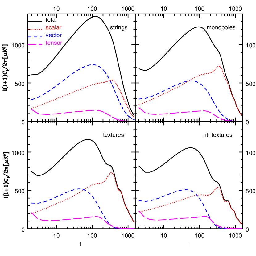
FIG. 1.: The contributions to the total anisotropy power spectrum from scalar, vector and tensor components, in the theories of global strings, monopoles, texture and nontopological texture (taken from ref. [1]).

II Causality and Analyticity

As discussed in [5], all perturbation power spectra are determined by the unequal time correlator (UETC) of the defect source stress energy tensor $\Theta_{\mu\nu}$:

$$\langle\Theta_{\mu\nu}({\bf k},\tau)\Theta_{\rho\lambda}(-{\bf k},\tau^{\prime})\rangle\equiv{\cal C}_{\mu\nu,\rho\lambda}(k,\tau,\tau^{\prime})$$ (1)

where $\tau$, $\tau^{\prime}$ denote conformal time, and $k$ comoving wavenumber. Note that (1) is real because complex conjugation is equivalent to the replacement ${\bf k}\rightarrow-{\bf k}$. The correlators are invariant under this replacement because the statistical ensemble is rotation invariant.

Causality means that the real space correlators of the fluctuating part of $\Theta_{\mu\nu}$ must be zero for $r>\tau+\tau^{\prime}$ [4]. Scaling dictates that in the pure matter or radiation eras ${\cal C}_{\mu\nu,\rho\lambda}\propto\phi_{0}^{4}/(\tau\tau^{\prime})^{1\over 2}c_{\mu\nu,\rho\lambda}(k\tau,k\tau^{\prime})$, where $\phi_{0}$ is the symmetry breaking scale and $c$ is a dimensionless scaling function. Finally, $\Theta_{\mu\nu}$ must obey the equations for stress energy conservation with respect to the background metric (see next Section). These provide two linear constraints on the four scalar components of the source. Any pair determines the other two up to possible integration constants. In the matter era the pair $\Theta$ and $\Theta^{S}$ [5] provides a convenient choice, allowing an analytical integral solution to the linearised Einstein equations. But for work including the matter-radiation transition [1] the pair $\Theta_{00}$ and $\Theta^{S}$ is better, because it results in the correct redshifting away of all components of the source stress energy inside the horizon. In this paper we shall use both pairs - $\Theta$ and $\Theta^{S}$ in our analytical discussion of an ‘incoherent’ model, and $\Theta_{00}$ and $\Theta^{S}$ for a numericaly solved ‘coherent’ model. In the former case, we shall constrain $\Theta$ and $\Theta^{S}$ so that on subhorizon scales the source is negligible (see Section IV).

The unequal time correlator in $k$ space is the Fourier transform of the real space correlator: $\langle\Theta_{ij}({\bf k},\tau)\Theta_{kl}(-{\bf k},\tau^{\prime})\rangle=\int d^{3}{\bf r}e^{-i{\bf k.r}}\langle\Theta_{ij}(r,\tau)\Theta_{kl}(0,\tau^{\prime})\rangle$. The integral is finite because the real space correlator has compact support, and it follows that the unequal time correlators are analytic in ${\bf k}$ for all finite $k$. They may thus be expanded as Taylor series in the Cartesian components $k_{i}$ about $k_{i}=0$. As $k_{i}$ tends to zero, isotropy and symmetry impose

$${\rm Lim}\quad{\bf k}\rightarrow 0\quad\langle\Theta_{ij}({\bf k},\tau)\Theta_{kl}(-{\bf k},\tau^{\prime})\rangle=A\delta_{ij}\delta_{kl}+B(\delta_{ik}\delta_{jl}+\delta_{il}\delta_{jk})$$ (2)

with $A$ and $B$ independent of ${\bf k}$.

The trace scalar, anisotropic scalar, vector and tensor components of a tensor $T_{ij}$ are given by

$$T_{ij}({\bf k}) = {1\over 3}\delta_{ij}T+(\hat{k}_{i}\hat{k}_{j}-{1\over 3}\delta_{ij})T^{S}+(\hat{k}_{i}T^{V}_{j}+\hat{k}_{j}T^{V}_{i})+T^{T}_{ij}$$ (3)

$$T_{i}^{V}k_{i} = k_{i}T^{T}_{ij}=T^{T}_{ij}k_{j}=T^{T}_{jj}=0,$$ (4)

where $\hat{k}_{i}\equiv k_{i}/k$. Expressing the trace $T$, $T^{S}$, $T_{i}^{V}$ and $T_{ij}^{T}$ in terms of $T_{ij}$ (see e.g. [5]) one finds that the only nonzero correlators consistent with statistical isotropy and homogeneity are $\langle TT\rangle$, $\langle TT^{S}\rangle$, $\langle T^{S}T^{S}\rangle$, $\langle T^{V}_{i}T^{V}_{j}\rangle$ and $\langle T^{T}_{ij}T^{T}_{kl}\rangle$. From (2) one can compute the small $k$ power spectra of the anisotropic scalar, vector and tensor stresses. One finds they are in the ratios

$$\langle|\Theta^{S}|^{2}\rangle:\langle|\Theta^{V}_{i}|^{2}\rangle:\langle|\Theta^{T}_{ij}|^{2}\rangle=3:2:4$$ (5)

where all indices are summed. Thus in a causal theory anisotropic scalar, vector and tensor stresses have white noise components at small $k$ with related amplitudes. A similar argument shows that the correlator $\langle\Theta_{00}\Theta_{ij}\rangle\sim{\rm C}\delta_{ij}$ at small $k$, implying that $\langle\Theta_{00}\Theta^{S}\rangle$ vanishes like $k^{2}$ at small $k$. Likewise $\langle\Theta\Theta^{S}\rangle$ vanishes like $k^{2}$ at small $k$. So for either of the two choices discussed above, the two scalar source components are uncorrelated outside the horizon.

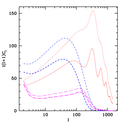
FIG. 2.: The importance of the long wavelength modes in the anisotropy power spectra from cosmic textures. The power spectra due to scalar (dotted), vector (dashed) and tensor (long-dashed) components of the sources are compared to those where the source stress energy components $\Theta_{00}$ and $\Theta^{S}$ as well as the vector and tensor stresses are set zero for all $k\tau>5$. The upper curves show the full spectra, the lower ones the results where the cutoff is imposed.

III Superhorizon Modes

In the cosmic defect theories, perturbations are predominantly produced on the horizon scale. Studies show that the unequal time correlators take the predicted white noise form for $k\tau<5$ or so, and decline strongly at larger $k\tau$. To the extent that the horizon scale modes reflect the causality constraints discussed above, the latter translate into definite relations between the scalar, vector and tensor perturbation power spectra. In Figures 2 and 3 we show the CMB anisotropy power spectra calculated in the cosmic global string and texture theories respectively, with and without a cutoff where we switch off the source stress tensor for $k\tau>5$. The Figures show that in the texture theory the effect of suppressing the source for $k\tau>5$ is relatively minor. For strings, there is a larger effect, but even here the ratios of scalar to vector to tensor anisotropies are not much affected. We conclude that the contributions from $k\tau<5$, which we shall term superhorizon modes, are certainly important in both theories and give at the least a rough measure of the importance of the scalar, vector and tensor contributions to the large angle anisotropies.

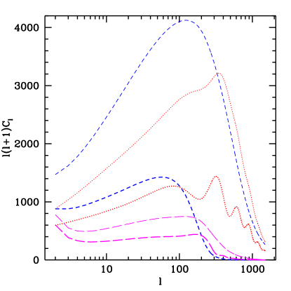
FIG. 3.: As in Figure 2 but for global strings.

IV Integral Constraints

The fact that a cutoff on subhorizon scales does not greatly affect the large angle $C_{l}$ spectrum has important implications. It means that the short distance structure of the individual defects is not important in determining the qualitative character of the large angle anisotropies, such as the relative scalar/vector/tensor contributions.

Consider the effect of modelling the sources using a ‘smoothed’ $\Theta_{00}$ tensor, one where we impose a cutoff at $k\tau\sim 5$. We feed in the smoothed $\Theta_{00}$ and $\Theta^{S}$ into the stress energy conervation equations:

$$\dot{\Theta}_{00}+\frac{\dot{a}}{a}(\Theta_{00}+\Theta)=\Pi;\qquad\dot{\Pi}+2\frac{\dot{a}}{a}\Pi=-\frac{k^{2}}{3}(\Theta+2\Theta^{S}).$$ (6)

where $\Pi=\partial_{i}\Theta_{0i}$ and $\Theta$ and $\Theta^{S}$ are defined in the previous Section. It is straightforward to see that the solutions for $\Pi$ and $\Theta$ are well defined.

In this scheme, we deduce important relations between $\Theta$ and $\Theta^{S}$. Equations (6) are easily integrated to obtain $\Theta_{00}$ in terms of $\Theta$ and $\Theta^{S}$: exchanging the order of the double integral we get

$$\Theta_{00}=\tau^{-2}\bigl{[}\int_{0}^{\tau}d\tau^{\prime}2\tau^{\prime}\Theta+{1\over 3}k^{2}\tau^{\prime 4}({1\over\tau^{\prime}}-{1\over\tau})(\Theta+2\Theta^{S})(\tau^{\prime})\bigr{]},$$ (7)

where we used $a(\tau)\propto\tau^{2}$ in the matter era. But as argued, the smoothed $\Theta_{00}$ is identically zero inside the horizon. It follows that both the $\tau^{-2}$ and $\tau^{-3}$ coefficients integrate to zero. The former gives

$$\int_{0}^{\infty}d\tau^{\prime}\bigl{[}2\tau^{\prime}\Theta+{1\over 3}k^{2}\tau^{\prime 3}(\Theta+2\Theta^{S})(k,\tau^{\prime})\bigr{]}=0,$$ (8)

and the latter gives

$$\int_{0}^{\infty}d\tau^{\prime}\tau^{\prime 4}(\Theta+2\Theta^{S})(k,\tau^{\prime})=0.$$ (9)

This imposes a negative correlation between $\Theta$ and $\Theta^{S}$, and guarantees that $\Pi$ vanishes faster than $a^{-2}$ inside the horizon. The constraints (8) and (9) will turn out to be remarkably powerful when building models for the superhorizon components of $\Theta$ and $\Theta^{S}$.

V Perturbations in the Matter Era

We wish to compute the large angular scale anisotropies produced in the matter era. For this purpose we use the following integral solution to the linearised Einstein equations in a matter dominated universe [5]:

$${\delta T\over T}({\bf n})|_{SW} = -{1\over 2}\int_{i}^{f}d\tau h_{ij,0}(\tau,{\bf n}(\tau_{0}-\tau))n^{i}n^{j};\qquad h_{ij,0}=h_{ij,0}^{\rm scalar}+h_{ij,0}^{\rm vector}+h_{ij,0}^{\rm tensor}$$ (10)

$$h_{ij,0}^{\rm scalar} = -16\pi G\sum_{\bf k}e^{i{\bf k}.{\bf x}}\int_{0}^{\tau}d\tau^{\prime}\bigl{[}{1\over 3}\delta_{ij}({\tau^{\prime}\over\tau})^{6}(\Theta+2\Theta^{S})(\tau^{\prime},{\bf k})-\hat{k}^{i}\hat{k}^{j}({\tau^{\prime}\over\tau})^{4}\Theta^{S}(\tau^{\prime},{\bf k})\bigr{]}$$ (11)

$$h_{ij,0}^{\rm vector} = \sum_{\bf k}e^{i{\bf k}.{\bf x}}(h_{i,0}^{V}\hat{k}_{j}+h_{j,0}^{V}\hat{k}_{i})\qquad h_{i,0}^{V}=16\pi G\int_{0}^{\tau}d\tau^{\prime}({\tau^{\prime}\over\tau})^{4}\Theta_{i}^{V}(\eta^{\prime})$$ (12)

$$h_{ij,0}^{\rm tensor}(\tau,{\bf x}) = 16\pi G\int_{0}^{\tau}d\tau^{\prime}k^{3}\tau^{\prime 4}\bigl{[}G_{1}(\tau^{\prime})\dot{G}_{2}(\tau)-G_{2}(\tau^{\prime})\dot{G}_{1}(\tau)\bigr{]}\Theta_{ij}^{T}(\tau^{\prime}{\bf x})$$ (13)

$$G_{1}(\tau) = {{\rm cos}(k\tau)\over(k\tau)^{2}}-{{\rm sin}(k\tau)\over(k\tau)^{3}};\quad G_{2}(\tau)={{\rm cos}(k\tau)\over(k\tau)^{3}}+{{\rm sin}(k\tau)\over(k\tau)^{2}};$$ (14)

where $G_{1}$ and $G_{2}$ are the two homogenous solutions to the tensor (gravity wave) equation.

The model we shall consider is one in which the components of $\Theta_{ij}$ have the following unequal time autocorrelators:

$$(16\pi G)^{2}\langle\Theta({\bf k},\tau)\Theta(-{\bf k},\tau^{\prime})\rangle = \theta(\epsilon-k\tau)\delta(\tau-\tau^{\prime}){\cal A}$$ (15)

$$(16\pi G)^{2}\langle\Theta^{S,V,T}({\bf k},\tau)\Theta(-{\bf k},\tau^{\prime})^{S,V,T}\rangle = \theta(\epsilon-k\tau)\delta(\tau-\tau^{\prime}){\cal A}^{S,V,T}$$ (16)

where $\theta$ is the Heaviside function, and we define $\langle\Theta^{T}(\tau)\Theta^{T}(\tau^{\prime})\rangle\equiv{1\over 4}\langle\Theta_{ij}^{T}(\tau)\Theta_{ij}^{T}(\tau^{\prime})\rangle$, and $\langle\Theta^{V}(\tau)\Theta^{V}(\tau^{\prime})\rangle\equiv{1\over 2}\langle\Theta_{i}^{V}(\tau)\Theta_{i}^{V}(\tau^{\prime})\rangle$, with all indices summed.

The sources are nonzero only on ‘superhorizon’ scales ($k\tau<\epsilon$) and they are uncorrelated except at equal times. This latter property means that the model is ‘totally incoherent’, in the terminology of ref. [3]. These correlators are not strictly causal - in real space they take the form $r^{-3}\bigl{[}{\rm sin}x-x{\rm cos}x]$ where $x=\epsilon r/\tau$ - but they are small and oscillatory beyond $r\sim\tau$ for $\epsilon=5$. So the violations of causality are small. Rotational invariance forbids any cross-correlation between scalar, vector or tensor modes. There is however one more allowed cross correlator, namely that between the isotropic and anisotropic stresses. The argument given in Section III implies that $\langle\Theta\Theta^{S}\rangle$ vanishes as $k^{2}$ for small $k$, but it cannot be zero because of the constraint (9). We choose to model it as

$$(16\pi G)^{2}\langle\Theta({\bf k},\tau)\Theta^{S}(-{\bf k},\tau^{\prime})\rangle=\theta(\epsilon-k\tau)\delta(\tau-\tau^{\prime})\bigl{(}{k\tau\over\epsilon}\bigr{)}^{2}{\cal A}^{\Theta S}$$ (17)

If we now compute the equal time correlator of the the constraint (9), we determine

$${\cal A}^{\Theta S}=-{11\over 36}({\cal A}+4{\cal A}^{S}).$$ (18)

Similarly we compute the equal time correlator of (8) and obtain

$$({4\over 3}+{4\over 15}\epsilon^{2}+{1\over 63}\epsilon^{4}){\cal A}+({8\over 21}\epsilon^{2}+{4\over 81}\epsilon^{4}){\cal A}^{\Theta S}+{4\over 63}\epsilon^{4}{\cal A}^{S}=0.$$ (19)

These equations yield ${\cal A}^{\Theta S}=-2.47{\cal A}^{S}$ and ${\cal A}=4.07{\cal A}^{S}$ for $\epsilon=5$. At $k\tau=5$, there is a mild inconsistency with the bound ${\cal A}^{\Theta S}<\sqrt{{\cal A}{\cal A}^{S}}$, so we shall adopt ${\cal A}^{\Theta S}=-2{\cal A}^{S}$ and ${\cal A}=4{\cal A}^{S}$.

VI The Delta Function Approximation

The procedure is simple in principle: the correlators (16) translate into correlators of the metric perturbations and thus into correlators of the temperature perturbations, equivalent to the anisotropy power spectrum $C_{l}$. But in order to compute the relevant integrals analytically, we shall make two approximations. The first is that we shall replace metric perturbation unequal time correlators under $\tau$ integrals using the following formula:

$$\langle\dot{A}(\tau)\dot{B}(\tau^{\prime})\rangle \rightarrow \delta(\tau-\tau^{\prime}){d\over d\tau}\langle A(\tau)B(\tau)\rangle$$ (20)

The weighting function is chosen so that the integrals $\int_{0}^{\tau_{f}}d\tau\int_{0}^{\tau_{f}}d\tau^{\prime}$ of both sides are guaranteed to be equal for all $\tau_{f}$. The formula is also invariant under changing variables from $\tau$ to any other function $f(\tau)$. The second approximation is to use the fact that the Greens functions in (14) fall off strongly with $\tau$. This means that the metric perturbations fall off rapidly beyond $k\tau=\epsilon$, which justifies us simply setting them zero beyond that point.

VII CMB Anisotropies

In the usual way we expand the microwave sky temperature in spherical harmonics $\delta T/T=\sum a_{lm}Y_{lm}(\theta,\phi)$, and compute $C_{l}=\langle|a_{lm}|^{2}\rangle$. The formulae for the contribution to the integrated Sachs Wolfe effect from trace scalar and anisotropic scalar contributions are [7]:

$$C_{l}^{scalar}={1\over 2\pi}\int_{0}^{\infty}k^{2}dk\langle\bigl{[}\int_{0}^{\tau_{0}}d\tau\bigl{(}{1\over 3}\dot{h}_{1}(\tau)+\dot{h}_{2}(\tau){d^{2}\qquad\over d(k\Delta\tau)^{2}}\bigr{)}j_{l}(k\Delta\tau)\bigr{]}^{2}\rangle$$ (21)

where $\Delta\tau=\tau_{0}-\tau$, $\tau_{0}$ is the conformal time today and as above, $\langle\rangle$ denotes ensemble averaging. The scalar metric perturbation components are given from (14):

$$\dot{h}_{1} = -16\pi G\int d\tau^{\prime}(\tau^{\prime}/\tau)^{6}(\Theta+2\Theta^{S})(\tau^{\prime})$$ (22)

$$\dot{h}_{2} = -16\pi G\int d\tau^{\prime}(\tau^{\prime}/\tau)^{4}\Theta^{S}(\tau^{\prime})$$ (23)

with ${\bf k}$ dependence implicit.

The vector and tensor contributions to $C_{l}$ are [7]

$$C_{l}^{V} = {2\over\pi}\int_{0}^{\infty}k^{2}dkl(l+1)\langle\bigl{[}\int_{0}^{\tau_{0}}d\tau\dot{h}^{V}(\tau){d\qquad\over d(k\Delta\tau)}\bigl{(}j_{l}(k\Delta\tau)/k\Delta\tau\bigr{)}\bigr{]}^{2}\rangle$$ (24)

$$C_{l}^{T} = {1\over 2\pi}\int_{0}^{\infty}k^{2}dk{(l+2)!\over(l-2)!}\langle\bigl{[}\int_{0}^{\tau_{0}}{d\tau\over k^{2}\Delta\tau^{2}}\dot{h}^{T}(\tau)j_{l}(k\Delta\tau)\bigr{]}^{2}\rangle$$ (25)

where $\langle\dot{h}^{T}(\tau)\dot{h}^{T}(\tau^{\prime})\rangle\equiv{1\over 4}\langle\dot{h}_{ij}^{T}(\tau)\dot{h}_{ij}^{T}(\tau^{\prime})\rangle$, and $\langle\dot{h}^{V}(\tau)\dot{h}^{V}(\tau^{\prime})\rangle\equiv{1\over 2}\langle\dot{h}_{i}^{V}(\tau)\dot{h}_{i}^{V}(\tau^{\prime})\rangle$, with all indices summed.

We now compute the relevant metric perturbation correlators: from (16), (18) and (23), using ${\cal A}^{\Theta S}=-2{\cal A}^{S}$ and ${\cal A}=4{\cal A}^{S}$ as discussed above, we obtain

$$\langle h_{1}(\tau)^{2}\rangle \approx {1\over 40}\tau^{3}{\cal A}^{S}$$ (26)

$$\langle h_{2}(\tau)^{2}\rangle = {1\over 81}\tau^{3}{\cal A}^{S}$$ (27)

$$\langle h_{1}(\tau)h_{2}(\tau)\rangle \approx {1\over 217}\tau^{3}{\cal A}^{S}$$ (28)

$$\langle h^{V}(\tau)^{2}\rangle = {1\over 81}\tau^{3}{\cal A}^{V}$$ (29)

$$\langle h^{T}(\tau)^{2}\rangle = \int_{0}^{\tau}d\tau^{\prime}G(\tau,\tau^{\prime})^{2}{\cal A}^{T}$$ (30)

$$G(\tau,\tau^{\prime}) = k^{3}\tau^{\prime 4}\bigl{[}G_{1}(\tau^{\prime})G_{2}(\tau)-G_{2}(\tau^{\prime})G_{1}(\tau)\bigr{]}$$ (31)

where we have evaluated the scalar correlators at $k\tau=5$, and the tensor modes $G_{1}$ and $G_{2}$ are given in equation (14). The tensor integral is straightforwardly performed, yielding

$$\langle h^{T}(\tau)^{2}\rangle = {{\cal A}^{T}\over 60k^{3}z^{6}}\bigl{(}{105\over 2}(1-z^{2}){\rm sin}(2z)-105z{\rm cos}(2z)+6z^{7}-14z^{5}-35z^{3}\bigr{)}$$ (32)

where $z=k\tau$. This function is $\sim{\cal A}^{T}\tau^{3}/81$ at small $k\tau$, identical to the vector expression. But for larger $k\tau$ it is suppressed, with the suppression factor being $\approx 0.29$ at $k\tau=5$. The suppression is due to the oscillatory nature of the tensor compared to the vector response.

We now compute the integrals in (25), starting with the tensor contribution $C_{l}^{T}$. The delta function allows one of the $\tau$ integrals to be performed. Then we change variables from $k$ to $x=k\Delta\tau$. The Heaviside function gives the upper limit $x<\epsilon(\tau_{0}/\tau-1)$, or $\tau<\tau_{0}/(1+x/\epsilon)$. Exchanging orders of the integrals we find

$$C_{l}^{T} = {1\over 2\pi}{(l+2)!\over(l-2)!}\int_{0}^{\infty}{dx\over x^{2}}j_{l}^{2}(x)\int_{0}^{\tau_{0}/(1+x/\epsilon)}{d\tau\over(\tau_{0}-\tau)^{3}}{d\over d\tau}\langle h^{T}(\tau)^{2}\rangle$$ (33)

For large $l$ the integral is dominated by large $x$, since $j_{l}(x)\sim x^{l}$ at small $x$. But at large $x$, $\tau<<\tau_{0}$ and the $\tau$ integral is trivial. Thus one finds at large $l$

$$C_{l}^{T}\sim.29{\epsilon^{3}\over 81}{\cal A}^{T}{l^{4}\over 2\pi}\int_{0}^{\infty}{dx\over x^{5}}j_{l}^{2}(x)\sim 0.29{\epsilon^{3}\over\pi}{\cal A}^{T}{2\over 1215l^{2}}+o(l^{-3}).$$ (34)

where we have used

$$\int dxj_{l}^{2}(x)x^{n}={\pi\over 2^{2-n}}{\Gamma(1-n)\Gamma(l+{1\over 2}+{n\over 2})\over\Gamma(1-{n\over 2})^{2}\Gamma(l+{3\over 2}-{n\over 2})}.$$ (35)

We have computed the integral for the tensor contribution (33) at low $l$ using Mathematica, to check that the model reproduces the shape of $l(l+1)C_{l}$ seen in the plots of Figure 1. Figure 4 confirms that this is indeed the case.

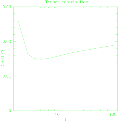
FIG. 4.: Tensor anisotropy power spectrum as computed in the analytical model presented here.

The vector integral is performed similarly, to obtain

$$C_{l}^{V}={1\over 27}{\cal A}^{V}{2l(l+1)\over\pi}\int_{0}^{\infty}dxx^{2}[(j_{l}(x)/x)^{\prime}]^{2}\bigl{[}{\epsilon^{2}\over 2x^{2}}-{\epsilon\over x}+{\rm ln}(1+\epsilon/x)\bigr{]}.$$ (36)

where prime denotes differentiation with respect to $x$. Approximating the square bracket with its leading large $x$ behaviour, integrating by parts and using Bessel’s equation for $j_{l}(x)$, we obtain at large $l$

$$C_{l}^{V}\sim{\cal A}^{V}{2\epsilon^{3}\over 1215\pi l^{2}}+o(l^{-3}).$$ (37)

The scalar contribution is evaluated using (20) and (23), again making the large $x$ approximation, giving

$$C_{l}^{scalar}={\cal A}^{S}{1\over 2\pi}\int_{0}^{\infty}x^{2}dx({1\over 120}j_{l}^{2}+{1\over 81}j_{l}^{\prime\prime 2}+{4\over 217}j_{l}j_{l}^{\prime\prime})(x){\epsilon^{3}\over 2x^{3}}.$$ (38)

After integrations by parts and using Bessel’s equations we get

$$C_{l}^{scalar}\approx{1\over 1248}{\cal A}^{S}{\epsilon^{3}\over\pi l^{2}}+o(l^{-3}).$$ (39)

Now the amplitudes ${\cal A}^{S}$, ${\cal A}^{V}$ and ${\cal A}^{T}$ are related via (5) in the ratio 3: 1: 1. Thus in the various approximations we have made, the ratio of the scalar to vector to tensor contributions to the large angle anisotropies are

$$C_{l}^{scalar}:\quad C_{l}^{V}:\quad C_{l}^{T}=1.46:\quad 1:\quad 0.29$$ (40)

which is our main result. The calculation demonstrates the relative importance of the vector and tensor modes, consistent with the numerical results shown in Figure 1. Given the crude nature of the model used, the agreement is actually surprisingly good. The weakest point in the model is that it involves a free parameter $\epsilon$, and the $C_{l}$’s obtained are proportional to $\epsilon^{3}$. It seems plausible that $\epsilon$ should be the same for the scalar, vector and tensor stresses, but we have not found any argument as to why this should necessarily be true.

Let us summarise the approximations and assumptions implicit in (40):

$\bullet$ We assumed that superhorizon modes with $k\tau<5$ dominate.

$\bullet$ We modelled the unequal time correlators as delta functions with a horizon scale cutoff.

$\bullet$ We made the approximation of pure matter domination for the background spacetime. In this approximation the $C_{l}$ spectra obtained are scale invariant at large $l$.

$\bullet$ We replaced certain functions with amplitudes times delta functions in order to perform the relevant integrals.

With all of these caveats, we feel that the model provides useful insight into the relative importance of scalar, vector and tensor contributions to the large angle anisotropies. The model explains why vector perturbations dominate over tensors, and why the combined vector and tensor contribution is comparable to that from scalars.

VIII Numerical Solution of a Coherent Model

As a further model we have considered the case of a completely coherent source in which the unequal time correlators of $\Theta_{00}$, $\Theta^{S}$, $\Theta^{T}$, and $\Theta^{V}$ are all proportional to the product of Heaviside functions, for example setting

$$\langle\Theta_{00}({\bf k},\tau)\Theta_{00}(-{\bf k},\tau^{\prime})\rangle=(\tau\tau^{\prime})^{-{1\over 2}}\Theta(\epsilon-k\tau)\Theta(\epsilon-k\tau^{\prime}).$$ (41)

Note that we need to model the white noise $\Theta^{S}$ contribution, but as mentioned above, the cross correlator must vanish at small $k$. So in this model we will assume that $<\Theta_{00}\Theta^{S}>$ is identically zero, and therefore solve for the $\Theta_{00}$ and $\Theta^{S}$ contributions separately. Note that with this choice of variables, the constraints (8) and (9) are automatically satisfied.

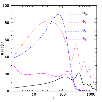
FIG. 5.: Angular power spectrum of anisotropies generated by a simple coherent model of scaling sources, correctly incorporating the superhorizon constraints on the relative importance of the anisotropic stress $\Theta^{S}$, vector $\Theta^{V}$ and tensor $\Theta^{T}$ perturbations to the source stress tensor.

We have used this model in the full Boltzmann code developed in [1] as usual with $\epsilon=5$. The results are shown in Figure 5. The anisotropic scalar, vector and tensor $C_{l}$’s have been scaled so that the stress tensor white noise superhorizon amplitudes are in the correct ratios (5). $C_{l}^{00}$ has been scaled with $C_{l}^{S}$. It is a remarkably small contribution. This may be understood by solving the equations for stress energy conservation for $\Theta$, whence one finds that $\Theta$ is actually very small in the coherent model at horizon crossing $k\tau\sim 5$, so that from (14) its contribution to the anisotropy is small.

The coherent model provides a useful comparison to the previous incoherent model. The broad agreement between the two models suggests that our main result (40) is actually insensitive to the detailed nature of the source. An advantage of the coherent model is that we can more easily incorporate the matter-radiation transition, giving rise to departures from scale invariance in the $C_{l}$ spectrum qualitatively similar in character to those observed in the realistic source calculations. And as seen in Figure 5 the model gives a reasonable impression of the main features of the realistic calculations in Figure 1, at least on large angular scales.

IX Conclusions

In this paper we have developed a set of physically reasonable models for the perturbations generated on superhorizon scales by causal sources. We gave some rigorous and some approximate arguments that the large angular scale anisotropies due to the scalar and vector plus tensor modes are in general similar in magnitude. If the vector and tensor contributions to the large angle anisotropies are large, the scalar normalisation is lower and the Doppler peaks due to scalar perturbations are small compared to the large angle Sachs-Wolfe plateau.

Let us close by mentioning some loopholes in the above arguments, which make it possible to circumvent the conclusion that causal sources are unlikely to have large Doppler peaks.

$\bullet$ If subhorizon modes with $k\tau>5$ dominate the anisotropies then our arguments do not apply. Sources in this category have been explored by Durrer and Sakellariadou [8].

$\bullet$ If the shape of the unequal time correlators, parametrised in our models by $\epsilon$ is different for the scalar, vector and tensor components, then the $C_{l}$ contributions could be strongly affected, since $C_{l}\propto\epsilon^{3}$. One could imagine a model where $\epsilon$ for scalars was larger than for vectors and tensors, but even here one would probably not find sharp Doppler peaks, since increasing $\epsilon$ is likely to increase the incoherence of the source and thus smoothe out the Doppler peaks (this is apparent in Figures 2 and 3).

$\bullet$ One could consider sources like those in [4] in which the anisotropic stresses are by construction zero outside the horizon. In such a model the superhorizon constraint (5) is satisfied with all terms being zero. In the model of [4] this is true because the real space stress energy master functions were taken to be spherically symmetric, clearly a special case.

$\bullet$ We have assumed perfect scaling of the sources, and matter domination. There is some violation of scaling due to the matter-radiation transition, but this is a small effect on large angular scales. Stronger departures from scaling would result from a non-minimal-coupling mass term $R\theta^{2}$ for the Goldstone bosons. We are currently exploring this possibility.

X Acknowledgements

We thank A. Albrecht, R. Battye and J. Robinson for helpful discussions.

REFERENCES

• [1] U. Pen, U. Seljak and N. Turok, preprint DAMTP-97-36, astro-ph/9704165; preprint DAMTP-97-35, astro-ph/9704231.
• [2] B. Allen, R. R. Caldwell, S. Dodelson, L. Knox, E. P. S. Shellard, A. Stebbins, preprint astro-ph/9704160 (1997).
• [3] A. Albrecht, D. Coulson, P. Ferreira and J. Magueijo, Phys. Rev. Lett. 76, 1413 (1996).
• [4] N. Turok, Phys. Rev. D54, 3686 (1996), Phys. Rev. Lett., 77, 4138 (1996).
• [5] U. Pen, D. Spergel and N. Turok, Phys. Rev. D48 , 692 (1994).
• [6] U. Pen, U. Seljak and N. Turok, 1997, in preparation.
• [7] R. Crittenden and N. Turok, Phys. Rev. Lett. 75, 2642 (1995).
• [8] R. Durrer and M. Sakellariadou, U. Geneva preprint 1997, astro-ph/9702028.