Cosmic Microwave Background Anisotropies from Scaling Seeds:
Fit to Observational Data

Abstract

We compute cosmic microwave background angular power spectra for scaling seed models of structure formation. A generic parameterization of the energy momentum tensor of the seeds is employed. We concentrate on two regions of parameter space inspired by global topological defects: ${\cal O}(4)$ texture models and the large-$N$ limit of ${\cal O}(N)$ models. We use $\chi^{2}$ fitting to compare these models to recent flat-band power measurements of the cosmic microwave background. Only scalar perturbations are considered.

Inflation and topological defects are two families of models to explain the origin of large scale structure in the universe. In models with topological defects or other types of seeds, fluctuations are generated continuously and evolve according to inhomogeneous linear perturbation equations. Seeds are any non-uniformly distributed form of energy, which contributes only a small fraction to the total energy density of the universe and which interacts with the cosmic fluid only gravitationally. We are particularly interested in global topological defects playing the role of seeds.

Cosmic microwave background (CMB) anisotropies provide a link between theoretical predictions and observational data, which may allow us to distinguish between inflationary perturbations and defects, by purely linear analysis. On large angular scales, both families of models predict an approximately scale-invariant Harrison-Zel’dovich spectrum [1, 2]. For inflationary models this can be seen analytically. Scale-invariance for defects was discovered numerically [3, 4, 5]; simple analytical arguments are given in [6]. At small angular scales ($0^{\circ}\!\!.2\stackrel{{\scriptstyle<}}{{\sim}}\theta\stackrel{{\scriptstyle<}}{{\sim}}1^{\circ}$), the predictions of inflation and defects are different. CMB observations at these scales may soon be sensitive enough to distinguish the two families of models.

In a recent work [7], two of us investigated the general behavior of CMB anisotropies induced by seeds. Here, for simplicity, we restrict ourselves to scalar type perturbations. Thus, the models presented in this work are not close approximations to the ${\cal O}(4)$ texture model for which the Sachs-Wolfe (SW) plateau is dominated by vector and tensor modes [8, 9].

This restriction does not render our work uninteresting. There may very well be models with scaling seeds leading to small vector and tensor contributions, e.g., due to symmetry constraints (spherical symmetry) or in models with non-relativistic seeds. Here, we assume a completely phenomenological standpoint: we investigate whether models with purely scalar seeds can reproduce the data. In subsequent work we plan to study how severely vector and tensor contributions are restricted by the data. However, the models already excluded on the basis of our work, will not be resurrected once vector and tensor modes are included.

In our models, we characterize the energy momentum tensor of the source by four seed functions which we term $f_{\rho},~{}f_{p},~{}f_{v},$ and $f_{\pi}$, defined by (see [10, 11])

$$\Theta_{00} = M^{2}f_{\rho}$$ (1)

$$\Theta^{(s)}_{i0} = M^{2}f_{v,i}$$ (2)

$$\Theta^{(s)}_{ij} = M^{2}[\{f_{p}-(1/3)\Delta f_{\pi}\}\gamma_{ij}+f_{\pi|ij}]~{},$$ (3)

where $\Delta$ denotes the Laplacian and _| is the covariant derivative with respect to the metric $\gamma$ of three space. $M$ is a typical “mass”, or energy scale, of the seeds. The gravitational strength of the seeds is characterized by the dimensionless parameter $\epsilon=4\pi GM^{2}$. The superscript ^(s) indicates that only the scalar contribution to $\Theta_{i0}$ and $\Theta_{ij}$ is included here. Since seeds interact with other matter components only gravitationally, the seed functions satisfy the covariant conservation equations [10]

$$\dot{f}_{\rho}-\Delta f_{v}+(\dot{a}/a)(f_{\rho}+3f_{p}) = 0$$ (4)

$$\dot{f}_{v}+2(\dot{a}/a)f_{v}-f_{p}-(2/3)\Delta f_{\pi} = 0~{},$$ (5)

where $a$ is the scale factor and dot stands for derivative with respect to conformal time $t$.

We define “scaling seeds” to be seeds for which the power spectra $\langle|f_{\bullet}|^{2}\rangle(k,t)$ are, up to an overall power of $t$ determined by dimensional reasons, functions of $x=kt$ only. Thus, the power spectra of the functions $f_{\bullet}$ are of the form

$$\langle|f_{\rho}|^{2}\rangle = t^{-1}~{}F_{1}^{2}(x)$$ (6)

$$\langle|f_{p}|^{2}\rangle = t^{-1}~{}F_{2}^{2}(x)$$ (7)

$$\langle|f_{v}|^{2}\rangle = t~{}F_{3}^{2}(x)$$ (8)

$$\langle|f_{\pi}|^{2}\rangle = t^{3}~{}F_{4}^{2}(x)~{}.$$ (9)

Furthermore, we require that the seeds decay on sub-horizon scales. This behavior is found in simulations for the seed functions of global textures and is also supported by the large-$N$ limit of global ${\cal O}(N)$ models [12, 13]. Simple analytical arguments indicate that all types of models with scaling seed functions which decay fast enough inside the horizon lead to a Harrison-Zel’dovich spectrum[14].

Numerical simulations of global ${\cal O}(N)$ models show that on super-horizon scales ($x\ll 1$), $\Theta_{ij}$ and $\Theta_{00}$ have white noise spectra , whereas $|\Theta_{i0}|^{2}$ behaves like $k^{2}$. Furthermore, the power spectra of the functions $f_{\bullet}$ do not depend on the direction of k. Thus the $F_{i}$’s are even functions of $x=kt$. Consequently, $F_{1},F_{2},F_{3}\rightarrow$ const., while $F_{4}\propto 1/x^{2}$ for $x\rightarrow 0$. Since the energy momentum tensor of the seeds decays inside the horizon, $F_{i}\rightarrow 0$ for $x\rightarrow\infty$. In this work we approximate the random variables $f_{\bullet}$ by the square root of their power spectra. Motivated by numerical simulations and the considerations described above we model the functions $F_{1},F_{3}$ as

$$F_{1}={A_{1}\over 1+\alpha_{1}x^{n_{1}}}~{}~{}~{},~{}~{}~{}~{}~{}F_{3}={A_{3}\over 1+\alpha_{3}x^{n_{3}}}~{}.$$ (10)

$F_{2}$ and $F_{4}$ are then given by energy momentum conservation, Eqs. (4, 5).

The gravitational action of the seeds is determined by the induced Bardeen potentials, which are not only due to the seeds but also contain contributions from the matter and radiation fluids. Once the fluid perturbations and the Bardeen potentials are determined, one calculates CMB anisotropies by standard methods for each model parametrized by $(A_{1},\alpha_{1},n_{1},A_{3},\alpha_{3},n_{3})$. For details see Ref. [7].

In this letter we present the results of a parameter study and we fit to the observational data available. We compare the anisotropy power spectra obtained in our models with observations. The cosmological parameters used are $h=0.5,\Omega_{B}=0.0125h^{-2},\Omega=1$ and $\Lambda=0$. We are thus considering scaling seed models in the context of flat cold dark matter universes.

We investigate two types of models. In the first one we choose $n_{1}=2,~{}n_{3}=4$; a choice supported by numerical simulations of global textures [4]; we refer to this first type of scaling seed models as model A. In the second one we set $n_{1}=5/2$ and $n_{3}=7/2$; a result obtained analytically in the large-$N$ limit of ${\cal O}(N)$ models[12]. We call it model B.

We set the arbitrary normalization by fixing $A_{1}=1$ and we vary $A_{3}(=A_{3}/A_{1})$. To make the calculations feasible, we further reduce the remaining 3-dimensional parameter space $(A_{3},\alpha_{1},\alpha_{3})$ to 2-dimensions $(A_{3},\alpha_{1})$, by setting $\alpha_{3}=\alpha_{1}/2$. Thus, our fits are displayed as contour plots in the $\alpha_{1}-A_{3}$ plane (see Figs. 3 and 4). We have also investigated $\alpha_{3}=2\alpha_{1}$ and obtained qualitatively similar results.

The $A_{3}$ dependence is similar for both types of models. For $A_{3}\stackrel{{\scriptstyle<}}{{\sim}}0.06$, the relative amplitude of the acoustic peak, with respect to the SW plateau, decreases as $A_{3}$ decreases (see Figs. 1a and c).

There is a particular value of the constant $A_{3}$ for which the coefficient of the $1/x^{2}$ term in $F_{4}$ vanishes. For $x\ll 1$, one obtains from Eqs. (4,5) $F_{4}\approx A_{4}/x^{2}$ with $A_{4}=-(3/8)A_{1}(1+18A_{3}/A_{1})$ in the matter dominated era. If $A_{3}=(-1/18)A_{1}\equiv A_{crit}\sim-0.06$, we thus find $A_{4}=0$ [7]. This $1/x^{2}$ term dominates on super-horizon scales and (for big enough $\alpha_{i}$) determines the amplitude of the SW plateau. Its absence is thus expected to lead to a higher relative amplitude of the first acoustic peak, which is well visible in Figs. 1a and 1c.

FIG. 1.: Parameter dependence of the calculated power spectra. To illustrate the dependence on $A_{3}$, we choose values around $A_{crit}=-0.06$ (see text). The dotted line is a polynomial fit to the data and is the same in each panel as a reference.

FIG. 2.: Flat-band power measurements used in this analysis. The best-fit models of two scaling seed models are also shown: one most relevant to model A (Fig. 3) and the other for model B (Fig. 4).

In our exploration of parameter space we vary $-1.0\leq A_{3}\leq+1.0$ for model A and $-1.2\leq A_{3}\leq+0.5$ for model B. For $\alpha_{1}$ we choose the parameter range $0.01\leq\alpha_{1}\leq 2.0$ for model A and $0.001\leq\alpha_{1}\leq 0.141$ for model B. We normalize the power spectra at $\ell=10$ by fitting to the data.

We use $\chi^{2}$ fitting to compare our models to recent flat-band power measurements of the CMB. The method and a compilation of the data is described in detail in [15]. The most recent data and improvements to the $\chi^{2}$ method are described in [16, 17].

Fig. 2 plots the data used along with the best-fit power spectra for the two types of models described above. These best-fit models are indicated by the “X” in Figs. 3 and 4. Fig. 3 is a contour plot in the $\alpha_{1}-A_{3}$ plane for model A while Fig. 4 is the analogous one for model B.

There are 32 data points and 28 degrees of freedom (28 = 32 - 2 (fitted defect parameters) - 1 (normalization) - 1 (sliding Saskatoon absolute calibration)). Model A yields a $\chi^{2}$ minimum value $\chi_{\min}^{2}=21.2$, while model B yields $\chi_{\min}^{2}=27.1$. Thus the fits are good.

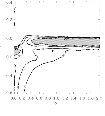
FIG. 3.: $\chi^{2}$ fit of model A to the CMB data. The “${\bf X}$” marks the $\chi^{2}_{min}$; the grey area is the $(\chi^{2}_{min}+1)$, $\sim 1\sigma$-likelihood region. Contours marked “68”, “95” and “99” refer to goodness-of-fit contours. For example, under the assumption that the errors on the flat-band power measurements are Gaussian, the probability of obtaining a $\chi^{2}$ value less than the value obtained on the “95” contour is $95\%$.

To interpret our $\chi^{2}$ fits, we first note the following: if perturbations decay fast enough, the height of the first acoustic peak is determined by $f_{\rho}+3f_{p}\sim A_{1}/4$, while the SW plateau is fixed by $A_{4}$. The $\chi^{2}$ is then not expected to be very sensitive to $\alpha$. This indeed is seen in model B for $\alpha_{1}\stackrel{{\scriptstyle>}}{{\sim}}0.03$ (Fig. 4 and also Fig. 1 b) and in model A for $\alpha_{1}\stackrel{{\scriptstyle>}}{{\sim}}0.4$ (Fig. 3.).

We also have investigated the dark matter power spectra for some of the parameter space of our models. For the best fitting models we obtain $\sigma_{8}\sim 0.6\pm 0.2$ which is in reasonable agreement with observations. Values of $(A_{3},\alpha_{1})$ which are excluded from the $C_{\ell}$ analysis, often lead to far too small values of $\sigma_{8}$. We found, however, that the bend in the power spectrum of our “best models” lies at somewhat smaller scales than in the analysis of APM and IRAS galaxies done by Peacock [18]. Since his analysis assumes Gaussian statistics, we are very reluctant to draw any strong conclusions from this comparison.

In the matter dominated era, numerical simulations of ${\cal O}(4)$-textures give $A_{1}\sim 4,\alpha_{1}\sim 0.012$ and $A_{3}\sim 0.37,\alpha_{3}\sim 0.05$ [13]. For this model, the scalar contribution to the SW plateau is $\sim 1.1\epsilon^{2}$ at $\ell\approx 10$ and the height of the first acoustic peak is about $\sim 5\epsilon^{2}$. On the other hand, full simulations, which include vector and tensor modes[4], lead to an amplitude of the SW contribution on the order of $\ell(\ell+1)C_{\ell}\sim 8^{+4}_{-2}\epsilon^{2}$. Therefore the vector and tensor parts contribute more than $\sim 80\%$ to the SW plateau, while they are not expected to influence the acoustic peaks. In the full texture models, the acoustic peaks are thus expected to be substantially too low to fit the data. This result was pioneered in [8] and has now been confirmed by full numerical simulations [9]. In Ref. [9] decoherence [19] has also been taken into account, which further reduces the acoustic peaks without influencing substantially the SW plateau.

The fact that we obtain a parameter range compatible with currently available observational data is clearly not in contradiction with the result of [8] and [9], namely that the acoustic peaks for the conventional ${\cal O}(4)$-texture model are very small or even completely absent.

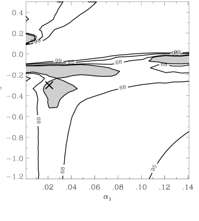
FIG. 4.: Same as previous figure except here we are fitting model B to the data.

Fig. 3 shows that small negative values of $A_{3}$ ($-0.1\leq A_{3}\leq 0$) are preferred. For $\alpha_{1}\stackrel{{\scriptstyle>}}{{\sim}}0.4$ the result does not depend strongly on $\alpha_{1}$. For smaller values of $\alpha_{1}$, ($\alpha_{1}\stackrel{{\scriptstyle<}}{{\sim}}0.2$) somewhat larger values of $|A_{3}|$ are preferred since the acoustic peaks are already enhanced due to the slower decay of the seed functions.

Fig. 4 is the model B analog of Fig. 3. Also here, a positive $A_{3}$ is excluded for $\alpha_{1}\stackrel{{\scriptstyle>}}{{\sim}}0.01$. A value of $A_{3}\sim-0.1$ is generically preferred. Note however, that the $\chi^{2}$ “landscape” within the parameter range explored in Figs. 3,4 is rather flat, and values within the “68” contour are reasonably compatible with current data.

In this letter, our aim was not to test whether a given model with topological defects can fit the data. We wanted to investigate, whether present observations of CMB anisotropies can already rule out a generic class of seed perturbations constrained just by energy momentum conservation and scaling arguments. Our analysis indicates that the answer to this question is no.

As a continuation of this work, we plan to include vector and tensor perturbations as well as decoherence in our models. We also want to study whether there are more severe restrictions on defect models than just energy momentum conservation and scaling; for example, to see whether the vector component always dominates the level of the SW plateau.

Acknowledgment      This work is partially supported by the Swiss NSF. M.S. acknowledges financial support from the Tomalla foundation. C.H.L acknowledges NSF/NATO post doctoral fellowship 9552722.

REFERENCES

- [1] H.R. Harrison, Phys. Rev. D1, 2726 (1970).
- [2] Y.B. Zel’dovich, Mon. Not. Roy. Ast. Soc. 160, 1 (1972).
- [3] U. Pen, D. Spergel and N. Turok, Phys. Rev. D49, 692 (1994).
- [4] R. Durrer and Z. Zhou, Phys. Rev. D53, 5394 (1996).
- [5] B. Allen at al., “Large Angular Scale CMB Anisotropy Induced by Cosmic Strings”, astro-ph/9609038 (1996).
- [6] R. Durrer, in Proceedings of the Workshop on Topological Defects in Cosmology, astro-ph/9703001 (1997).
- [7] R. Durrer and M. Sakellariadou, Phys. Rev. D56, 4480 (1997).
- [8] R. Durrer, A. Gangui and M. Sakellariadou, Phys. Rev. Lett. 76, 579 (1996).
- [9] U. Pen, U. Seljak and N. Turok “Power Spectra in Global Defect Theories of Cosmic Structure Formation”, astro-ph/97004165 (1997).
- [10] R. Durrer, Phys. Rev. D42, 2533 (1990).
- [11] R. Durrer, Fund. of Cosmic Physics 15, 209 (1994).
- [12] M. Kunz and R. Durrer, Phys. Rev. D55, 4516 (1997).
- [13] M. Kunz and R. Durrer, in preparation.
- [14] For models with decaying seeds, the Bardeen potentials are roughly constant inside the horizon. Therefore, the SW contribution is given by , where and prime stands for derivative w.r.t. . The lower boundary of the integrated term roughly cancels the ordinary SW contribution and the upper boundary leads, by simple dimensional reasons, to a Harrison-Zel’dovich spectrum.
- [15] C.H. Lineweaver, D. Barbosa, A. Blanchard and J. Bartlett, Astron. & Astrophys. 322, 365, astro-ph/9610133 (1997).
- [16] C.H. Lineweaver and D. Barbosa, Astron. & Astrophys. in press, astro-ph/9612146 (1997).
- [17] C.H. Lineweaver and D. Barbosa, Astrophys. J. 496, astro-ph/9706077 (1998).
- [18] J.A. Peacock Mont. Not. R. Astron. Soc. in press; astro-ph/9608151.
- [19] Decoherence is the decay of the correlation functions, , approximated here simply by . This is likely to influence the structure of the acoustic peaks.