Very rapid optical variability of PKS 2155-304

Abstract

We have performed an optical observation campaign on PKS 2155-304, whose aim was to determine the variability properties of this object on very short time scales in several photometric bands. We detected variability on time scales as short as 15 min.

The Fourier properties of the light curves have been investigated using structure function analysis. The power spectra are well described by a power-law with an index $-2.4$. It is compatible with the index found in the X-ray domain. The value of this index shows that the light curves cannot be generated by a sum of exponential pulses. Using historical data, we find that the longest time scale of variability in the optical domain lies between 10 and 40 days.

We find a strong correlation between flux and spectral index, which we interpret as the signature of an underlying constant component. As a result we do not find evidence of spectral variation for the active nucleus in the optical domain.

A lag has been found between the light curves in different optical bands. The short-wavelength light curves lead the long-wavelength ones. The amplitude of the lag is about 40 min for a factor 2 in wavelength.

Our results are compared with predictions from different models. None of them can explain naturally the set of results obtained with this campaign, but we bring out some clues for the origin of the variability.

Key words: BL Lacertae objects: individual: PKS 2155-304 – Galaxies: photometry

1 Introduction

Very soon after their discovery BL Lac objects were noted for their fast variability. As early as in ?, ? observed BL Lac with a time resolution of 15 s and recorded variations of 0.1 mag over a few hours. Since then, many BL Lac objects and active nuclei of other types are known to vary on time scales shorter than one day in the optical domain ?. These objects are usually classified as BL Lac objects and blazars, and have flat radio spectra. The very fast variability and the radio spectrum are often interpreted as the result of synchrotron emission from a Doppler-boosted jet.

PKS 2155-304 is the brightest BL Lac object in the optical domain, and is consequently very frequently observed. Variability on time scales of the order of one day has been observed by ?). In a 4-night campaign, they obtained a very smooth light curves, which is well eye-fitted by a unique sine function with a 3-day period. A drop of $\sim\!10$% has been detected in the ultraviolet in a few hours ?. ?) have studied EXOSAT observations of PKS 2155-304, and found that it was dominated by low-frequency variability, but detected variability on time scales of the order of 500 s. An important campaign has been performed in November 1991 with a very broad spectral coverage ????hereafter 1991-I, 1991-II, 1991-III, 1991-IV, respectively . The ultraviolet light curve showed some evidence of characteristic time scale of $\sim\!0.7$ days (1991-I). During this period, the optical and ultraviolet emissions were well correlated, without evidence of lag (1991-IV). The optical observations have been obtained from different ground-based telescopes (1991-III), which limited the accuracy of the observations. Moreover the sampling was not very dense. As a consequence, the optical variability pattern of PKS 2155-304 has not been fully explored.

In this paper we describe an optical campaign on PKS 2155-304 aiming at determining the properties of the variability of PKS 2155-304, with an emphasis on very short time scales. A limited spectral analysis has also been performed in five-colour photometry to study whether the hardness of the spectrum is related to the brightness of the source. We also investigate whether a lag can be detected between the different light curves. On the basis of our results, we make some inferences on the emission mechanism of the optical radiation in this object (and possibly in other BL Lac objects). A preliminary analysis of the data discussed here have been presented in ?).

2 Observations

2.1 The campaign

Table 1.: General information on the sampling. $n(\Delta t<10\mbox{ min})$ and $n(\Delta t<5\mbox{ min})$ are the number of consecutive observations separated by less than 10 min and 5 min respectively. $f_{\mathrm{Norm}}$ is the correction factor applied to the flux calibration (see Sect.2.3). The basic statistics of the observations are also given. $\sigma$ is the standard deviation of the light curves in physical units and $\tilde{\sigma}$ is the standard deviation in percentage of the mean flux. $\varepsilon_{\mathrm{SF}}$ is the uncertainty on the flux obtained from the structure functions (see Sect.4)

Filter	Exposure	Number of	$n(\Delta t<10\mbox{ min})$	$n(\Delta t<5\mbox{ min})$	$f_{\mathrm{Norm}}$	Mean Flux	$\sigma$	$\tilde{\sigma}$	$\varepsilon_{\mathrm{SF}}$
	time (s)	observations				mJy	mJy	%	mJy
UG	300	26	0	0	1.037	13.3	2.1	15.4	-
BG	180	110	49	0	0.958	15.5	2.3	14.7	0.12
VG	120	262	188	86	0.968	18.9	2.7	14.0	0.13
RG	60	224	144	70	1.052	21.8	2.7	12.2	0.09
IC	80	130	62	8	0.989	24.6	3.1	12.6	0.14

All observations were made with the 70-cm Geneva telescope at the European Southern Observatory in La Silla, Chile. The telescope is equipped with a CCD camera using a thick front-illuminated UV-coated GEC P8603 416x578 device ?. Besides the usual imager mode, the CCD camera can be operated as a multi-channel photometer. The filters that have been used in this campaign are the filters U, B and V from the Geneva photometric system (hereafter U_G, B_G and V_G to avoid confusion with Johnson’s filters; they are however comparable both in central wavelength and in width), a filter close to Gunn’s R filter (hereafter R_G) and a filter close to Cousins’ I filter (hereafter I_C).

The campaign started on July 26, 1995, and was supposed to last for 3 weeks. However, a bad-weather period prevented us to observe after Aug 9. This resulted in 15 consecutive nights of observation. We observed PKS 2155-304 as often as possible, with a rate strongly dependent on the filter. Filters V_G and R_G have been most frequently used. As the U_G observations were difficult to obtain, only one or two of them were performed each night to increase the spectral coverage. The exposure times have been estimated a priori to obtain a 1% accuracy on the flux (without taking into account the absolute flux calibration), which led us to make 2-min exposures in the V_G filter. The pointing and tracking limitations of the telescope reduced the operation period to about 5 hours per night, with a gap of about 45 min when PKS 2155-304 was too close to the zenith. Table 1 summarizes the observations performed during this campaign.

2.2 Data reduction

Only the relevant – user specified – areas of the CCD are read out, which enabled us to reduce significantly the delay between two observations. Images of repeated exposures are stored in a single structure and reprocessed off-line as follows. The raw flux of the object is obtained by integration within an aperture of $\sim\!20$ pixels (8 arc-seconds). The synthetic aperture is centered using a 2D profile fitting. The sky background is determined individually for each measurement using an average of the flux outside the integration zone. The (very rare) cosmic rays are detected and removed using the comparison with a fitted profile. The flat-field correction is made on the integrated flux rather than on the raw images (this is equivalent to the filtering of the flat fields). The data acquisition and image processing are carried out within the standard Geneva software called INTER ?. We perform differential photometry with a comparison star, which frees us from the problem of atmospheric extinction (the object and the comparison star are processed in exactly the same way). The parameters of the comparison star, which has been well measured in Geneva photometry, are: $V_{\mathrm{G}}=12.036$, $B_{\mathrm{G}}-V_{\mathrm{G}}=0.104$, $U_{\mathrm{G}}-V_{\mathrm{G}}=1.263$, $R_{\mathrm{G}}-V_{\mathrm{G}}=-0.367$ and $I_{\mathrm{C}}-V_{\mathrm{G}}=-0.752$. Its coordinates are $\alpha_{2000}=21\mbox{h\penalty 10000\kern 3.0pt}59\mbox{m\penalty 10000\kern 3.0pt}02.35\mbox{s}$, $\delta_{2000}=-30^{\circ}\penalty 10000\kern 3.0pt10^{\prime}\penalty 10000\kern 3.0pt46.5"$. In order to take advantage of the differential photometry we centred the field so that both the object and the comparison star lie in the same frame. Unfortunately, many observations had to be rejected, because one of the two sources had partially disappeared from the field of view during the observation, the angular distance between PKS 2155-304 and the comparison star being close to the size of the field of view.

Fig. 1.: Mean five-colour spectrum. The empty circles are the fluxes from the standard calibration, and the black squares are the fluxes corrected to obtain a power-law spectrum. The slope of the line is $-0.73$

2.3 Flux calibration

The absolute flux calibration of the Geneva photometric system ? was not intended to be used for active galactic nuclei. Spectrophotometric observations of PKS 2155-304 show that its spectrum is a featureless power-law (e.g. 1991-III). To obtain absolute flux calibration for PKS 2155-304, we estimate the most probable power-law spectrum, given by a least-squares linear regression, from the mean fluxes obtained with the standard calibration. The systematic deviations from the power-law spectrum are then corrected by the appropriate factor (at most 5%). Fig.1 shows the mean spectrum with the systematic deviations, and the correction factors for each filter are given in Table1.

2.4 Light curves

Fig. 2.: Light curves in the 5 filters in arbitrary units. The light curves are plotted in logarithm of the flux with an arbitrary normalization. The ticks on the $y$ axis indicate an increase in flux by a factor 1.5. The $x$ axis is not to scale

Fig. 3.: Examples of nights where very-short-term variability is clearly detected. The filter and the night number are given

Table1 gives the basic statistics of the data discussed here. Fig.2 shows the light curves in the five filters in logarithm of the flux with an arbitrary normalization. All the light curves look very similar. Fig.3 shows details of 4 nights in the V_G and R_G filters. Complicated structures appear during most of the nights. These structures are characterized by time scales much smaller than one day. A quantitative description will be given in Sect.4. From visual inspection of the light curves, it appears that the flux variations are roughly simultaneous, as observed in 1991-III and 1991-IV. This point will be further analyzed in Sect.5.

3 Spectral index variation

Fig. 4.: Spectral index of PKS 2155-304 as a function of the flux in the V_G filter. The empty circles are the observations from the 1991 campaign (1991-III)

The relative standard deviation of the flux, $\tilde{\sigma}$, decreases with increasing wavelength (cf. Table 1); the probability that an uncorrelated population produced a Spearman’s correlation coefficient larger or equal to the measured one ($r=-0.9$) is about 4%. This is a first evidence of hardening when PKS 2155-304 becomes brighter.

We have estimated the spectral index $\alpha$ for each observation with the U_G filter. The spectral index as a function of the V_G flux is shown on Fig.4. There is a clear evidence of hardening when the source gets brighter. A Spearman’s test shows that the probability that no correlation exists between the flux in the V_G band and the spectral index is of the order of $10^{-4}$ ($r=0.79$). Note that this kind of correlation is affected by a bias ?. Our result is free from this bias, because we have followed the recommendations given in the above paper: the V_G band is close to the centre of the U_G-to-I_C spectral region, and the V_G flux has not been used in the determination of the spectral index.

Although the correlation is clear, it disappears completely (Spearman’s $r=-0.04$) if one takes only the observations with a V_G flux larger than 18 mJy. The cause of this change of behaviour is discussed in Sect.6.2.

On Fig.4 we have also plotted the data from the 1991 campaign for comparison (1991-III). It is obvious that there is a systematic difference between the two series of spectral indices, the spectral indices from the 1991 campaign being larger by a constant about 0.08. This difference is probably due to the differences in the applied absolute flux calibrations, and in particular to the correction that we have chosen to apply. Although two observations from the 1991 campaign suggest the existence of the same correlations for low fluxes, one observation (around 15.4 mJy) is clearly not compatible with the present data, and another (around 15.1 mJy) is marginally compatible. We note that at least two other observations depart from the relationship obtained in the present campaign. This is discussed in Sect.6.

4 Amplitude and time scales of the variability

As we have obtained a very dense sampling, we would like to explore the light curves in the Fourier space. However, we have to avoid the use of the Fourier transform, since it would be strongly contaminated by the window function, a function fully determined by the sampling. Thus we prefer another approach: the first-order structure function (hereafter we simply refer to the “structure function”, or “SF”). The structure function is a tool commonly used in time-series analysis ?in clock stability analysis. It has been introduced in the field of astronomy by ?). The structure function is usually defined in the case of evenly-sampled discrete time series. The structure function $S_{x}(k)$ of an evenly-sampled discrete time series $(t_{i}=i\cdot\Delta t;x_{i})$, $i=-\infty,\ldots,+\infty$ is given by:

$$S_{x}(k)=<[x_{i+k}-x_{i}]^{2}>,$$ (1)

where $<\!f_{i}\!>$ is the mean of $f_{i}$ over all $i$. To approximate this relationship in the case where the time series is given by $(t_{j},x_{j})$, $j=1,\ldots,n$ with arbitrary $t_{j}$, we estimate the SF in a bin of width $\delta$ for a lag $\tau$ using the relation:

$$S_{x}(\tau,\delta)=\frac{1}{N(\tau,\delta)}\sum_{(i,j)\penalty 10000\kern 3.0pt|\penalty 10000\kern 3.0pt\tau-\delta/2<t_{j}-t_{i}<\tau+\delta/2}[x_{j}-x_{i}]^{2},$$ (2)

where $N(\tau,\delta)$ is the number of couples $\left[(t_{i},x_{i});(t_{j},x_{j})\right]$ that satisfy the relationship $\tau-\delta/2<t_{j}-t_{i}<\tau+\delta/2$.

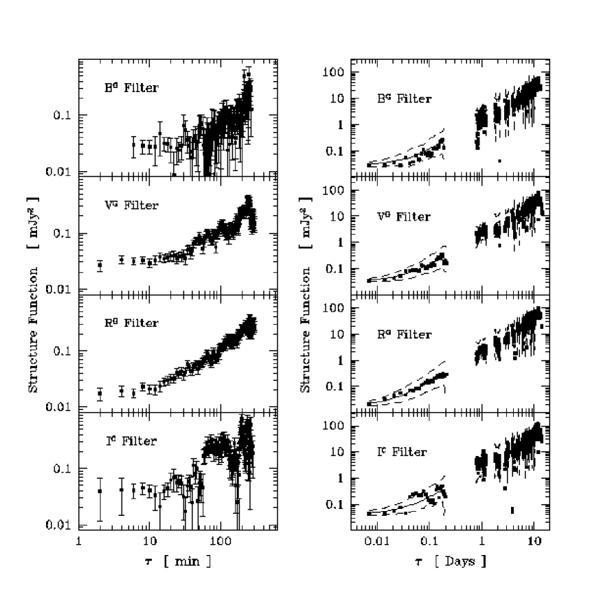
Fig. 5.: a and b. Structure functions of the B_G, V_G, R_G, and I_C light curves: a SFs for very short $\tau$, with $\delta=5$ min. b SFs for long $\tau$, with $\delta=10$ min. The solid lines are the mean SFs of the simulated light curves, and the dashed lines show the $\pm 1\penalty 10000\kern 3.0pt\sigma$ limits. The SF of the U_G light curve has not been calculated because of the very poor sampling

In the case of the Fourier transform, the effects of a bad sampling are important, but they can be formulated in an analytical way, and, in the most fortunate cases, properly corrected using a deconvolution. For the SF, we do not have such a knowledge about the perturbations introduced by the sampling. But because of the particular sampling we have obtained, we expect that they will be much smaller than in the case of the Fourier transform. Indeed, for some values of $\tau$, e.g. 0.5, 1.5, 2.5,…days, the SF will be completely unknown, because no observation can be performed 12 hours after an observation with a single ground-based optical telescope. On the other hand, for some values of $\tau$, e.g. 0.1, 1.0, 2.0,…days, the number of couples per bin will be very large, and should lead to a very good determination of the SF. Thus, by preferring the SF approach, we concentrate the information in some parts of the SF, instead of spreading it over the complete Fourier domain.

The SFs of the B_G, V_G, R_G, and I_C light curves are shown in Fig.5. The SF of the U_G light curve has not been calculated, because of the very small number of observations in this filter. Two main features can be observed in the SFs. The first feature is the presence of a horizontal branch at short $\tau$. This is due to the fact that the variability of the time series on very short time scales is dominated by the white noise introduced by the measurement errors on the fluxes. As the amplitude of a white noise is independent of the lag between the two observations, the SF of a pure white noise process is constant, with a value equal to twice the variance of the white noise. Thus the SF at very short $\tau$ gives an experimental estimation of the uncertainties on the flux, $\varepsilon_{\mathrm{SF}}$. These are given in Table1. The R_G light curve, which has the largest accuracy, shows variability on time scales as short as 15 min ($0.01$ days).

The second feature is a roughly linear increase of the logarithms of the SFs with $\log\tau$ with a slope about 1.3. An important property of the SF is that the SF of a time series whose Fourier power spectrum follows a power-law also follows a power-law. As a first approximation, we assume that the light curves have power-law shaped Fourier power spectra. As we cannot correct our SFs from the effect of the sampling, we use the opposite approach: we simulate 100 continuous time series whose Fourier power spectra follow a power-law with different indices. To construct the time series, we simply add together sine functions with random phases, with the constraint that the power in each frequency bin decreases as specified. This is a discrete approximation of a continuous process, but, owing to the very large number of sine functions added together, we expect that no serious discrepancy will result from this method. We then project the simulated light curves onto the sampling obtained for the different filters, and calculate their SFs. As a result, we obtain the mean SF for our sampling of a light curve that is characterized by a power-law-shaped Fourier power spectrum with a specified index.

The power-spectrum index that matches most closely the observed SFs of the 4 light curves is $-2.4$, the indices between $-2.2$ and $-2.7$ being acceptable (we normalized the simulated light curves so that their standard deviation are identical to the one of the observed light curves; therefore the SFs of the simulated light curves match the one of the real light curve at large $\tau$ for all indices). We can also remark that the features in the SF of the light curves (e.g. the relative drop around $\tau\sim$ 2 days) are not at all significant when one considers the dispersion in the SFs of the simulated light curves.

5 Delay between the light curves

The existence of a delay between the light curves at different wavelengths is an important issue, since it has implications on the emission mechanism. We test this point using two methods.

5.1 Cross-correlation

The cross-correlation is the most standard way to obtain a lag between two time series. We use the interpolated correlation function (ICF) introduced in ?). This method is more appropriate to our sampling than the discrete correlation function ?, provided that we calculate the correlations for lags smaller than 0.2 days. The reason is that the interpolation between two observations made during the same night is a very good approximation of the actual flux, because of the small amplitude of variability for very short lags (see Sect.4). Note that ?) have found that the ICF method was more efficient than the DCF one when dealing with simulated flaring light curves.

Fig. 6.: ICF correlation between the R_G and the B_G light curves (solid line). The dashed line is the fit by a Gauss profile. Its centre is indicated by a dotted line at $\tau=-44.8$ min

The cross-correlations of the different light curves with the V_G and R_G light curves obtained with the ICF method all show a very broad peak that we fitted with a Gauss profile to find its centre (Table2 and Fig.6). The peak values are in all cases very close to 1, which indicates an excellent correlation. It appears that the shorter wavelengths are leading the longer ones. To check whether we have really detected a lag, we use the set of 100 simulated light curves with an index $-2.4$ described in Sect.4, that we projected onto the samplings of the real light curves. About 10% of the correlations produced a central peak that could not be fitted by a Gauss profile. This produced aberrant values for the location of the correlation peak. Instead of analyzing each of these correlations to obtain a correct value for the lag, we simply discarded all the values of the lag outside the range $[-0.1;0.1]$ days. The distribution of the remaining lags is compatible with a Gauss distribution. The statistics of the location of the peaks are given in Table2. As the dispersions of the distributions are about 8 times smaller than the width of the domain where we considered the lags as valid, we can conclude that the rejection of the values out of the domain is justified. The mean lags of the simulations are different from 0, but significantly smaller than the dispersion, and are thus neglected. Fig.7 shows the results of the cross-correlation analysis. The significances of the individual lags are small ($<2\sigma$). However two points indicate that the lags are most probably real. First, the lag increases monotonously from the B_G to the I_C filters. The probability that this happens by chance is the probability to obtain a 100% correlation with a Spearman’s test on 4 points, which is about 2%. Moreover, this has been realized twice independently, since the same observation can be made for the lags with the R_G light curve. The second point is that the lags between the B_G light curve and the V_G and R_G light curves are compatible. This is also true for the lags between the I_C light curve and the V_G and R_G light curves.

Table 2.: Results of the cross-correlations of the observed and simulated light curves. A negative lag means that the second light curve is leading. The last two columns refer to the simulated light curves

Filters	Observed lag	Mean lag	Dispersion
	(min)	(min)	(min)
VG–BG	–28.2–	+14.7	37.9
VG–RG	43.5	–09.5	36.9
VG–IC	58.2	–01.4	32.3
RG–BG	–44.8–	+12.7	40.4
RG–IC	23.2	+07.0	38.2

Table 3.: Results of the global $\chi^{2}$ minimization. A negative lag means that the second light curve is leading. The “significance” is the departure from a zero lag in units of the standard deviation for the assumptions $\Delta\chi^{2}=1$ and $\Delta\chi^{2}=2.5$

Filters	Lag	Best $\chi^{2}/$	$\Delta\chi^{2}=$		Significance
	(min)	d.o.f.	1	2.5	1	2.5
VG–BG	–14.4	403.6/371	$\left({}^{+4.3}_{-5.8}\right)$	$\left({}^{+7.9}_{-9.4}\right)$	3.3	1.8
VG–RG	–18.7	563.9/485	$\left({}^{+3.2}_{-3.2}\right)$	$\left({}^{+4.7}_{-5.0}\right)$	5.8	4.0
VG–IC	–22.3	486.2/391	$\left({}^{+6.5}_{-4.3}\right)$	$\left({}^{+8.6}_{-7.2}\right)$	3.4	2.6

Fig. 7.: Lag between the light curves. The black squares are the lags with the V_G light curves (the dotted line is the zero lag line). The error bars are the dispersions of the lag in the simulations. The black triangles are the analogous of the black squares, but with respect to the R_G light curves, except that a lag of $43.5$ min has been added (the lag between the V_G and the R_G light curves). The dashed line is the zero lag line for the R_G light curve. The empty circles are the results of the global $\chi^{2}$ minimization method, and give the lag with the V_G light curve. The thick error bars correspond to $\Delta\chi^{2}=1$, and the thin ones to $\Delta\chi^{2}=2.5$

5.2 Global $\chi^{2}$ minimization

The global $\chi^{2}$ minimization method has been introduced by ?) to determine the delay between two images of a gravitationally-lensed quasar. The principle of the method is as follows: Assuming two unevenly-sampled time series $(t^{\mathrm{x}}_{i},x_{i}),\penalty 10000\kern 3.0pti=1,\ldots,n$ and $(t^{\mathrm{y}}_{j},y_{j}),\penalty 10000\kern 3.0ptj=1,\ldots,m$, we concatenate them to form a new time series $(t^{\mathrm{z}}_{\tau_{0},i},z_{\tau_{0},i}),\penalty 10000\kern 3.0pti=1,\ldots,n+m$, one of the two time series being shifted in time by an arbitrary lag $\tau_{0}$. If the covariance properties of the initial time series are known, one can check whether the concatenated time series has the same covariance properties. This can be made by calculating:

$$\chi^{2}=(z_{\tau_{0}}-\alpha\mathchoice{\mbox{$\mathbf{\displaystyle E}$}}{\mbox{$\mathbf{\textstyle E}$}}{\mbox{$\mathbf{\scriptstyle E}$}}{\mbox{$\mathbf{\scriptscriptstyle E}$}})^{T}\penalty 10000\kern 3.0pt(\mathchoice{\mbox{$\mathbf{\displaystyle C}$}}{\mbox{$\mathbf{\textstyle C}$}}{\mbox{$\mathbf{\scriptstyle C}$}}{\mbox{$\mathbf{\scriptscriptstyle C}$}}^{-1})\penalty 10000\kern 3.0pt(z_{\tau_{0}}-\alpha\mathchoice{\mbox{$\mathbf{\displaystyle E}$}}{\mbox{$\mathbf{\textstyle E}$}}{\mbox{$\mathbf{\scriptstyle E}$}}{\mbox{$\mathbf{\scriptscriptstyle E}$}}),$$ (3)

where $\mathbf{\textstyle C}$ is the total covariance matrix of the process (including measurement noise), in analogy with the usual $\chi^{2}$ definition: $\chi^{2}=\sum_{i=1}^{n}\penalty 10000\kern 3.0pt(x_{i}/\sigma_{i})^{2}$. The term $z-\alpha\mathchoice{\mbox{$\mathbf{\displaystyle E}$}}{\mbox{$\mathbf{\textstyle E}$}}{\mbox{$\mathbf{\scriptstyle E}$}}{\mbox{$\mathbf{\scriptscriptstyle E}$}}$ mean that we subtract a constant $\alpha$ to all components of the $z_{\tau_{0}}$ vector ($\mathbf{\textstyle E}$ is the vector unity). $\alpha$ is the value that minimizes the $\chi^{2}$ in the above equation for an assumed lag, and is given by:

$$\alpha=\frac{\mathchoice{\mbox{$\mathbf{\displaystyle E}$}}{\mbox{$\mathbf{\textstyle E}$}}{\mbox{$\mathbf{\scriptstyle E}$}}{\mbox{$\mathbf{\scriptscriptstyle E}$}}^{T}\penalty 10000\kern 3.0pt(\mathchoice{\mbox{$\mathbf{\displaystyle C}$}}{\mbox{$\mathbf{\textstyle C}$}}{\mbox{$\mathbf{\scriptstyle C}$}}{\mbox{$\mathbf{\scriptscriptstyle C}$}}^{-1})}{\mathchoice{\mbox{$\mathbf{\displaystyle E}$}}{\mbox{$\mathbf{\textstyle E}$}}{\mbox{$\mathbf{\scriptstyle E}$}}{\mbox{$\mathbf{\scriptscriptstyle E}$}}^{T}\penalty 10000\kern 3.0pt(\mathchoice{\mbox{$\mathbf{\displaystyle C}$}}{\mbox{$\mathbf{\textstyle C}$}}{\mbox{$\mathbf{\scriptstyle C}$}}{\mbox{$\mathbf{\scriptscriptstyle C}$}}^{-1})\penalty 10000\kern 3.0pt\mathchoice{\mbox{$\mathbf{\displaystyle E}$}}{\mbox{$\mathbf{\textstyle E}$}}{\mbox{$\mathbf{\scriptstyle E}$}}{\mbox{$\mathbf{\scriptscriptstyle E}$}}}\penalty 10000\kern 3.0ptz_{\tau_{0}}$$ (4)

It has the purpose of eliminating the bias introduced by the fact the both the mean and the variance measured in our data are usually different from their real values. This correction even allows us to use the method for low-frequency-divergent time series.

The covariance matrix is constructed on the basis of the most complete structure function drawn as a solid line in Fig.5b; it is important to notice that this covariance matrix is very well constrained by our data. The details of the construction of this matrix are to be found in ?) and ?). A drawback of the method is that it works only if the $x_{i}$ and $y_{i}$ data are two realizations of the same time series, apart from the existence of a lag, and a possible difference in mean value. We therefore have to transform the flux in one filter into the flux that we would have observed in the other filter. We have observed that the flux in a given filter can be very well approximated by a constant term plus a linear function of the flux in another filter, all the correlation coefficients being larger than 0.995.

The delay is then obtained by minimizing $\chi^{2}(\tau_{0})$. The results are given in Table3, and are plotted on Fig.7. We see that the lags are essentially consistent with the ones found with the ICF method. As it does follow a real $\chi^{2}$ statistics, we can in principle estimate the uncertainties on $\tau_{0}$ by the condition $\Delta\chi^{2}=1$. However ?) used the $\Delta\chi^{2}=2.5$ after running a set of Monte-Carlo simulations. As the computation time is huge, we did not try to find the uncertainties on the lags with our simulated light curves. But, contrarily to the situation encountered by ?), the values of the lag that we have found are in the range where the method should work well; therefore we believe that the $\Delta\chi^{2}=2.5$ assumption is very conservative. The uncertainties are in any case much smaller than in the previous case. The significances are quite high for all the lags, even if one uses the conservative assumption.

The probability to obtain such $\chi^{2}$ values are respectively 12%, 0.8%, and 0.07%. The last two values are very improbable. This may be due to the fact that this method compares only identical time series. We used experimental relationships to transform the fluxes in the filters into “equivalent V_G fluxes”. This can explain easily the high $\chi^{2}$ values.

6 Discussion

Emission of BL Lac objects is generally supposed to originate from synchrotron radiation (at least at low frequency). Other mechanisms for variability have been proposed, like gravitational micro-lensing or geometrical variations. We are not going to compare detailed models with the results obtained here, because of their complexity and of the number of free parameters involved. However our results are strong enough to constrain the qualitative properties of the models.

6.1 Time-series properties of the light curves

We have obtained a very good description of the Fourier power spectra of the optical light curves of PKS 2155-304. We can check the compatibility of our result with the observations from the 1991 campaign. Fig.8 shows the two SFs of the V (considered identical to V_G) light curve from the 1991 campaign and of our V_G light curves. We see that both SFs are compatible, apart from the effect of the measurement white noise, which has an amplitude 10 times lower in our data. This comparison may indicate that the light curves of PKS 2155-304 are stationary time series, or at least that the spectral properties observed in the present campaign are not completely peculiar.

Another comparison can be made with the result of ?). They found that the Fourier power spectrum of EXOSAT observations of PKS 2155-304 follows a power-law with an index $-2.5\pm 0.2$, fully compatible with our result. Even after the removal of the linear trend, the index ($-1.9\pm 0.4$) is still compatible with our result. This shows that the X-ray and optical emission are strongly related, and that they have probably the same origin. However, even in this case, many models predict that the optical power spectrum will decrease more rapidly than the X-ray one, the short-time scale variability being attenuated at large wavelength, mostly because of the longer cooling time (e.g., in synchrotron radiation). This is not observed in our campaign. These effects, if they exist, must take place on time scales even shorter than those investigated here, i.e. about 15 min. At least down to this limit, variability is produced by a wavelength-independent mechanism, for instance geometrical. This possibility will be rediscussed below.

6.1.1 Power-spectrum at very high frequencies

The structure functions of Fig.5 are all dominated by the white noise introduced by the measurement uncertainties for $\tau<10$ min. It means that we can only put an upper limit to the minimum variability time scale in this object. In addition, the structure function analysis tells us that, if the time between two consecutive observations is $\tau_{0}$, the variability in the V_G band from the first observation to the second one is:

$$\sigma_{\tau_{0}}\simeq\left(\frac{1.4\cdot 10^{-4}}{2}\cdot\tau_{0}^{1.3}\right)^{1/2}\mbox{\penalty 10000\kern 3.0ptmJy},$$ (5)

where $\tau_{0}$ is expressed in min. The accuracy should be of the order 0.02 mJy, i.e. 0.1 % of the flux, to detect variability on time scales of 5 min. The above formula can help in the planning of future missions aiming at probing the smallest variability time scale in PKS 2155-304. Although very-short-term variability does exist in PKS 2155-304, its amplitude is very low. This is due to the steepness of the power spectrum.

6.1.2 Power-spectrum at very low frequencies

Fig. 8.: Structure functions of the light curves in the V band from our campaign (black squares), the 1991 campaign (crosses), the Harvard data set (empty squares), and the complete photographic data set (black circles). The solid line is a power-law with an index $1.3$ with a break around 20 days and a contamination with a white noise with a standard deviation of 0.13 mJy. The dashed line is the same power-law, but contaminated by a white noise with a standard deviation of 1.34 mJy. This clearly shows the increase of the accuracy reached in our campaign

As our campaign lasted only 15 days, it is impossible to investigate the existence of time scales longer than this duration. However there exists many other observations that can be used to determine the complete power spectrum. We have used the data from ?). The observations are photographic plates that have been converted into B magnitudes. Their data are presented in two separate sets: a first set contains the data from the Harvard photometric collection; it spans about 2 500 days and contains 66 observations. The second one contains all photographic observations, but the data have been averaged by year; the set spans about 90 years and contains 44 annual averages. The B magnitudes have been transformed into fluxes using a 0-mag flux of $4.27\cdot 10^{6}$ mJy. To transform the variations into variations in the V band, we transformed the B fluxes into V_G fluxes using the linear relationship that we have found between the B_G and V_G fluxes.

The SFs of the Harvard data set and of the complete photographic data set are also plotted. The uncertainties on theses SFs are large, because of the poorness of the sampling, but we see that the SFs of the two long-term data sets do not follow the increase seen in the present campaign. As the complete data set is averaged by year, one must consider its SF as a underestimation of the real SF, because such an average has great chances of reducing the variability. Taking this point into account, this SF is compatible with the SF of the Harvard data. The tentative SF drawn on Fig.8 indicates that the longest variability time scales in PKS 2155-304 lies between 10 and 40 days, apart perhaps from time scales longer than 100 years.

6.1.3 Origin of the power spectrum

The variability of PKS 2155-304 is small, and the light curves are very different from what is observed in, for instance, OJ 287 ?, which has an amplitude of variability of at least 4 mag, i.e. a factor 40. Actually the variability of OJ 287 appears in sudden bright “flares”, which could show that the mechanisms that produce the essential of the variability are very different from those at work in PKS 2155-304 ?. Apart from the distinction between “flaring” and “non-flaring” objects, we do not know whether the Fourier properties of PKS 2155-304 are typical of BL Lac objects. We have indeed here the most extensive (in term of spectral coverage) study of the power spectrum of any active galactic nucleus. The most important point is that all the data are compatible with a power-law-shaped power spectrum with an index $-2.4$, and and low-frequency cut-off at frequencies as high as (10-40 days)^-1.

Many other time series in the physical world have a power-law-shaped Fourier spectrum ?, but no convincing physical mechanism has ever been proposed ?. Several physical processes have been proposed for X-ray light curves of Seyfert galaxies. The underlying idea of most of them can be formulated by the “mechanical model” of ?). He has shown analytically that a superimposition of any “reasonable” (as defined in his paper) time-dependent perturbations with different time scales and amplitude can generate any spectral index in the Fourier domain. As our index is smaller than $-2$, it means that we can constrain the properties of the perturbations. It requires indeed that the Fourier power spectrum of the perturbations decreases with an index at most $-2.4$. Therefore exponential pulses, whose Fourier power spectrum decreases with an index $-2$, are excluded. A candidate for the events could be the injection of packets of relativistic electrons, which cool by emitting synchrotron radiation. Variations in the parameters of the packets (size, energy distribution of the electrons, …) could produce the diversity of amplitudes and time scales required to obtain a power-law-shaped Fourier spectrum (but see Sect.6.2 for the problem of spectral index variation). In this case the low-frequency cut-off is related to the maximum cooling time of the packets, if the “birth times” of the packets are completely independent from each other.

Another possibility of producing a power-law-shaped Fourier spectrum is by summing many periodic functions with different periods. Following the idea of ?), a “knot” can have a helical motion around the magnetic field, which produces periodic flares, because of the periodic variation of the Doppler amplification towards the observer. A large enough number of knots with different gyration radii could fill the power spectrum to produce a power-law. ?) found that the typical time scales induced around a $10^{8}$ M_⊙ black hole should be of the order of 1 day. However it seems plausible that smaller time scales can be obtained with modifications of the geometry of the system, like the angle between the jet and the observer, the velocity of the knot, or the mass of the black hole.

We can further add that it seems rather improbable to us that gravitational micro-lensing can explain the light curves observed in our campaign. Even though ?) have shown that the light curves generated by a micro-lensing foreground galaxy can be very complex and have broad Fourier power spectra, their shapes show successions of sharp flares, which do not appear in the light curves from this campaign or from the 1991 campaign (1991-I, 1991-II, 1991-III).

Because variability is essentially geometrical (provided that the cooling times of the packets are significantly longer that the time scale of the geometrical variability), these last two models predict a power spectrum mostly independent of the frequency, as observed.

6.2 Spectral behaviour of PKS 2155-304

A correlation between spectral index and flux is clearly seen in our data. It has however not always been the case in other studies on PKS 2155-304. CCD optical observations from ?) indicate that there is no correlation between the B-V colour index and the V magnitude. The complete archive of IUE spectra shows that the variability increases when the wavelength decreases ?, but ?) found using a large part of this archive that the flux and the spectral index were not correlated. On the other hand he found a (not very clear) correlation in MRK 421. In the 1991 campaign the constant spectral index hypothesis was favoured in the optical data (1991-III), while a hardening of the spectrum when the source brightens was the general behaviour observed in the ultraviolet domain ?, but the details were very complex and do not support the clear correlation found in our data. In other BL Lac objects, the correlation has been found to be very significant (e.g., OJ 287: ? ?; AO 0235+164, PKS 0735+178, 1308+326: ? ?). On the other hand, in a study of 6 BL Lac objects, ?) found only two cases of positive correlations.

Examining Fig.4, it appears that the spectral index is compatible with a constant as soon as the flux in the V_G band is larger than 18 mJy. An explanation for the drop of spectral index at low fluxes could be that the fluxes are contaminated by a constant emission, e.g. from the host galaxy, that is fainter and steeper than the BL Lac component. PKS 2155-304 was rather weak during this campaign. Indeed the mean V flux obtained here is about 15 % smaller than the one obtained during the 1991 campaign. Moreover the V flux was below 18 mJy during about the half of the campaign, while it was below this value during about only 20 % of the 1991 campaign. This, together with the much better signal-to-noise ratio obtained in our campaign, could explain why the drop of the spectral index at small flux has not been observed during the 1991 campaign. A further argument in favour of the existence of an underlying component comes from the remark made in Sect.5.2: The best way that we have found to transform a flux into a V_G flux is through a linear relationship with a constant that increases with the wavelength; a comparable observation in Seyfert galaxies has been interpreted by ?) as the signature of an underlying component. Therefore we cannot exclude the possibility of a constant (or weakly varying) spectral index, and it is the interpretation that we favour.

A few optical observations from the 1991 campaign are in disagreement with the above interpretation that the variations are achromatic (apart from the existence of an underlying component). It is also the case for several of the campaigns on PKS 2155-304 cited above. However in the two optical campaigns, most of the observations are compatible with the constant spectral index hypothesis (note that a drop of the colour index can be marginally observed in ?)). It suggests that the variability is mostly achromatic (or weakly chromatic), with some casual significant excursions of the spectral index from the average value.

Achromatic variability cannot be easily accounted for in terms of synchrotron radiation, because it would require a very fine tuning between injection terms and electron losses. On the other hand small variations of the angle between the jet and the observer, or of the bulk Lorenz factor can generate achromatic variability. Gravitational micro-lensing by the stars of a foreground galaxy has already been invoked to explain the variability of BL Lac objects ??. However, as mentioned above, variability is not really achromatic, but rather the spectral index has little variations, which are uncorrelated with the flux. This cannot be easily explained either by geometrical variations alone or by micro-lensing. As the flux variability is rather small, it may be that spectral index variation is small, if a large number of packets of electrons with different energy distributions participate in the optical emission. Moreover a campaign performed in May 1994 that included ASCA observations showed that the variability in the hard X-ray domain (above the range covered by ROSAT in 1991-II) was quite different both in amplitude and in time scales from what has been observed with IUE ?.

6.3 Delay between the light curves

In 1991-IV, ? already observed a lag of 2–3 hours between the ROSAT X-ray light curve and the IUE 1400 Å light curve. We confirm the existence of lags between the different wavelengths, in the sense that the light curves at shorter wavelengths lead the light curves at longer wavelengths. The delays between the optical light curves are about 40 min for a factor 2 in frequency. This value is actually very close (and compatible, owing to the large uncertainties on these values) to the amplitude of the lag between the ROSAT X-ray light curve and the IUE 1400 Å light curve (a factor $\sim 50$ in frequency).

Inhomogeneous jets, i.e. where electrons are injected at the base of the jet and emit most of the synchrotron radiation at frequencies decreasing with the distance to the base, naturally produce a lag in the sense observed here (but see Sects6.2 and 7). It has however been noted in 1991-IV that the amplitude of the X-ray–ultraviolet lag is inconsistent with models where electrons are injected and not reaccelerated, because the life time of a X-ray-emitting electron is extremely short (of the order of the second in the model of ?)). The problem also exists in the optical domain, where the lag is comparable to the one between the X-ray and the ultraviolet emissions, and the life time of the optical-emitting electrons has only increased by a factor of the order of 10.

This problem can be solved if the lag is due to a bubble of electrons that becomes progressively optically thin at longer wavelengths ?. We note however that we disagree with the observation made in 1991-IV that the lag is shorter than the shortest variability time scales. The 2–3 hours observed in the X-ray domain are at least 8 times longer that the shortest variability time scale observed in the R_G light curves, and assuredly only the measurement noise has prevented us to detect even shorter time scales. This is difficult to explain with this model.

Although stated in the literature (e.g., 1991-IV), we do not consider plausible that gravitational micro-lensing models can account for the existence of a lag. The mechanism proposed in 1991-IV should produce a broad, but symmetrical with respect to $\tau=0$, correlation peak.

Note that the presence of lag between two light curves automatically implies spectral-index variation. In PKS 2155-304, the short-time scale variability is sufficiently small, so that the variation of the spectral index due to the lag remains undetected.

7 Summary and conclusion

7.1 Results on the variability of PKS 2155-304

We have performed several types of analyses to extract the physical properties of the optical light curves of PKS 2155-304. The main results are the followings:

1. The structure function of the optical variability is compatible with the one expected for a power-law-shaped Fourier power spectrum with an index $-2.4$.

2. The shortest variability time scale observed is about 15 min, but it is an upper limit, as the variability is dominated by the measurement white noise below this time scale.

3. The optical spectrum hardens when the source brightens. We conclude however that this is probably due to an underlying stable component. As a consequence the variability of the BL Lac component in PKS 2155-304 is considered to be achromatic during this campaign.

4. The fluxes at different wavelengths are very well correlated.

5. There is a lag between the different light curves. The light curves at longer wavelengths are delayed with respect to the light curves at shorter wavelengths. The amplitude of the delay is about 40 min for a factor 2 in frequency.

To these results, we can add those obtained from the comparison with other data:

1. The maximum variability time scale is comprised between 10 and 40 days. There is no evidence of variability on time scales between 40 days and 100 years.

2. The shapes of the power spectra in the optical and X-ray domain are compatible.

3. The optical spectral index has been observed to vary slightly without correlation with the flux during other campaigns.

4. The lag between the X-ray and the ultraviolet light curves is 2-3 hours for a factor 50 in frequency, i.e. 20-30 min for a factor 2 in frequency, which is very close to the lag in the optical domain.

7.2 General conclusions

We have considered the global properties of several models that could explain the variability of PKS 2155-304: synchrotron radiation from an inhomogeneous jet ?, synchrotron radiation from an shocked bubble ?, variability induced by geometrical variations ?, and variability induced by gravitational micro-lensing events ??. The following conclusions can be drawn from the above results. They are sufficiently general to be independent of the details of the models.

Power spectrum origin

Points (1), (2), and (6) give a very complete knowledge of the variability properties of the optical light curve. The meaning of the low- and high-frequency limits of the power spectrum cannot be understood without a knowledge of the variability mechanism. This is also true for the shape of the power spectrum. But we can exclude models where the light curve is generated by the sum of a large number of exponential pulses, while other shapes of pulses are fully viable. We can moreover note that some models are less susceptible of generating the kind of light curves and power spectra observed here, in particular this seems to be the case for the micro-lensing model.

Power spectrum constancy

Points (4), and (7) indicate that, if the optical power spectrum got through a high-frequency filter, the low-frequency cut-off of this filter would be at very high frequencies ($>\!(0.01\mbox{\penalty 10000\kern 3.0ptdays})^{-1}$). We prefer another explanation, namely that the high-frequency variability has a geometrical origin.

Gravitational micro-lensing models

can be ruled out by Points (3), (4), and (5): Point (3) indicates that the size of the blue-light emitting region is the same that the one of the near-infrared-light emitting region, but Point (5) shows that these regions cannot be identical, and Point (4) would imply that all lenses cross first the blue-light emitting region, and about one hour later the near-infrared-light emitting region with the same amplification parameters. This is, of course, extremely improbable.

Amplitude of the lag

Points (5), and (9) show that the lag observed between the light curves is much larger than the one predicted by inhomogeneous jet models without reacceleration. A model in which a dense bubble subject to synchrotron self-absorption becomes progressively optically thin can however explain this lag.

Lag – variability time scale problem

We must remark that Points (3), (4), and (5) are difficult to reconcile for any model. Models where variability is “geometrical” can account for the achromaticity of the optical variability, but it appears difficult to explain a lag significantly longer than the minimum variability time scale. This favours an interpretation where low- and high-frequency variabilities have different origins (e.g. synchrotron cooling and geometrical variations respectively).

(Quasi-)achromaticity of the light curves

Synchrotron emission does not naturally produce achromatic variations, as observed in Point (3). If synchrotron radiation is the mechanism that produces the optical emission of PKS 2155-304, the slight spectral index variations (Point (8)) make us think that the optical emission is produced by a number of bubbles sufficiently large to “dilute” efficiently the spectral index variations induced by each bubble.

The variability picture of PKS 2155-304 remains a very difficult puzzle, but the results given in this paper are very constraining. To our mind, the most interesting issue raised here is to find a mechanism that can explain simultaneously important lags and well-correlated variability on very short time scales. But we keep also in mind that other events not described here, because not observed during this campaign, exist in PKS 2155-304, like the ASCA flare ?.

• SP acknowledges a grant from the Swiss National Science Foundation.

References

- Blecha etal.(1990)Blecha, Weber, Simond & Queille BlechaA., WeberL., SimondG. & QueilleD., 1990. In: JacobyG.H.(ed.), CCDs in Astronomy, ASP Conference Series8, p. 192
- Brinkmann etal.(1994)Brinkmann, Maraschi, Treves, Urry, Warwick, Siebert, Wagner, Edelson, Fink & Madejski BrinkmannW., MaraschiL., TrevesA., etal., 1994, A&A288, 433 – 1991-II
- Brown etal.(1989)Brown, Robson, Gear, Hughes, Griffin, Geldzahler, Schwartz, Shepherd, Webb, Valtaoja, Terasranta & Salonen BrownL.M.J., RobsonE.I., GearW.K., etal., 1989, ApJ340, 129
- Camenzind & Krockenberger(1992) CamenzindM. & KrockenbergerM., 1992, A&A255, 59
- Courvoisier etal.(1995)Courvoisier, Blecha, Bouchet, Bratschi, Carini, Donahue, Edelson, Feigelson, Filippenko, Glass, Heidt, Kollgaard, Matheson, Miller, Noble, Sekiguchi, Smith, Urry & Wagner CourvoisierT.J.-L., BlechaA., BouchetP., etal., 1995, ApJ438, 108 – 1991-III
- Edelson(1992) EdelsonR., 1992, ApJ401, 516
- Edelson etal.(1995)Edelson, Krolik, Madejski, Maraschi, Pike, Urry, Brinkmann, Courvoisier, Ellithorpe, Horne, Treves, Wagner, Wamsteker, Warwick, Aller, Aller, Ashley, Blecha, Bouchet, Bratschi, Bregman, Carini, Celotti, Donahue, Feigelson, Filippenko, Fink, George, Glass, Heidt, Hewitt, Hughes, Kollgaard, Kondo, Koratkar, Leighly, Marscher, Martin, Matheson, Miller, Noble, O’Brien, Pian, Reichert, Saken, Shull, Sitko, Smith, Sun & Tagliaferri EdelsonR., KrolikJ., MadejskiG., etal., 1995, ApJ438, 120 – 1991-IV
- Edelson & Krolik(1988) EdelsonR.A. & KrolikJ.H., 1988, ApJ333, 646
- Edelson etal.(1991)Edelson, Saken, Pike, Urry, George, Warwick, Miller, Carini & Webb EdelsonR.A., SakenJ., PikeG., etal., 1991, ApJ372, L9
- Gaskell & Peterson(1987) GaskellC.M. & PetersonB.M., 1987, ApJS65, 1
- Gear etal.(1986)Gear, Robson & Brown GearW.K., RobsonE.I. & BrownL.M.J., 1986, Nat324, 546
- Ghisellini etal.(1985)Ghisellini, Maraschi & Treves GhiselliniG., MaraschiL. & TrevesA., 1985, A&A146, 204
- Griffiths etal.(1979)Griffiths, Briel, Chaisson & Tapia GriffithsR.E., BrielU., ChaissonL. & TapiaS., 1979, ApJ234, 810
- Halford(1968) HalfordD., 1968, Proc. IEEE56, 251
- Kayser etal.(1989)Kayser, Refsdal, Weiss & Schneider KayserR., RefsdalS., WeissA. & SchneiderP., 1989, A&A214, 4
- Litchfield etal.(1995)Litchfield, Robson & Hughes LitchfieldS.J., RobsonE.I. & HughesD.H., 1995, A&A300, 385
- Marscher & Gear(1985) MarscherA.P. & GearW.K., 1985, ApJ298, 114
- Massaro & Trevese(1996) MassaroE. & TreveseD., 1996, A&A312, 810
- Massaro etal.(1995)Massaro, Nesci, Perola, Lorenzetti & Spinoglio MassaroE., NesciR., PerolaG.C., LorenzettiD. & SpinoglioL., 1995, A&A299, 339
- Miller & Carini(1991) MillerH.R. & CariniM.T., 1991. In: MillerH.R. & WiitaP.(eds), Variability of AGN, p. 111, CUP
- Paltani & Courvoisier(1994) PaltaniS. & CourvoisierT.J.-L., 1994, A&A291, 74
- Paltani & Walter(1996) PaltaniS. & WalterR., 1996, A&A312, 55
- Paltani etal.(1996)Paltani, Courvoisier, Bratschi & Blecha PaltaniS., CourvoisierT.J.-L., BratschiP. & BlechaA., 1996. In: MillerH.R., WebbJ.R., & NobleJ.C.(eds), Blazar Continuum Variability, ASP Conference Series 110, p.36
- Press(1978) PressW.H., 1978, Comm. Astroph.7, 103
- Press etal.(1992)Press, Rybicki & Hewitt PressW.H., RybickiG.B. & HewittJ.N., 1992, ApJ385, 404
- Racine(1970) RacineR., 1970, ApJ159, L99
- Rufener & Nicolet(1988) RufenerF. & NicoletB., 1988, A&A206, 357
- Rutman(1978) RutmanJ., 1978, Proc. IEEE66, 1048
- Rybicki & Press(1992) RybickiG.B. & PressW.H., 1992, ApJ398, 169
- Schneider & Weiss(1987) SchneiderP. & WeissA., 1987, A&A171, 49
- Sillanpää etal.(1996)Sillanpää, Takalo, Pursimo, Lehto, Nilsson, Teerikorpi, Heinaemaeki, Kidger, De Diego, Gonzalez-Perez, Rodriguez-Espinosa, Mahoney, Boltwood, Dultzin-Hacyan, Benitez, Turner, Robertson, Honeycut, Efimov, Shakhovskoy, Charles, Schramm, Borgeest, Linde, Weneit, Kuehl, Schramm, Sadun, Grashuis, Heidt, Wagner, Bock, Kuemmel, Heines, Fiorucci, Tosti, Ghisellini, Raiteri, Villata, De Francesco, Bosio & Latini SillanpääA., TakaloL.O., PursimoT., etal., 1996, A&A305, L17
- Simonetti etal.(1985)Simonetti, Cordes & Heeschen SimonettiJ.H., CordesJ.M. & HeeschenD.S., 1985, ApJ296, 46
- Tagliaferri etal.(1991)Tagliaferri, Stella, Maraschi, Treves & Celotti TagliaferriG., StellaL., MaraschiL., TrevesA. & CelottiA., 1991, ApJ380, 78
- Urry(1996) UrryC.M., 1996. In: MillerH.R., WebbJ.R., & NobleJ.C.(eds), Blazar Continuum Variability, ASP Conference Series 110, p. 391
- Urry etal.(1993)Urry, Maraschi, Edelson, Koratkar, Krolik, Madejski, Pian, Pike, Reichert, Treves, Wamsteker, Bohlin, Bregman, Brinkmann, Chiappetti, Courvoisier, Filippenko, Fink, George, Kondo, Martin, Miller, O’Brien, Shull, Sitko, Szymkowiak, Tagliaferri, Wagner & Warwick UrryC.M., MaraschiL., EdelsonR., etal., 1993, ApJ411, 614 – 1991-I
- Voss & Clarke(1975) VossR.F. & ClarkeJ., 1975, Nat258, 317
- Wagner & Witzel(1995) WagnerS.J. & WitzelA., 1995, ARA&A33, 163
- Weber(1993) WeberL., 1993, Inter – Manuel de référence, Observatoire de Genève
- Zhang & Xie(1996) ZhangY.H. & XieG.Z., 1996, A&AS116, 289