Measuring Cosmological Parameters with Galaxy Surveys

Abstract

We assess the accuracy with which future galaxy surveys can measure cosmological parameters. By breaking parameter degeneracies of the Planck Cosmic Microwave Background satellite, the Sloan Digital Sky Survey may be able to reduce the Planck error bars by about an order of magnitude on the large-scale power normalization and the reionization optical depth, down to percent levels. However, pinpointing attainable accuracies to within better than a factor of a few depends crucially on whether it will be possible to extract useful information from the mildly nonlinear regime.

]

I INTRODUCTION

One of the main challenges in modern cosmology is to refine and test the standard gravitational instability model of structure formation by precision measurements of its free parameters: the slope $n$ and normalization $Q$ of the primordial spectrum of density fluctuations, the densities of various types of matter, etc. A seminal paper in this journal [1] recently showed that future cosmic microwave background (CMB) experiments such as the MAP and Planck satellites would revolutionize this endeavor, allowing the simultaneous determination of a dozen parameters to hitherto unprecedented accuracies. This prompted several more detailed studies [2, 3, 4], which confirmed this optimistic conclusion.

A parallel effort towards precision cosmology is larger and more systematic galaxy redshift surveys. The largest currently available three-dimensional surveys contain about 25,000 galaxies. The 2dF survey (described in [5]) will measure ten times as many, and the Sloan Digital Sky Survey (SDSS) is scheduled to acquire a million redshifts within five years [5, 6]. It is therefore quite timely to perform an analogous first assessment of the ability to measure cosmological parameters with large galaxy surveys. This is the purpose of the present Letter.

II METHOD

The accuracy with which cosmological parameters can be measured from a given data set is conveniently computed with the Fisher information matrix formalism (see [7] for a comprehensive review). In our case, the data set can be viewed as an $N$-dimensional vector ${\bf x}$, whose components $x_{i}$ are the fluctuations in the galaxy density relative to the mean in $N$ disjoint cells that cover the three-dimensional survey volume in a fine grid. ${\bf x}$ is modeled as a random variable whose probability distribution $f({\bf x};\hbox{\bfmath\char 2\relax})$ depends on a vector of cosmological parameters Θ that we wish to estimate (for instance, we might have $\theta_{1}=n$, $\theta_{2}=Q$, etc.). The Fisher matrix is defined by

$${\bf F}_{ij}\equiv-\left\langle{\partial^{2}\ln f\over\partial\theta_{i}\partial\theta_{j}}\right\rangle,$$ (1)

and its inverse ${\bf F}^{-1}$ can, crudely speaking, be thought of as the best possible covariance matrix for the measurement errors on the parameters. The Cramér-Rao inequality [8] shows that no unbiased method whatsoever can measure the $i^{th}$ parameter with error bars (standard deviation) less than $1/\sqrt{{\bf F}_{ii}}$. If the other parameters are not known but are estimated from the data as well, the minimum standard deviation rises to $({\bf F}^{-1})_{ii}^{1/2}$.

A The brute force approach

In the approximation that the probability distribution $f$ is a multivariate Gaussian with mean $\hbox{\bfmath\char 22\relax}\equiv\langle{\bf x}\rangle$ and covariance matrix ${\bf C}\equiv\langle{\bf x}{\bf x}^{t}\rangle-\hbox{\bfmath\char 22\relax}\hbox{\bfmath\char 22\relax}^{t}$, eq. (1) becomes [9, 7]

$${\bf F}_{ij}={1\over 2}\hbox{tr}\>\left[{\bf C}^{-1}{\partial{\bf C}\over\partial\theta_{i}}{\bf C}^{-1}{\partial{\bf C}\over\partial\theta_{j}}\right]+{\partial\hbox{\bfmath\char 22\relax}\over\partial\theta_{i}}^{t}{\bf C}^{-1}{\partial\hbox{\bfmath\char 22\relax}\over\partial\theta_{j}}.$$ (2)

This equation was employed in all the above-mentioned papers on CMB parameter determination, since for an all-sky CMB map, the covariance matrix ${\bf C}$ can be diagonalized by a spherical harmonic expansion, making the computation of ${\bf F}$ numerically trivial. For our galaxy survey case, the situation is more difficult. The analog of the CMB trick (a Fourier transformation) does not diagonalize ${\bf C}$, since only a finite spatial volume is probed.

B A useful approximation

Since brute force application of eq. (2) tends to obscure the underlying physics, we will now derive a simple approximation for ${\bf F}$ below, which allows a more intuitive understanding of numerical results and shows the relative information contribution from different scales $k$. Ignoring redshift-space distortions and non-linear clustering, all the cosmological information is contained in the galaxy power spectrum $P(k)$. In the limit where the survey volume is much larger than the scale of any features in $P(k)$, it has been shown [10] that all the cosmological information in ${\bf x}$ is recovered when $P(k)$ is estimated with the FKP method [11]. Let us therefore redefine $x_{n}$ to be not the density fluctuation in the $n^{th}$ spatial volume element, but the average power measured with the FKP method in a thin shell of radius $k_{n}$ in Fourier space, with width $dk_{n}$ and volume element $V_{n}\equiv 4\pi k_{n}^{2}dk_{n}/(2\pi)^{3}$. With our notation, we can rewrite the FKP results [11] as

$$\hbox{\bfmath\char 22\relax}_{n} \approx P(k_{n}),$$ (3)

$${\bf C}_{mn} \approx 2{P(k_{n})P(k_{n})\over V_{n}V_{eff}(k_{n})}\,\delta_{mn},$$ (4)

where

$$V_{eff}(k)\equiv\int\left[{{\bar{n}}({\bf r})P(k)\over 1+{\bar{n}}({\bf r})P(k)}\right]^{2}d^{3}r.$$ (5)

Here ${\bar{n}}({\bf r})$ is the selection function of the survey, which gives the a priori expectation value for the number density of galaxies. $V_{eff}(k)$ can be interpreted as the effective volume utilized for measuring the power at wavenumber $k$, since the integrand will be of order unity in those regions where the cosmic signal $P(k)$ exceeds the Poissonian shot noise $1/{\bar{n}}$, and typically gives only a small contribution from other regions. For a volume-limited survey, ${\bar{n}}$ is constant in the observed region, so $V_{eff}$ (and hence the Fisher matrix) is simply proportional to the survey volume.

Choosing the shells thick enough to contain many uncorrelated modes each, $V_{n}V_{eff}(k_{n})\gg 1$, the central limit theorem indicates that ${\bf x}$ will be approximately Gaussian. In the same limit $V_{n}V_{eff}(k_{n})\gg 1$, the second term in eq. (2) will be completely dominated by the first [12], so substituting equations (3) and (4) into eq. (2) gives

$${\bf F}_{ij}\approx{1\over 4\pi^{2}}\sum_{n}{\partial P\over\partial\theta_{i}}(k_{n}){\partial P\over\partial\theta_{j}}(k_{n}){V_{eff}(k_{n})k_{n}^{2}dk_{n}\over P(k_{n})^{2}}.$$ (6)

Replacing the sum by an integral and using $d\ln P=dP/P$, this reduces to the handy approximation

$${\bf F}_{ij}\approx 2\pi\int_{k_{min}}^{k_{max}}{\partial\ln P\over\partial\theta_{i}}{\partial\ln P\over\partial\theta_{j}}w(k)d\ln k,$$ (7)

where we have defined

$$w(k)\equiv{V_{eff}(k)\over\lambda^{3}},$$ (8)

and the wavelength is $\lambda\equiv 2\pi/k$. Eq. (7) conveniently separates the effects of cosmology from those of the survey-specific details. The former enter only through the logarithmic derivatives $\partial\ln P/\partial\theta_{i}$, which are plotted in Figure 1 for some simple examples. The selection function ${\bar{n}}$ and the geometric bounds of the survey volume (outside of which ${\bar{n}}=0$) enter only via the weight function $w(k)$, which is essentially the number of independent modes of wavelength $\lambda$ that fit into the volume probed ($V_{eff}$). The top panel of Figure 1 shows the weight function for the main northern part of the SDSS [6] and for the SDSS bright red galaxy (BRG) sample. The latter is assumed to be volume-limited at 1000 $h^{-1}{\rm Mpc}$, containing $10^{5}$ galaxies with a bias factor $b=2$,

We close this section by emphasizing that eq. (7) is a rather crude approximation, since it ignores edge effects, redshift space distortions and, most importantly, non-linear clustering. We will return to the last issue in Section III B. To quantify the edge effect errors, we have tested eq. (7) numerically by brute force manipulations of the $N\times N$ matrices of eq. (2) for a number of cases with $N\sim 10^{4}$, and find that it is typically accurate to within a factor of two for a cold dark matter (CDM) power spectrum when the survey size $\gg 200h^{-1}$ Mpc. The differences have two sources, with opposite sign, which both grow in importance if we decrease the survey volume:

1. The effective number of modes probed is slightly larger than $V_{eff}$ indicates, since the density field just inside the survey volume is correlated with that just outside. This reduces error bars.

2. The measured power spectrum is effectively smoothed on the scale of the survey volume, which can destroy information on the small $k$ behavior of the power spectrum and on sharp features and wiggles. This increases error bars.

III RESULTS AND CONCLUSIONS

A A linear clustering example

Before discussing realistic non-linear power spectra, we will now highlight some of the features of eq. (7) with a simple linear power spectrum example. Let us consider a CDM power spectrum of the form

$$P(k)=Q^{2}(\eta k/k_{*})^{n}T(\eta k)^{2}.$$ (9)

On a log-log plot such as Figure 1 (top panel), varying the normalization $Q$ shifts the spectrum vertically, whereas varying the parameter $\eta$ shifts it horizontally. We chose $k_{*}=0.025h{\rm Mpc}^{-1}$, roughly the scale where $P$ takes its maximum, so varying $n$ tilts the spectrum about its peak. The transfer function $T$ is computed numerically with the CMBFAST software [13] for a Hubble constant $h=0.5$, baryon fraction $\Omega_{b}=0.06$, CDM fraction $\Omega_{c}=0.48$, and vacuum density (relative cosmological constant) $\Omega_{v}=0.46$, chosen to be virtually indistinguishable from a Bond & Efstathiou model fit [14] with “shape parameter” $\Gamma\equiv h\Omega_{c}=0.25$. For our fiducial model, $n=\eta=1$ and $Q$ is such that the $8h^{-1}{\rm Mpc}$ normalization is $\sigma_{8}=1$.

Partial derivatives needed for eq. (7) are plotted in the second panel of Figure 1. $\partial{\ln P/\partial\ln Q}=2,$ $\partial{\ln P/\partial n}=\ln(k/k_{*})$, and $\partial{\ln P/\partial\ln\eta}=\partial{\ln P/\partial\ln k}$, simply the logarithmic slope of the power spectrum, ranging from $+1$ to $-3$ and vanishing at the peak (together with $\partial{\ln P/\partial n}$). The dependence on all other parameters $\theta_{i}$ enters via the transfer function. Figure 1 shows only one such example: the baryon fraction $\Omega_{b}$.

1 Single-parameter accuracy

The third panel in Figure 1 shows the error bars $\Delta\theta_{i}=1/{\bf F}_{ii}^{1/2}$ on each parameter that would result from the SDSS BRG survey if the true values of all other parameters where known, as a function of the upper limit of integration ${k_{max}}$, with ${k_{min}}=0$. As eq. (7) shows, the information ${\bf F}_{ii}$ on a parameter is simply the square of the corresponding curve in the second panel, integrated against the weight function in the top panel. For instance, there is no information about $\Omega_{b}$ on scales $k\ll k_{*}$, since the physical impact of baryons on fluctuation growth is different from that of CDM only on scales entering the horizon before matter and radiation decouple at $z\sim 10^{3}$ [15]. Also, we see that the bulk of the information on $\Omega_{b}$ is coming not from the characteristic baryon-induced acoustic oscillations (wiggles) in the transfer function, but from the overall suppression of power rightward of the peak. Although the wiggles help somewhat in breaking parameter degeneracy (discussed below), this can be somewhat misleading, since all but perhaps the first oscillation are likely to have been smeared out by mode coupling as the clustering goes nonlinear. For a more detailed treatment of the constraints on $\Omega_{b}$, submitted after the present paper, see [16].

How should the limits of integration (${k_{min}}$ and ${k_{max}}$) be chosen? Since information on scales comparable to and larger than the survey is destroyed by smearing and mean removal effects, it is natural to chose $2\pi/{k_{min}}$ to be of order the survey size. The choice of ${k_{max}}$, on the other hand, is seen to be of paramount importance, since the $k^{3}$ phase space factor causes $w(k)$ to peak far shortward of the power spectrum peak scale $k_{*}$, where nonlinear effects become important. We defer this issue to Section III B.

2 Degeneracies

The bottom panel in Figure 1 shows the error bars $\Delta\theta_{i}=({\bf F}^{-1})_{ii}^{1/2}$ on each parameter that would result if a joint fit to all four parameters were performed, and no other constraints (e.g., from CMB maps) were available for the other three parameters. Eq. (7) can be interpreted as ${\bf F}$ being the dot products of a set of vectors (the functions $\partial\ln P/\partial\theta_{i}$), where the inner product is defined by the weight function $w$. If any of the functions in the second panel can be written as a linear combination of some others, then ${\bf F}$ will clearly be singular, and the errors on the corresponding parameters will be infinite. For instance, $\partial\ln P/\partial\ln\eta$ and $\partial\ln P/\partial n$ are essentially degenerate for ${k_{max}}<0.1h{\rm Mpc}^{-1}$ (they both look like straight lines vanishing at $k=k_{*}$, and the curvature of $\partial\ln P/\partial\ln\eta$ at $k<0.01h{\rm Mpc}^{-1}$ is irrelevant since these scales receive so little weight), which is why $\ln\eta$ and $n$ have such large uncertainties in the bottom panel until $\partial\ln P/\partial\ln\eta$ bends downward and breaks this near degeneracy at $k\sim 0.1h{\rm Mpc}^{-1}$.

B Non-linear clustering

Since much of the information on cosmological parameters comes from small scales, non-linear clustering cannot be ignored when assessing the attainable accuracy. The power spectrum remains a perfectly well-defined quantity even in the deeply non-linear regime. However, the density field becomes non-Gaussian, which causes eq. (2) (and hence also eq. (7)) to misestimate the Fisher matrix in two competing ways:

1. The variance of the power spectrum estimates tend to exceed the value given by eq. (4), causing us to underestimate the parameter error bars.

2. Additional cosmological information is contained in the higher moments of the distribution, causing us to overestimate the parameter error bars.

Bearing these important caveats in mind, we nonetheless apply eq. (7), using the analytic fits described in [17] to compute the relevant nonlinear power spectra. This changes the accuracy curves corresponding to Figure 1 for $k\gg 0.1h{\rm Mpc}^{-1}$, but only marginally. A more radical change occurs when including the linear bias factor $b$ (the ratio of the galaxy fluctuations to the underlying matter fluctuations, which we assume to be scale-independent) as an additional parameter, since in linear theory, it is perfectly degenerate with the large-scale power normalization $Q$. The top panel of Figure 2 shows the partial power derivatives with respect to $Q$, $b$, $n$ and $\eta$, and we see that nonlinear effects begin to break this degeneracy around the scale $k\sim 0.1h{\rm Mpc}^{-1}$. Power spectra with wiggles cannot be accurately treated with this nonlinear formalism, so we have used the above-mentioned wiggle-free Bond & Efstathiou transfer function fit [14] here to be conservative and avoid underestimating error bars.

C Combining galaxy surveys and CMB experiments

So what is the bottom line? How well can future galaxy surveys constrain cosmological parameters? Since degeneracies are crucial, especially when considering joint fits to a dozen parameters as in the context of CMB experiments, a sensible answer must clearly take into account the degeneracy-breaking information from other sources. It has recently been shown [3, 4] that CMB experiments suffer from a near-exact degeneracy between the spatial curvature $\Omega$ and the cosmological constant $\Lambda$ (since they are virtually unable to distinguish between combinations that give the same angle-distance relationship), but this degeneracy is likely to be independently broken by both supernova and lensing measurements. The second worst degeneracy for the Planck satellite links the normalization $Q$ to $\tau$ (the optical depth from reionization), and partly also to the scalar-to-tensor ratio. This second degeneracy is an example where future galaxy surveys have the potential to substantially improve the situation. The bottom panel of Figure 2 shows the error bars on $b$ and $Q$ when $n$ and $\eta$ are assumed known, and it is seen that an accuracy $\Delta Q/Q=1\%$ is attained for $\lambda=2\pi/k\sim 18h^{-1}{\rm Mpc}$. A fundamental limit on $Q$-accuracy will probably arise from partial degeneracy with the location and slope of the spectrum ($\eta$ and $n$) on small scales, so since these parameters can only be measured to about $1\%$ by Planck [3], the $Q$-accuracy from SDSS will at best be of the same order. Hovever, if this accuracy is indeed attainable despite the above-mentioned caveats regarding nonlinearity, it would be quite a radical improvement over the $\Delta Q/Q\sim 15\%$ that Planck alone can attain [3]. By breaking this degeneracy, SDSS would also help Planck pin down the other parameters that were nearly degenerate with $Q$. For instance, repeating the analysis of [3] with a mere $1\%$ prior uncertainly on $Q$, we find that the error bar on the reionization optical depth drops from 0.16 to 0.03, which would make reionization detectable at $1-\sigma$ as late as $z=8$ in a standard CDM cosmology.

In conclusion, we have derived, tested and applied an approximate formula for the accuracy with which large galaxy surveys can measure cosmological parameters. Although our results indicate that such surveys can substantially enhance the accuracy attainable from CMB measurements alone, a number of issues must be addressed before quantitative claims should be believed.

1. Are current calculations [17] of the non-linear power spectrum sufficiently accurate for our application (when including the effect of baryons, possible massive neutrinos, etc.)?

2. Does the non-Gaussianity of the cosmological density field on weakly nonlinear scales cause our approximation to substantially over- or under-estimate the attainable accuracy?

3. Is biasing sufficiently non-linear [18] on these scales to invalidate our results?

Thus although eq. (7) is in itself a rather crude approximation, the main source of uncertainty lies elsewhere: in our ability to model and extract information from clustering in the marginally non-linear regime. The nonlinear domain appears to be a gold mine of cosmological information, but one whose riches may prove extremely difficult to extract.

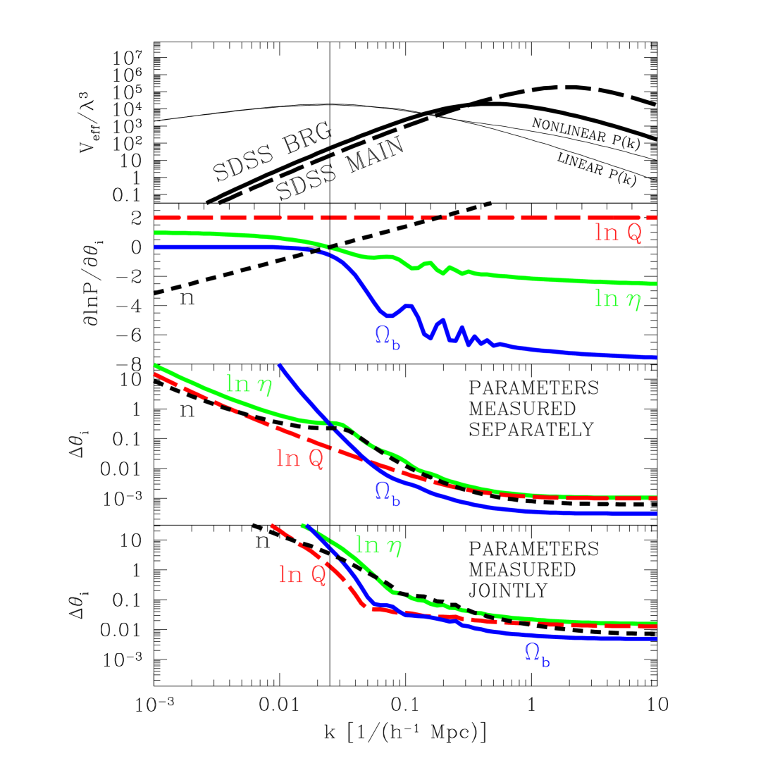
FIG. 1.: The top panel shows the weight functions $w(k)$ for main and BRG samples of the SDSS, together with our fiducial linear and nonlinear CDM power spectra in $(h^{-1}{\rm Mpc})^{3}$ units. The second panel shows the logarithmic derivatives of the linear power spectrum with respect to its amplitude, horizontal location, slope and baryon content. The third panel shows the accuracy with which these parameters can be measured using information on wavenumbers up to $k={k_{max}}$ when the other parameters are already known, and the bottom panel shows the corresponding accuracies when all four parameters must be determined simultaneously. The vertical line indicates $k_{*}$, the location where $P(k)$ peaks.

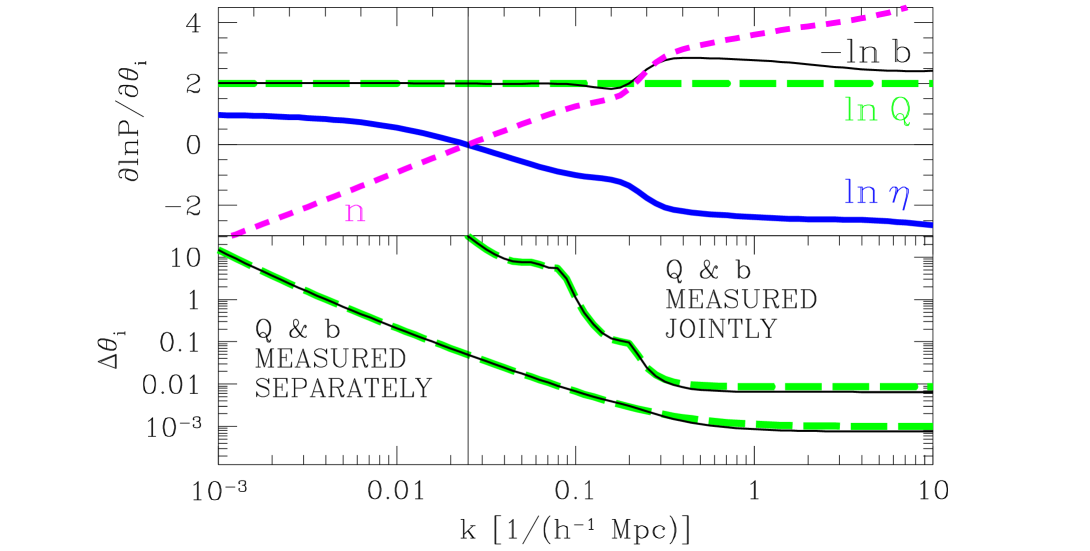
FIG. 2.: Similar to Figure 1, but using nonlinear power spectra. In the bottom plot, all parameters except $Q$ and $b$ are assumed to be independently known.

REFERENCES

- [1] G. Jungman, M. Kamionkowski, A. Kosowsky, and D. N. Spergel, Phys. Rev. Lett. 76, 1007 (1996).
- [2] G. Jungman, M. Kamionkowski, A. Kosowsky, and D. N. Spergel, Phys. Rev. D 54, 1332 (1996).
- [3] J. R. Bond, G. Efstathiou, and M. Tegmark, preprint astro-ph/9702100.
- [4] M. Zaldarriaga, D. Spergel, and U. Seljak 1997, preprint astro-ph/9702157.
- [5] Strauss, M. 1997, preprint astro-ph/9610033.
- [6] J. E. Gunn & D. H. Weinberg, in Wide-Field Spectroscopy and the Distant Universe, ed. S. J. Maddox and A. Aragón-Salamanca (World Scientific, Singapore, 1995).
- [7] M. Tegmark, A. N. Taylor, and A. F. Heavens, ApJ 480, 22 (1997).
- [8] M. G. Kendall & A. Stuart, The Advanced Theory of Statistics, Volume II (Griffin, London, 1969).
- [9] M. S. Vogeley & A. S. Szalay, ApJ 465, 43 (1996).
- [10] A. J. S. Hamilton 1997, preprints astro-ph/9701008 and astro-ph/9701008, MNRAS, in press.
- [11] H. A. Feldman, N. Kaiser, and J. A. Peacock, ApJ 426, 23 (1994).
- [12] M. Tegmark, Phys. Rev. D 55, 5895 (1997).
- [13] U. Seljak & M. Zaldarriaga, ApJ 469, 437 (1996).
- [14] J. R. Bond & G. Efstathiou, ApJ 285, L45 (1984).
- [15] W. Hu & N. Sugiyama, ApJ 471, 542 (1996).
- [16] D. Goldberg & M. Strauss 1997, preprint astro-ph/9707209.
- [17] B. Jain, H. J. Mo & S. D. M. White, MNRAS 276, L25 (1995).
- [18] D. H. Weinberg 1995, in “Wide-Field Spectroscopy and the Distant Universe”, eds. Maddox & Aragón-Salamanca (World Scientific, Singapore)