A New Approach to Probing Large Scale Power with Peculiar Velocities

Abstract

We propose a new strategy to probe the power spectrum on large scales using galaxy peculiar velocities. We explore the properties of surveys that cover only two small fields in opposing directions on the sky. Surveys of this type have several advantages over those that attempt to cover the entire sky; in particular, by concentrating galaxies in narrow cones these surveys are able to achieve the density needed to measure several moments of the velocity field with only a modest number of objects, even for surveys designed to probe scales $\mathrel{\raise 1.29167pt\hbox{$>$\kern-7.5pt\lower 4.30554pt\hbox{$\sim$}}}100$$h^{-1}$Mpc. We construct mock surveys with this geometry and analyze them in terms of the three moments to which they are most sensitive. We calculate window functions for these moments and construct a $\chi^{2}$ statistic which can be used to put constraints on the power spectrum. In order to explore the sensitivity of these surveys, we calculate the expectation values of the moments and their associated measurement noise as a function of the survey parameters such as density and depth and for several popular models of structure formation. In addition, we have studied how well these kind of surveys can distinguish between different power spectra and found that, for the same number of objects, cone surveys are as good or better than full-sky surveys in distinguishing between popular cosmological models. We find that a survey with $200-300$ galaxy peculiar velocities with distance errors of $15\%$ in two cones with opening angle of $\sim 10^{\circ}$ could put significant constraints on the power spectrum on scales of $100-300$$h^{-1}$Mpc, where few other constraints exist. We believe that surveys of the kind we describe her could provide a valuable tool for the study of large scale structure on these scales and present a viable alternative to full sky surveys.

Subject headings: cosmology: distance scales – cosmology: large scale structure of the universe – cosmology: observation – cosmology: theory – galaxies: kinematics and dynamics – galaxies: statistics

1 Introduction

One of the most important goals of cosmology is to determine the power spectrum of initial density fluctuations in the Universe. The primary tools in this endeavor have been redshift surveys, which have been used to probe scales $\mathrel{\raise 1.29167pt\hbox{$<$\kern-7.5pt\lower 4.30554pt\hbox{$\sim$}}}100$ $h^{-1}$Mpc, and microwave background anisotropy measurements, which tell us about the power spectrum on scales $\mathrel{\raise 1.29167pt\hbox{$>$\kern-7.5pt\lower 4.30554pt\hbox{$\sim$}}}1000$ $h^{-1}$Mpc (we use $h=H_{o}/(100$ km/s/Mpc) where $H_{o}$ is the Hubble constant). The gap between these scales, where we have relatively little knowledge of the power spectrum, is notable in several respects. First, theoretical considerations tell us that the power spectrum should have a maximum in this region at a scale corresponding to the horizon size at the time that the Universe became matter dominated. While redshift surveys have hinted that the power spectrum does indeed turn over at a scale $\sim 200$ $h^{-1}$Mpc (e.g. Fisher et al. 1993, Feldman et al. 1994), the errors inherent in the measurement are too large to be definitive. Further, several recent studies have suggested that there might be much more power on these scales than is usually assumed in models of large scale structure formation (Broadhurst et al.  1990, Landy et al.  1996, Ainasto et al.  1996.) If these suggestions are correct it will have important ramifications for our understanding of how structure formed in the Universe.

There are several observations planned or in progress that will attempt to study the power spectrum in this regime. From above, there are the small angle microwave anisotropy measurements. From below, the next generation redshift observations should significantly extend the range over which surveys can reliably determine the power spectrum. However, it may be a decade or longer before these ambitious and complex projects will produce measurements of the power spectrum on scales $\sim 200$ $h^{-1}$Mpc.

A third method of measuring the power spectrum on large scales involves the study of large scale motions of galaxies. There were several recent attempts to determine the power spectrum from observations of peculiar velocities. Kolatt & Dekel (1997) use the POTENT reconstruction of the density field to determine P(k). Zaroubi et al.  (1996) estimated the power spectrum from the Mark III catalog of peculiar velocities using Bayesian statistics. One advantage of this method is that the large scale velocity field probes the matter distribution in the Universe directly, and not merely the light distribution as redshift surveys do. However, the errors in velocity estimates are typically some fraction of the distance of the sample points, which in the case of distant objects can mean that the errors are larger than the peculiar velocity being measured. This is partially rectified by measuring only the lowest moment of the velocity field, namely the bulk flow. Since the bulk flow is, in a sense, an average of the velocities in the sample, its error is reduced over that of an individual measurement by the square root of the number of objects.

Two recent efforts to measure the bulk velocities of large volumes have resulted in contradictory conclusions. Lauer & Postman (LP 1994) found that the inertial frame defined by Abell clusters within $15,000$km/s exhibits a bulk velocity of $\approx 700$ km/s with respect to the cosmic microwave background (CMB) rest frame. More recently, Riess et al. (RPK 1995) used type Ia supernovae to measure the bulk velocity of a similar volume; their results are consistent with their sample being at rest relative to the CMB rest frame. In recent analyses (Feldman & Watkins 1994, Strauss et al. 1995, Jaffe & Kaiser 1995, Watkins & Feldman 1995) it was shown that both power spectra from structure formation models as well as results from redshift surveys are inconsistent with the LP measurement at the $2-3\sigma$ level, whereas they are quite consistent with the RPK result. Furthermore, the RPK and LP results seem to be inconsistent with each other at a high confidence level.

Abell clusters and type Ia supernovae are rare, thus the LP and RPK samples are by necessity quite sparse. This limits their ability to accurately measure moments of the velocity field beyond the bulk flow. In addition, obscuration by our Galaxy strongly constrains how accurately these surveys can ascertain components of the bulk flow in the plane of the Galaxy. Thus the only component of the bulk flow that LP and RPK are able to report with a reasonable significance is that along the Galactic poles. In this Letter we propose an alternative approach to gathering full sky surveys of peculiar velocities; we explore the possibility of probing the power spectrum on large scales by measuring the velocities of galaxies in only small patches of the sky. While this survey will necessarily be sensitive to only one component of the bulk flow, the increase in the density of objects will allow more accurate measurement of higher moments of the velocity field. An added advantage of this approach is that the higher moments probe a different range of scales than the bulk flow, making it possible to constrain the power spectrum more precisely.

We examine several factors necessary for the design of a useful peculiar velocity survey. We concentrate on surveys which cover two fields directly opposite to each other. These surveys can probe larger scales and are less susceptible to radial biases than one-sided surveys. We construct mock catalogs for these surveys and show how their sensitivity depends on depth and the number of objects measured. In particular, we calculate the expectation values and expected errors associated with the three most easily measured moments assuming several different power spectra.

2 Analysis

As stated above, individual velocity measurements are too noisy to allow us to accurately map the peculiar velocity field $\vec{v}(\vec{r})$. Instead we expand $\vec{v}(\vec{r})$ in a given region in terms of its moments (Kaiser 1991, Jaffe & Kaiser 1995),

$$v_{i}(\vec{r})=u_{i}+r_{j}p_{ij}+r_{j}r_{k}q_{ijk}+\dots$$ (1)

Here, $u_{i}$ and $p_{ij}$ are usually referred to as the bulk flow and the shear tensor respectively.

In practice we can measure only the radial component of velocities. Thus if our objects lie in a cone around a direction given by $\hat{R}$, we will be most sensitive to the component of the velocity along $\hat{R}$, $v_{R}=\vec{v}\cdot\hat{R}$. For this situation it is sufficient to model the velocity as being entirely along the $\hat{R}$ direction and depending only on $\vec{r}\cdot\hat{R}$, giving us a much simpler expansion,

$$v_{R}(\vec{r}\cdot\hat{R})=U_{1}+U_{2}(\vec{r}\cdot\hat{R}/R_{o})+U_{3}(\vec{r}\cdot\hat{R}/R_{o})^{2},$$ (2)

where we have introduced the arbitrary scale $R_{o}$ in order that the constants $U_{i}$ will all have the same units. In most of the analysis below we choose $R_{o}=100$$h^{-1}$Mpc. The constants $U_{i}$ represent the one component each of $u_{i}$, $p_{ij}$, and $q_{ijk}$ to which these surveys are most sensitive.

In terms of this model, the estimated line–of–sight velocity $S_{n}$ measured for the $n$th galaxy at a position $\vec{r}_{n}$ can be written as $S_{n}=\sum_{i=1}^{3}F_{n,i}\ U_{i}+\epsilon_{n}$, where $F_{n,i}=(\hat{r}_{n}\cdot\hat{R})(\vec{r}_{n}\cdot\hat{R}/R_{o})^{i-1}$. Here we assume that the noise $\epsilon_{n}$ is drawn from a Gaussian with zero mean and variance $\sigma_{n}^{2}+\sigma_{*}^{2}$, where $\sigma_{n}$ is the estimated uncertainty in the measurement of the line-of-sight velocity and $\sigma_{*}$ is introduced to account for contributions to the velocity of the galaxies in the survey arising from nonlinear effects as well as from the components of the velocity field that we have neglected in our model (Kaiser 1988). We shall take $\sigma_{*}=400$ km/s for all of our calculations, although in practice this choice makes little difference given the large values of $\sigma_{n}$ for most of the galaxies that we will consider.

Given a sample of objects with positions $\vec{r}_{n}$ and line-of-sight velocities $S_{n}$, the maximum likelihood solutions for the constants $U_{i}$ are given by

$$U_{i}=(A^{-1})_{ij}\sum_{n}{F_{n,j}\ S_{n}\over(\sigma_{n}^{2}+\sigma_{*}^{2})},$$ (3)

where the matrix $A_{ij}=\sum_{n}{F_{n,i}\ F_{n,j}\over(\sigma_{n}^{2}+\sigma_{*}^{2})}$; here and below we use the Einstein summation convention for repeated indices.

The theoretical expectations for the constants $U_{i}$ can be expressed in the form of a covariance matrix, $R_{ij}=\langle U_{i}U_{j}\rangle=R^{(v)}_{ij}+(A^{-1})_{ij}\$where $R^{(v)}_{ij}$ is the contribution from the velocity field and $(A^{-1})_{ij}$ is the noise. The matrix $R^{(v)}_{ij}$ is obtained by convolving the power spectrum with a window function,

$$R^{(v)}_{ij}={1\over(2\pi)^{3}}\int P_{(v)}(k)W^{2}_{ij}(k)\ d^{3}k={H^{2}f^{2}(\Omega_{o})\over 2\pi^{2}}\int P(k)W^{2}_{ij}(k)\ dk,$$ (4)

where we have used the fact that in linear theory there is a simple relationship between the velocity and density power spectrum, $P_{(v)}(k)=(H^{2}/k^{2})f^{2}(\Omega_{o})P(k)$, with $f(\Omega_{o})\approx\Omega^{0.6}$.

The tensor window function $W^{2}_{ij}(k)$ is calculated from the positions and velocity errors of the objects in the survey,

$$W^{2}_{ij}(k)={1\over 4\pi}\int d\theta\ d\phi\ {\rm sin}\theta\ W_{i}(k)W^{*}_{j}(k),$$ (5)

where

$$W_{i}(k)=(A^{-1})_{ij}\sum_{n}{{\hat{k}}\cdot{\hat{r}_{n}}\ F_{n,i}\ e^{i\vec{k}\cdot{\vec{r}_{n}}}\over(\sigma_{n}^{2}+\sigma_{*}^{2})}.$$ (6)

Once we have calculated $R_{ij}$ for a given power spectrum, we can construct a $\chi^{2}$ statistic $\chi^{2}=U_{i}\ R^{-1}_{ij}\ U_{j}$ for the three degrees of freedom of the measured moments. This statistic can be used to assess the compatibility of the power spectrum with the measured $U_{i}$. We note that the this statistic properly accounts for the correlations between the moments, which can be important for a sparsely sampled survey. Alternatively, given a parameterization of the power spectrum, $R_{ij}$ can be used in a likelihood analysis to determine the most likely values of the parameters (see, e.g. , Jaffe & Kaiser 1995).

In designing a survey, it is important to determine how well it can distinguish between different power spectra. We can quantify this by calculating the expectation value of the $\chi^{2}$ for power spectrum $P_{A}(k)$ given that the true power spectrum of the Universe is power spectrum $P_{B}(k)$:

$$\langle\chi^{2}_{AB}\rangle=\langle(U_{B})_{i}(R_{A}^{-1})_{ij}(U_{B})_{j}\rangle=(R_{A}^{-1})_{ij}\langle(U_{B})_{i}(U_{B})_{j}\rangle=(R_{A}^{-1})_{ij}(R_{B})_{ij}=Tr(R_{A}^{-1}R_{B}),$$ (7)

where subscripts denote quantities calculated assuming power spectra $P_{A}$ and $P_{B}$. The value of $\langle\chi^{2}_{AB}\rangle$ can be used to estimate the confidence level at which one can rule out power spectrum $P_{A}$ in a universe with power spectrum $P_{B}$ given a particular catalog of objects and assumed velocity errors.

We constructed mock catalogs of fixed number of galaxies restricted to two cones on opposite sides of the sky. We found that the results were roughly independent of the opening angle $\alpha$ of the cone as long as $\alpha<30^{\circ}$, giving some flexibility in the design of a survey. The results we report in this Letter are for $\alpha=10^{\circ}$. Galaxies were distributed radially using a selection function obtained by fitting an analytical function (cf. Feldman et al. 1994) to the radial distributions of various magnitude limited Tully-Fisher surveys (we used different surveys from the Mark III Catalog of Peculiar Velocities [Willick et al. , 1995, 1996]). We adjusted the depth of the survey by varying the location of the peak of the distribution function, $R_{o}$, which is directly related to the magnitude limit. For definiteness, we assumed the error in the measured velocity of a galaxy to be $15\%$ of its distance, an error commonly reported for Tully-Fisher distance measurements.

Given a mock survey, we can calculate the window functions for the three moments and determine which scales they are sensitive to. Assuming a power spectrum, we can also calculate the expected values of $U_{i}$ and their associated noise. It is useful to define the parameters

$$Q_{i}\equiv{R_{ii}^{(v)}\over(A^{-1})_{ii}},$$ (8)

that indicate how accurately a given survey can measure each of the three moments. Ideally we would like $Q_{i}\mathrel{\raise 1.29167pt\hbox{$>$\kern-7.5pt\lower 4.30554pt\hbox{$\sim$}}}1$ for each of the three moments. The geometry and density of the survey can be optimized to meet this requirement with the minimal observational effort. Although $U_{i}$ can in principle be correlated, we found that these correlations are small.

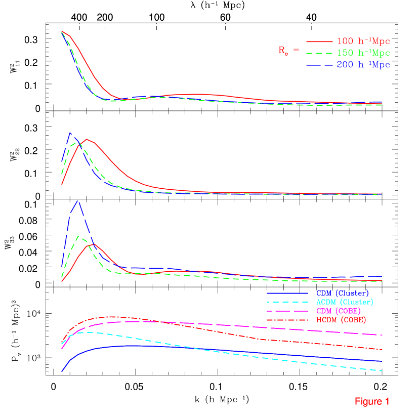
Figure 1: In the top three panels we plot the window functions associated with the moments $U_{1}$, $U_{2}$, and $U_{3}$ for different values of $R_{o}$, the location of the peak of the radial selection function for mock surveys of 200 galaxies. In the bottom panel we see the power spectra we used in our analysis. To find the expectation values of the different moments we integrate the product of the window functions of the top three panels with each of the power spectra.

In Figure 1 we see a series of normalized window functions from three mock surveys with different values of $R_{o}$, each with the same number of galaxies ($n=200$). While the window function for the bulk flow ($U_{1}$) has a maximum at $k=0$, the window functions for $U_{2}$ and $U_{3}$ are peaked at smaller scales. Thus we see that the higher moments probe a different region of the power spectrum than the bulk flow. Since we are looking only at a single component of the velocity along the direction of the survey, the angular distribution of the objects is relatively unimportant and edge effects are negligible.

In the bottom panel of Figure 1 we show the power spectra we used to calculate expectation values for the moments; standard COBE normalized CDM (Bardeen et al.  1986) and HCDM (Klypin et al.  1993) as well an $\Omega=1$ CDM normalized the observed abundance of clusters (see, e.g. Eke et al.  1996) and $\Lambda$CDM normalized to both cluster abundance and COBE.

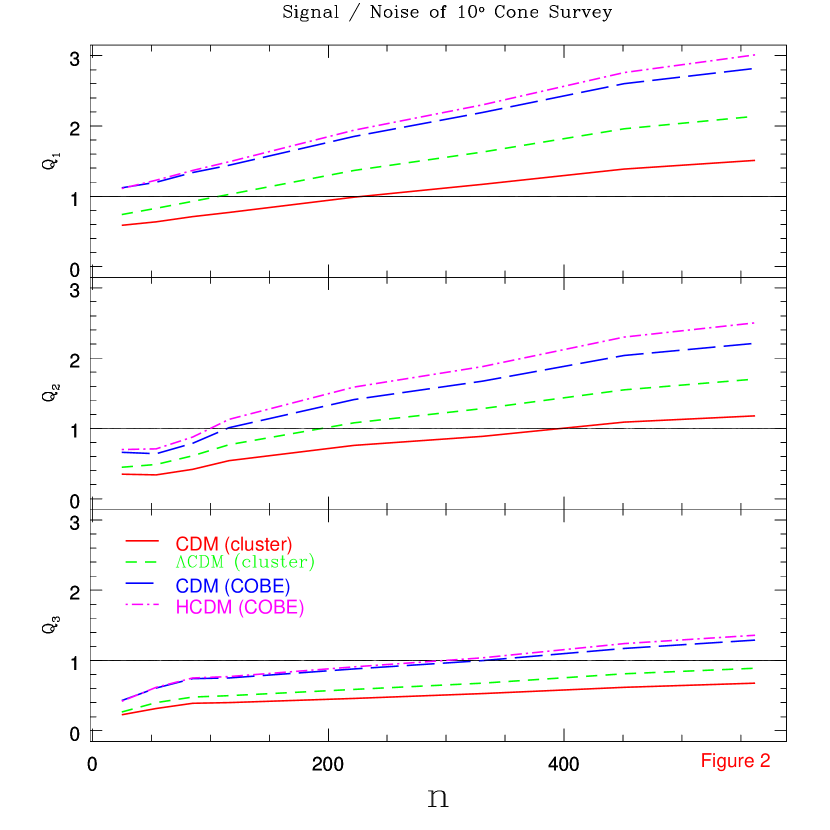
Figure 2: Here we see the values of $Q_{i}$ for different power spectra as a function of the number of objects in the survey. $Q_{i}$ rises with the number of points as expected as the noise inherent in the measurement becomes smaller with increased density.

In Figure 2 we show the $Q_{i}$ parameters (Eq. 8) for the three moments for a survey with $R_{o}=100$$h^{-1}$Mpc (effective depth $\approx 200$$h^{-1}$Mpc) using the four power spectra described above. We see that we need some $200-300$ galaxies in our survey to get $Q_{i}\sim 1$ for the power spectra we consider that produce the largest velocities, i.e. COBE normalized CDM and HCDM.

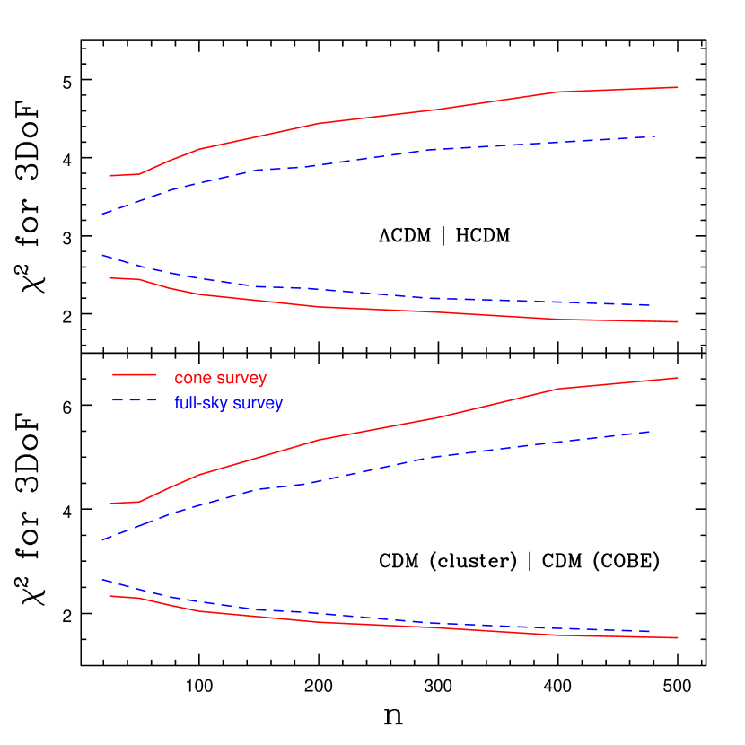
Figure 3: The $\chi^{2}$ for 3 degrees of freedom for HCDM normalized to COBE given a Universe with $\Lambda$CDM, and vice versa, for $10^{\circ}$ cone surveys, with the three lowest moments and for a full-sky survey (with the zone-of-avoidance removed) using the three bulk flow components as the three degrees of freedom, as a function of the number of objects. The full–sky surveys have the same radial distribution and errors as the cone surveys. We also show the $\chi^{2}$ for COBE normalized CDM and cluster normalized CDM. From the figure we see that the three moments calculated for the cone survey do better than the three bulk-flow components of the full-sky survey at distinguishing between the models for the same number of observed galaxies.

In the upper panel of Figure 3 we show the $\chi^{2}$ for three degrees of freedom for distinguishing between HCDM and $\Lambda$CDM in a $10^{\circ}$ cone survey with $R_{o}=100$$h^{-1}$Mpc as a function of the number of objects. The upper curve is for HCDM assuming that the true power spectrum is $\Lambda$CDM; here the $\chi^{2}>3$ since we are testing a model with excess power relative to the actual spectrum. The lower curve is for $\Lambda$CDM assuming the true spectrum is HCDM, which will give $\chi^{2}<3$. From these $\chi^{2}$ values, one can assign a confidence level at which the models are ruled out. In general, one can rule out spectra with excess power at a higher confidence level. For comparison, we show the same quantities for a full-sky survey (with the zone-of-avoidance removed) using the three bulk flow components as the three degrees of freedom; these surveys have the same radial distribution, number of objects and errors as the cone surveys. In the lower panel we show the $\chi^{2}$ for COBE normalized CDM given cluster normalized CDM and vice versa. From the figure we see that the three moments calculated for the cone survey do better than the three bulk-flow components of the full-sky survey at distinguishing between the models for the same number of observed galaxies.

A more complete comparison between full-sky and cone surveys would include information from higher moments of the full-sky survey. However, for the surveys and power spectra we have considered, the signal to noise of these higher moments is small. Results from analyses including the highest signal to noise moments suggest that cone surveys continue to be as good or better at distinguishing spectra.

3 Conclusions

In this Letter we have explored the properties of proper distance surveys that cover small fields in two opposing directions. Our analysis exploits the fact that a small area survey can measure some of the moments of the velocity field much more accurately than a full sky survey with the same number of objects. We have shown how to expand the velocity field in moments and constructed a $\chi^{2}$ test useful for constraining models. In order to get a “signal to noise” of unity for the three lowest moments, we found that a survey of $\approx 200-300$ galaxies is needed if we assume distance indicators accurate to about $15\%$ of the distance in a cone survey with opening angle of ${\cal O}(10^{\circ})$ and consider survey depths $\sim 200$$h^{-1}$Mpc. We have also shown that cone surveys are as good or better than full-sky surveys at distinguishing between cosmological models. These surveys could put important constraints on the power spectrum on large scales with only a modest observational effort, and thus could provide a valuable tool in probing scales that have been up to now largely beyond our scope.

Acknowlegements: We would like to thank Nick Kaiser for many conversations. We would also like to thank Michael Strauss, Gary Wegner and Jeff Willick for many thoughtful comments. HAF was supported in part by the NSF EPSCoR Grant and the University of Kansas GRF. RW was supported in part by NSF grant PHY-9453431 and NASA grant NAGW-4720.

References

- (1) Bardeen, J. M., Bond, J. R., Kaiser, N. & Szalay, A. S. 1986 ApJ 304 15
- (2) Broadhurst, T. J. Ellis, R. S. Koo, D. C. & Szalay, A. S. 1990 Nature 343 726
- (3) Einasto, J. et al. 1997 Nature385 139 - 141
- (4) Eke, V. R., Cole, S., & Frenk, C. S. 1996, MNRAS 282,263.
- (5) Feldman, H. A., Kaiser, N. & Peacock J. A. 1994 ApJ 426 23–37
- (6) Feldman, H. A. & Watkins, R. 1994 ApJ 430 L17–20
- (7) Jaffe, A. & Kaiser, N. 1995 ApJ 455 26
- (8) Kaiser, N. 1991 ApJ 366 28
- (9) Kaiser, N. 1988 MNRAS 231 149
- (10) Klypin, A., Holtzman, J., Primack, J. & Regős, E. 1993 ApJ 413 P48
- (11) Kolatt, T & Dekel, A 1997 ApJ 479 592
- (12) Landy et al. , 1996 ApJ 456 L1 (LCRS)
- (13) Lauer, T. & Postman, M. 1994 ApJ4̇25 418–38 (LP)
- (14) Riess, A. G., Press, W. H., & Kirshner, R. P. 1995, ApJ 438, L17 (RPK)
- (15) Strauss, M., Cen, R., Ostriker, J. P., Postman, M. & Lauer, T. 1995 ApJ 444 507
- (16) Watkins, R. & Feldman, H. A. 1995 ApJ 453 L73–76
- (17) Willick, J. et al. 1995 ApJ 446 12
- (18) Willick et al. 1996 ApJ 457 460
- (19) Zaroubi, S. et al. 1996 astro-ph/9610226