UV to X-ray Spectra of Radio-Quiet Quasars. Comparison With Accretion Disk Models

Abstract

We present UV to soft X-ray spectra of 31 radio-quiet quasars, comprising data from the IUE ULDA database and the ROSAT pointed observation phase. 90 % of the sample members show a soft X-ray excess above an underlying hard X-ray power law spectrum. Particularly for the steep X-ray spectrum ($\alpha_{\rm energy}>1.5$), low redshift subsample (17 objects) the X-ray spectral power law index is strongly correlated with the optical to X-ray broad-band spectral index $\alpha_{\rm ox}$, indicating that the main contribution to the soft X-ray and optical emission is due to the same emission component. We model the UV/soft X-ray spectra in terms of thermal emission from a geometrically thin $\alpha$-accretion disk. The structure and radiation field of the disk is calculated self-consistently and Compton scattering is treated by the Kompaneets equation. All relativistic effects on the disk structure and the emergent disk spectrum are included. Satisfactory spectral fits of the UV and soft X-ray continuum spectra are achieved when additional non-thermal hard X-ray and IR power law emission components are taken into account. The UV and soft X-ray spectra are well described by emission resulting from accretion rates in the range $\sim$ 0.1 to $\sim$ 0.3 times the Eddington accretion rate. Low mass/low redshift objects are found to accret at $<0.15\;\dot{M}_{\rm Eddington}$. Correlations of the accretion disk parameters with $\alpha_{\rm ox}$ are discussed.

1 Introduction

It is a well established fact that the maximum of the spectral energy distribution of quasars occures in the largely unobservable spectral range between the extrem UV and the soft X-ray domain. In many objects a steepening of the spectrum in the soft X-ray range as compared to the hard X-rays is observed which, in combination with the turnover of the spectrum in the UV range, suggests that these two components combine in the largely unobservable range between $\sim 3\times 10^{15}$ Hz and $\sim 3\times 10^{16}$ Hz to form the so called big blue bump emission. Continued attempts have been made to derive a self-consistent emission model which is able to account for this spectral component, the most probable scenario being thermal emission from an accretion disk around a central super-massive compact object.

The theory of standard geometrically thin $\alpha$-accretion disks is largely based on the paper of Shakura & Sunyaev ([1973]) and a general relativistic version presented by Novikov & Thorne ([1973]). It has soon turned out that simple accretion disk models based on multi-temperature blackbody emission from an optically thick accretion disk (Malkan & Sargent [1982], Malkan [1983]), at sub-Eddington accretion rates, are not sufficiently hot, or else that highly super-Eddington accretion rates would be required, for the accretion disk to emit an appreciable fraction of the radiation in the soft X-ray range (Bechtold [1987]). A number of authors have improved this simple model by considering various effects on the structure and emission spectrum of the disk. Czerny & Elvis ([1987]), and Wandel & Petrosian ([1988]) calculated the radiative transfer by including free-free opacities and the effects of Comptonization in a simple analytic manner. Bound-free opacities as well as relativistic effects were included by Laor & Netzer ([1989]) and Laor et al. ([1990]). Most computations of model spectra to date, however, adopted a given vertical structure or made use of an averaging in the vertical direction. A detailed investigation of the emission spectrum was performed by Ross, Fabian, & Mineshige ([1992]), using the Kompaneets equation (Kompaneets [1957]) to treat Compton scattering and including free-free and bound-free opacities of hydrogen and helium. They solved the vertical temperature structure and atomic level populations for a predetermined constant vertical density profile. A self-consistent solution of the vertical structure and radiative transfer is given by Shimura & Takahara ([1993]) and Shimura & Takahara ([1995]) for a Newtonian disk. In their viscosity description, they made the ad hoc assumption that the local heating rate is proportional to the mass density. In our approach (Dörrer et al. [1996]), the vertical structure and radiation field of a disk around a Kerr black hole is calculated in a self-consistent way. Moreover, we use a different viscosity description. In section 4 a short review of this model is given.

In the framework of the unified model the different properties of Active Galactic Nuclei are explained as being due to the different inclination angles under which the observer sees the accretion disk as well as various additional components such as absorbing material, emisssion line clouds or jets. The emission from the accretion disk is best studied in objects seen under intermediate inclination angles where the disk emission is neither obscured by an absorbing gas and dust torus nor is it swamped by beamed emission from a relativistic jet (in systems seen nearly face on). Such intermediate inclination angles are thought to lead to source properties as observed in radio-quiet quasars and Seyfert I galaxies. Thus, high signal-to-noise data, covering the spectral range from the UV to the soft X-ray range, of samples of such objects are best suited to investigate whether their broad-band spectra may be understood in terms of emission from an accretion disk. We have selected a sample of 31 radio-quiet quasars (see section 2 for a discussion of the selection criteria), which were observed both by IUE in the energy range from 130 to 305 nm and by ROSAT in the energy range from 0.1 keV ($\sim$ 3 nm) to 2.4 keV ($\sim$ 0.5 nm) in order to investigate whether the UV and soft X-ray spectra of these objects are in agreement with predictions based on our accretion disk emission model.

The X-ray emission in the ROSAT energy band consists of at least two components, a hard power law component, extending to higher X-ray energies, beyond the ROSAT energy range, and a soft component, known under the name of soft X-ray excess emission, which in many AGN dominates the spectrum at energies below $\sim$ 0.5 keV and which is widely thought to originate in the inner part of an accretion disk. Testing the predictions of our accretion disk model thus requires to separate the contributions of these two emission components. Due to the limited energy resolution of ROSAT and also due to its limited spectral coverage at higher X-ray energies ($<$ 2.4 keV), except for the brightest objects, this is not possible based on the ROSAT data alone. We therefore make use of published hard X-ray spectral slopes to separate the two emission components in our spectral fits. As a first approach we have compared spectra from deep ROSAT pointings with the hard power law spectra taken from the literature, to convince ourselves that soft excess emission is indeed present in almost all of the objects (see section 3).

Things are further complicated by the fact that in the UV range different spectral components contribute to the emission. We treat this by including an additional power law component in our model fits extending from the IR with an exponential cutoff at around $2\times 10^{15}$ Hz. Details on the model fitting performed and on the resulting distributions of the four accretion disk model parameters central mass $M$, mass accretion rate $\dot{M}$, viscosity parameter $\alpha$, and the inclination angle $\Theta$ can be found in section 5. A similar study using data from the ROSAT All Sky Survey based on an earlier version of the present accretion disk model is presented by Friedrich et al. (1997). A brief comparison of the two models and a summary of basic results is given in Staubert et al. (1997).

Table 1: The AGN Sample
ROR: ROSAT sequence number (PSPC). T is the exposure time in ks, z is the redshift of the object, and R the radio flux in mJy. The UV flux of IUE (LWP and SWP camera) is given in Jy. CR is the ROSAT PSPC count rate [cts/s] in the energy range 0.1 to 2.4 keV. See section 2 for details on the broad-band spectral indices $\alpha_{\rm ox}$.

	AGN	RA	DEC	ROR	T	z	R	mv	UV-flux		CR	$\alpha_{\rm ox}$
#	name	(2000)	(2000)						LW	SW
1	PG 0026$+$12	00 29 08	13 16 50	WG701456	2.73	0.142	2	15.4	1.02	1.08	0.413	1.381
2	PG 0052$+$251	00 54 47	25 26 19	WG701038	6.77	0.155	1	15.4	1.55	1.41	0.600	1.361
3	TON S210	01 21 43	-28 20 01	US700445	4.53	0.117	-	14.9	-	1.72	2.000	1.410
4	MARK 1014	01 59 44	00 24 08	WG700225	6.25	0.163	8	15.7	-	0.99	0.209	1.607
5	NAB 0205$+$02	02 07 43	02 43 21	US700432	14.07	0.155	2	15.4	1.60	0.91	0.667	1.523
6	PG 0804$+$761	08 10 59	76 02 14	WG700470	3.77	0.100	2	15.1	3.60	2.60	1.194	1.316
7	IRAS 09149$-$6206	09 16 00	-62 20 11	WG701484	1.89	0.057	16	13.6	3.22	0.96	0.405	1.741
8	HE 1029$-$1401	10 31 48	-14 17 51	WG700461	13.59	0.086	-	13.9	6.18	3.80	1.830	1.432
9	PG 1049$-$005	10 51 45	-00 52 20	US700381	4.74	0.357	-	16.0	0.88	0.37	0.044	1.677
10	Q 1101$-$264	11 03 19	-26 46 10	WG900525	5.12	2.148	-	16.0	2.41	-	0.036	1.589
11	PG 1116$+$215	11 19 02	21 18 13	WG700228	24.59	0.177	3	15.1	3.36	3.17	0.994	1.491
12	GQ COM	12 04 34	27 53 15	WG700232	14.42	0.165	1	15.6	-	0.90	0.400	1.432
13	PG 1216$+$069	12 19 15	06 37 45	US700021	3.46	0.334	4	15.7	-	0.86	0.395	1.427
14	PG 1247$+$268	12 49 59	26 30 13	WG701173	2.19	2.041	1	15.7	0.49	-	0.104	1.554
15	B 201	12 59 43	34 22 35	WG600164	17.17	1.375	13	16.9	0.34	-	0.049	1.487
16	PG 1307$+$085	13 09 41	08 19 15	WG700229	7.69	0.155	-	15.3	-	1.37	0.524	1.503
17	PG 1309$+$355	13 12 11	35 14 29	WG701079	6.24	0.184	43	15.5	-	0.59	0.260	1.686
18	IRAS 13349$+$2438	13 37 10	24 22 19	UK700553	3.32	0.107	7	15.0	0.70	-	0.954	1.584
19	PG 1352$+$183	13 54 27	18 04 44	US700804	5.63	0.152	-	15.7	0.97	0.74	0.403	1.481
20	PG 1407$+$265	14 09 15	26 17 36	US700359	3.23	0.947	8	15.8	1.01	0.51	1.074	1.251
21	PG 1415$+$451	14 16 52	44 55 18	US700805	7.43	0.114	-	15.7	-	0.44	0.335	1.657
22	PG 1416$-$129	14 18 58	-13 11 09	WG700527	9.11	0.129	4	15.4	0.61	0.34	0.378	1.389
23	PG 1444$+$407	14 46 37	40 34 23	US701371	5.62	0.267	-	15.8	-	0.74	0.334	1.640
24	PG 1522$+$101	15 24 16	09 58 09	US701001	10.02	1.325	-	16.0	0.96	0.44	0.026	1.775
25	PG 1543$+$489	15 45 20	48 45 37	US700808	7.18	0.400	1	16.3	0.64	-	0.115	1.685
26	MARK 876	16 13 44	65 42 47	WG700230	6.72	0.129	2	15.4	1.66	1.32	0.915	1.354
27	MARK 877	16 20 03	17 24 14	UK700274	9.57	0.114	1	15.4	1.65	-	0.117	1.578
28	PG 1630$+$377	16 31 52	37 37 30	WG700255	8.93	1.478	-	16.0	0.93	0.23	0.073	1.604
29	HS 1700$+$6416	17 00 47	64 11 57	WG701457	27.41	2.722	-	16.1	0.16	-	0.012	1.775
30	KUV 18217$+$6419	18 21 44	64 20 44	US700948	1.98	0.297	13	14.2	3.76	2.40	1.358	1.416
31	MR 2251$-$178	22 53 59	-17 33 50	UK701630	18.32	0.068	3	14.4	3.17	1.94	3.046	1.272

2 Sample selection and data analysis

We have selected a sample of bright radio-quiet objects from the Veron-Cetty & Veron ([1993]) and the Hewitt & Burbidge ([1993]) quasar catalogues by requiring the radio (flux measured at 5 GHz) to optical (V band) broad-band spectral index $\alpha_{\rm ro}$ to be flatter than 0.3 . For objects where no radio flux measurement was available, an upper limit of 25 mJy was assumed. Note that, through this selection criterium, objects weaker than $16.8^{\rm th}$ magnitude in the v band are only included in the sample when radio flux measurements are available and the radio flux is below 25 mJy, essentially resulting in a cutoff of the sample at $m_{\rm v}=16.8$ . All objects show broad emission lines and have absolute optical magnitudes brighter than M${}_{\rm v}=-23.5$ and are thus classified as quasars.

These objects were cross-correlated both with the list of ROSAT PSPC pointings from the ROSAT archive and with the IUE ULDA database of low resolution spectra. Objects were included in the sample when (1) at the time of the analysis (summer 1995), UV spectra were available in the ULDA database and the ROSAT data had entered the public domain, (2) the objects were located within 44 minutes of arc from the optical axis of the ROSAT observation, (3) they were not hidden by the PSPC support structure, (4) at least 180 PSPC source counts had been measured. The final sample defined in this way which was investigated in our further analysis consists of 31 objects, listed in Tab. 1.

Depending on the distance of the object from the optical axis of the ROSAT PSPC detector, X-ray counts were extracted within a circular area centered on the source position with radii ranging from 1 to 5 minutes of arc. For each object, the background was accumulated from an annulus centered on the source position from which areas contaminated by other sources had been excluded. The data were binned into background subtracted count rate spectra with, depending on the number of source counts, 6 to 23 spectral bins in the energy range from 0.1 to 2.4 keV (channel 11 to 240) and a dead time correction and a correction for telescope vignetting was applied. The binning was performed such that a S/N of at least 5 was achieved in each bin.

The broad-band spectral indices $\alpha_{\rm ro}$ and $\alpha_{\rm ox}$ used for the sample selection and in our statistical analysis were calculated from the source frame luminosity densities at 5 GHz, 2500 Å, and 2 keV, respectively, which were determined following Zamorani et al. ([1981]) and Marshall et al. ([1983]), and applying corrections for reddening following Seaton ([1979]). The resulting $\alpha_{\rm ox}$ values are listed in Table 1.

Data from the IUE ULDA database were used to determine continuum flux values in each of the frequency bands 130–140, 140–155, 166–170, and 170–185 nm (SWP camera) and 245–260, 260–275, 275–290, and 290–305 nm (LWP/LWR camera). The continuum flux level was determined by removing emission and absorption lines using a sliding window technique with window widths of 0.4, 0.8, 1.6, 3.2, 6.4, and 12.8 nm. De-reddening of the resulting continuum fluxes was performed by using ${\rm<N_{H}/E_{B-V}>=4.8\times 10^{21}\;cm^{-2}\;mag^{-1}}$ (Bohlin et al. [1987]) with galactic ${\rm N_{H}}$ values as derived from 21 cm radio measurements (Stark et al. [1992] and Elvis et al. [1989]).

Figure 1: Histograms of ROSAT best-fit spectral power law indices. The canonical hard X-ray spectral power law index, $\alpha=0.7$, as well as the mean hard X-ray spectral power law index, $\alpha=0.86$, of the sample members where measurements were available are marked by vertical lines. Lower panels: Histograms of change in spectral slope between ROSAT and hard X-ray band.

Figure 2: ROSAT spectral power law index plotted over redshift (left: linear scale; right: logarithmic scale). Each object is shown twice. Diamonds: Fits with free ${\rm N_{H}}$. Triangles: Fits with fixed ${\rm N_{H}}$. Open symbols refer to spectral fits where the $1\sigma$ statistical errors were larger than 0.3.

Table 2: ${\rm N_{H}}$ in units of $10^{20}{\rm cm}^{-2}$. The first ${\rm N_{H}}$ value (${\rm N_{H}}$ - fix) is taken from Elvis et al. [1989] if marked with a ^⋆, else from Stark et al. [1992]. $\alpha$ is the ROSAT spectral power law index, $\sigma_{\alpha}$ the corresponding $1\sigma$ error. $\sigma_{\rm N_{H}}$ ist the $1\sigma$ error of the fittet ${\rm N_{H}}$ value.

	${\rm N_{H}}$ - fix				${\rm N_{H}}$ - free
#	${\rm N_{H}}$		$\alpha$	$\sigma_{\alpha}$	${\rm N_{H}}$	$\sigma_{\rm N_{H}}$	$\alpha$	$\sigma_{\alpha}$
1	4.	93⋆	1.214	0.085	5.33	1.04	1.312	0.269
2	4.	50⋆	1.481	0.040	3.93	0.44	1.317	0.139
3	1.	67	1.771	0.026	1.61	0.19	1.746	0.093
4	2.	45	1.736	0.067	2.54	0.69	1.771	0.280
5	2.	99⋆	2.104	0.025	3.44	0.30	2.277	0.118
6	3.	12⋆	1.435	0.033	3.62	0.40	1.600	0.140
7	17.	96	1.351	0.270	7.15	2.45	0.610	0.386
8	6.	64	1.665	0.020	5.82	0.21	1.470	0.056
9	3.	97	1.798	0.330	0.98	1.07	0.687	0.769
10	5.	25	0.844	0.269	6.24	6.37	1.011	0.739
11	1.	44⋆	1.711	0.016	1.48	0.11	1.730	0.054
12	1.	72⋆	1.210	0.030	1.86	0.29	1.263	0.117
13	1.	47	1.298	0.059	1.92	0.55	1.488	0.238
14	1.	57	1.458	0.173	0.52	0.81	0.988	0.571
15	1.	90	1.605	0.115	1.01	0.85	1.213	0.422
16	2.	20⋆	1.627	0.037	2.18	0.36	1.617	0.153
17	1.	84	1.957	0.073	0.55	0.32	1.309	0.197
18	1.	09	1.808	0.049	1.09	0.28	1.812	0.162
19	1.	84⋆	1.526	0.051	1.43	0.39	1.352	0.182
20	1.	38⋆	1.602	0.040	1.52	0.32	1.665	0.153
21	1.	26	1.903	0.061	0.59	0.24	1.532	0.157
22	7.	20⋆	1.198	0.066	7.37	0.80	1.227	0.155
23	1.	11	1.943	0.066	1.08	0.37	1.928	0.207
24	3.	02	2.008	0.264	1.21	1.10	1.305	0.799
25	1.	59	1.949	0.101	2.38	0.88	2.315	0.416
26	2.	66⋆	1.499	0.029	2.59	0.31	1.473	0.120
27	4.	35⋆	1.128	0.110	3.43	1.08	0.877	0.328
28	0.	90⋆	1.446	0.113	1.64	0.87	1.835	0.463
29	2.	49	0.949	0.179	1.58	1.74	0.669	0.602
30	4.	15	1.522	0.054	1.84	0.51	0.800	0.182
31	2.	84⋆	1.331	0.010	2.36	0.10	1.160	0.037

Figure 3: Broad band power law index $\alpha_{\rm ox}$ plotted against ROSAT spectral power law index (fixed ${\rm N_{H}}$). Diamonds: redshift, $z<0.5$; triangles: $z>0.5$; open symbols: absorbed spectra (${\rm N_{H}}>3\cdot 10^{20}\;{\rm cm}^{-2}$). $1\sigma$ errors of the slope of the linear regression line calculated for the 17 steep X-ray spectrum objects ($\alpha_{\rm ROSAT}>1.5$) are marked as solid lines.

3 Spectral power law fits to the ROSAT data

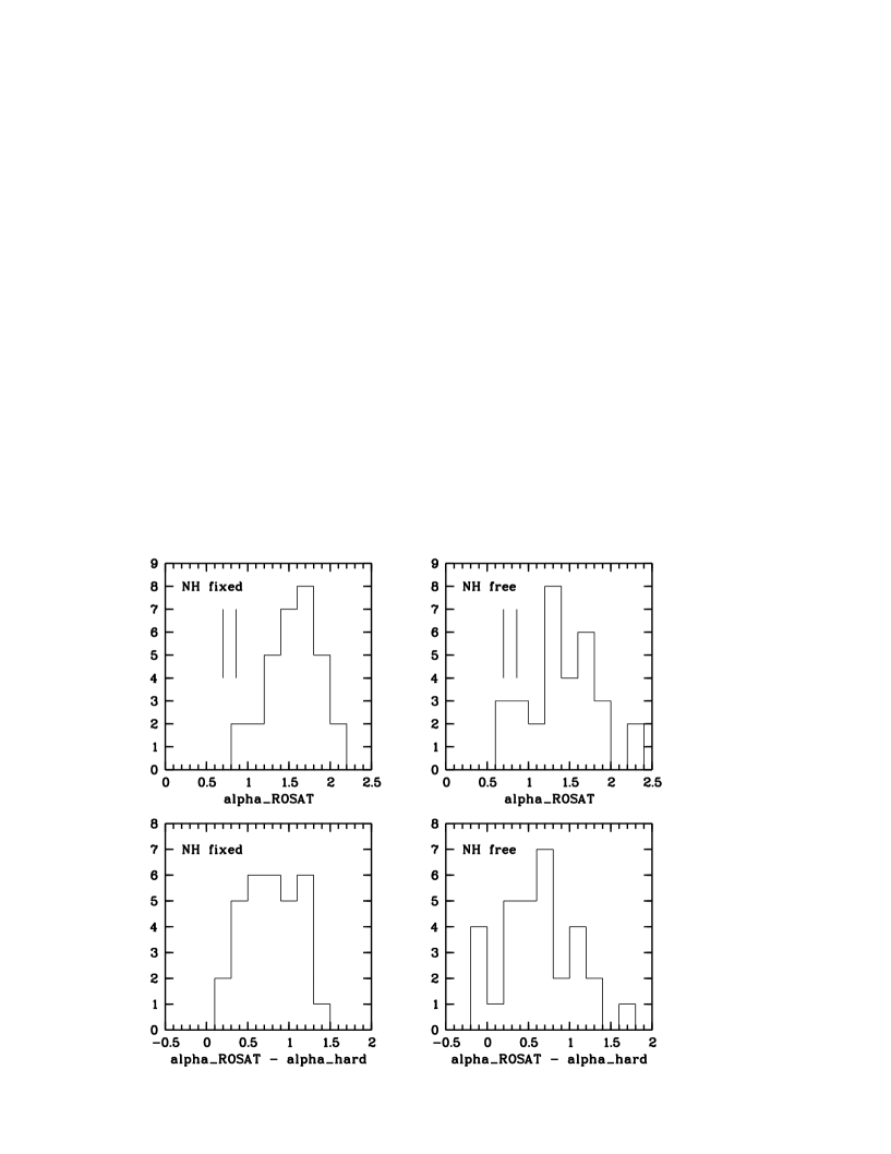
As a first approach to quantify the soft X-ray excess emission in the ROSAT energy window we have fitted power law spectra to the ROSAT count rates for all sample members. The distribution of the resulting spectral indices $\alpha_{\rm ROSAT}$ for a column density fixed at the galactic value and a free absorbing column density ${\rm N_{H}}$ are given in Fig. 1 (upper panels). For comparison, the canonical value, $\alpha_{\rm hard}=0.7$, and the sample mean, $<\alpha_{\rm hard}>$ = 0.86, of the hard X-ray power law are indicated as vertical lines. Except for a somewhat larger width of the distribution no large difference between the fixed, galactic ${\rm N_{H}}$ and free ${\rm N_{H}}$ power law spectral indices is observed, thus indicating that, on average, the spectra are not much affected by intrinsic low energy absorption in excess of the galactic value in the ROSAT spectral range. The spectral indices, together with the corresponding column densities ${\rm N_{H}}$, are summarized in Table 2. The mean ROSAT spectral power law indices for free and fixed ${\rm N_{H}}$ are 1.40 and 1.55, respectively, signifying a marked steepening of the spectrum as compared to the spectral slopes observed at higher energies. Looking at each object individually, a steepening of the spectral slope between the hard and soft X-ray range is found in almost all sample members. The mean change in spectral index is found to be 0.62 (free ${\rm N_{H}}$) and 0.78 (fixed ${\rm N_{H}}$), respectively. In Fig. 1 (lower panels) the distribution of this change in spectral index is shown.

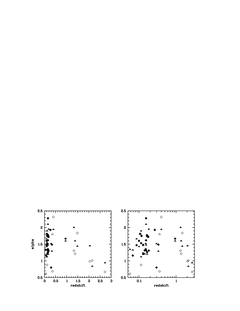
When going to objects at higher redshifts, the ROSAT sensitivity window is shifted to higher source frame energies, thus in effect turning ROSAT into a higher energy X-ray instrument. We find that at these higher source frame X-ray energies ROSAT does indeed measure harder X-ray spectral indices, similar to those of low redshift objects measured by higher energy X-ray instruments (see Fig. 2), in agreement with results by Schartel et al. (1996) and others. Note, however, that Puchnarewicz et al. ([1996]) do not find a dependence of the mean X-ray power law index on redshift in their sample of AGN from the RIXOS survey which may in part be due to the selection of their objects in the hard 0.4 – 2.0 keV ROSAT energy band.

Contrary to previous results, here, the dependence of the X-ray spectral index on redshift is visible in individual, relatively bright objects as opposed to averaged properties derived from stacked spectra or mean spectral indices of many weak objects. Based on radio flux measurements and upper limits all objects in the sample are known to be radio-quiet ($\alpha_{ro}<0.3$; see section 2). We can therefore exclude any contamination of our sample from high-redshift, radio-loud objects which are known to be more luminous than radio-quite quasars and at the same time display harder X-ray spectra. Such a contamination has previously been suggested as a possible cause of the observed dependence of the ROSAT power law indices on redshift. For the 7 objects in the redshift range $0.5<z<3.0$ a Spearman rank correlation coefficient of $-0.82\;(-0.75)$ is found, corresponding to a likelihood of 0.02 (0.05) for randomness of the $\alpha_{\rm ROSAT}-z$ correlation. Results for fixed ${\rm N_{H}}$ and free ${\rm N_{H}}$ (in brackets) spectral power law fits are given. A quantitativ analysis of this behaviour, using the accretion disk model described in the following section is presented in a forthcoming paper (Brunner et al., 1997). Note that the low redshift objects ($z<0.5$) in our sample do not follow this trend, suggesting a turnover of the $\alpha_{\rm ROSAT}-z$ relation in the redshift range $0.2<z<0.5$ with decreasing spectral indices on either side of this range. One possible interpretation for the turnover of the $\alpha_{\rm ROSAT}-z$ relation is that, as one goes to lower and lower redshifts, lower luminosity objects are detected where the accretion disk component is increasingly absorbed and the spectrum is increasingly dominated by the hard power law component. We would finally like to point out that the observed hardening of the ROSAT spectral indices with redshift rules out the possiblity that the steep AGN spectra observed by ROSAT may, as has been suggested, in part be due to errors in the cross-calibration of the ROSAT PSPC detector and previous higher energy X-ray instruments.

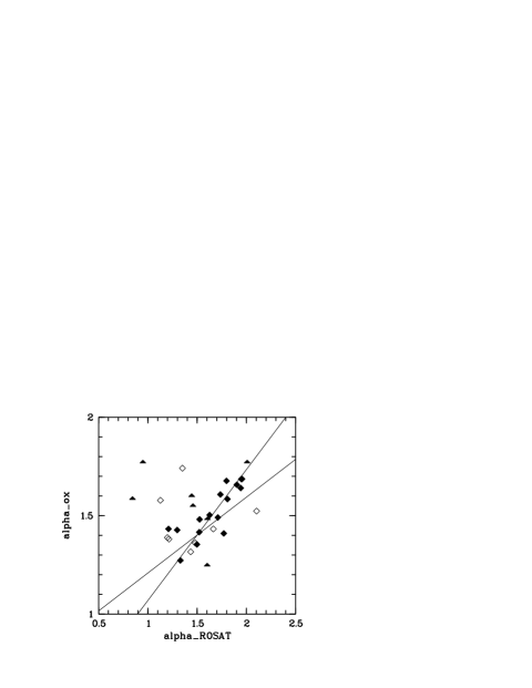
For the steep X-ray spectrum ($\alpha_{\rm ROSAT}\;{\rm(fixedN_{H})}>1.5$) subsample (17 objects) a strong correlation of the ROSAT spectral index (fixed ${\rm N_{H}}$) and the optical to X-ray broad-band spectral index is found (see Fig. 3). The correlation index is 0.78 (Spearman rank correlation coefficient), corresponding to a probability of $2.1\cdot 10^{-4}$ of randomness. This suggests that in objects with strong soft X-ray excess emission, i.e., objects with steep ROSAT spectra, the dominant contributions to the X-ray and UV/optical emission are due to the same physical emission component (i.e., the big blue bump emission). While the correlation can also be traced to objects with lower ROSAT spectral indices, a number of these objects show broad-band spectral indices which are considerably steeper than predicted by the correlation, suggesting that in these objects, the onset of the big blue bump emission is at or below the lower cutoff of the ROSAT sensitivity window. Note that a fraction of these objects (marked by filled triangles in Fig. 3) are at higher redshifts ($z>0.5$) where any blue bump emission component is expected to be shifted out of the ROSAT sensitivity window. Objects marked as open diamonds in Fig. 3 which also do not seem to follow the correlation are seen through absorbing column densities $>3\cdot 10^{20}$ cm^-2 and may thus be affected by uncertainties in the ROSAT power law index (fixed ${\rm N_{H}}$) and possibly the de-reddening of the optical fluxes. Similar correlations of $\alpha_{\rm ox}$ and $\alpha_{\rm x}$ have also been reported by Puchnarewicz et al. 1996.

While the change in spectral slope between the ROSAT and harder X-ray energy bands as well as the $\alpha_{\rm ROSAT}-\alpha_{\rm ox}$ correlation are useful indicators for the soft X-ray excess and big blue bump emission, a quantitative analysis is best performed in the framework of a physical emission model, the most widely advocated candidate being emission from the hot inner region of an accretion disk around a super-massive central object.

4 Accretion disk model used in spectral fits

We assume a standard geometrically thin $\alpha$-accretion disk around a massive Kerr black hole. A detailed description of our model is given in Dörrer et al. ([1996]). Here, we just summarize the basic concepts of the calculations. Model parameters are the mass $M$ of the central black hole, the accretion rate $\dot{M}$, the viscosity parameter $\alpha$, and the specific angular momentum $a$ of the central black hole. In addition to the parameters describing the physical properties of the accretion disks the inclination angle under which the observer sees the disk is also a free parameter. The specific angular momentum $a$ of the central black hole was fixed at $a=0$ in our spectral fits. All relativistic corrections on the disk structure with respect to a Newtonian model are included according to Riffert & Herold ([1995]).

The radiative transfer is solved in the Eddington approximation, and the plasma is assumed to be in a state of local thermodynamic equilibrium. Multiple Compton scattering is treated in the Fokker-Planck approximation using the Kompaneets operator. The absorption cross section contains only free-free processes for a pure hydrogen atmosphere. Induced contributions to the radiative processes have been neglected throughout.

For a given radial distance $R$ from the central black hole, a self-consistent solution of the vertical structure and radiation field of the disk is obtained from the hydrostatic equilibrium equation, radiative transfer equation, energy balance equation, and equation of state, when proper boundary conditions are imposed. Note, that we have not considered convection in our model.

In our calculations the viscosity is assumed to be entirely due to turbulence. Because the standard $\alpha$-description (viscosity proportional to the total pressure) leads to diverging temperature profiles in the upper parts of the disk, we have included the radiative energy loss of the turbulent elements in the optically thin regime. For the turbulent viscosity we then have

$$\eta=\alpha\;\rho\;H\;V_{\rm turb}~{},$$ (1)

where $\eta$ is the shear viscosity, $\rho$ is the mass density, $H$ is the self-consistently calculated height of the disk, $V_{\rm turb}$ is the upper limit for the velocity of the largest turbulent elements (see Dörrer et al. [1996] for details on the determination of $V_{\rm turb}$) and $\alpha$ is the viscosity parameter of our model.

We used a finite difference scheme in the vertical direction $z$ and in frequency space $\nu$ to find solutions of the given set of equations. The vertical structure was resolved with 100 points on a logarithmic grid, and 64 grid points were used in frequency space. The resulting set of algebraic difference equations was then solved by a Newton-Raphson method.

To get the overall structure and emission spectrum of the disk we calculated the vertical structure and the local emission spectrum at $50$ logarithmically spaced radial grid points from the last stable orbit to the outer disk radius (here $R_{\rm out}=1000\;R_{\rm S}$, where $R_{\rm S}=2GM/c^{2}$ is the Schwarzschild radius, $G$ is the gravitational constant, and $c$ is the velocity of light). The whole disk spectrum as seen by a distant observer at an inclination angle $\Theta_{0}$ with respect to the disk axis ($\Theta_{0}=0$ for a face-on observer) is then calculated by integration of the local spectra over the disk surface. All general relativistic effects on the propagation of photons from the disk surface to the observer are included, using a program code (Speith et al. 1995) to obtain values of the Cunningham transfer function (Cunningham [1975]) for any set of parameters.

The accretion disk spectrum as determined from the above calculations extends from the optical to the soft X-ray range ($<$ 1 keV), the maximum of the emission being in the far UV. Qualitatively, the dependence of the spectral shape on the model parameters is such that, if the mass accretion rate $\dot{M}$ is kept at a constant fraction of the Eddington accretion rate $\dot{M}_{\rm Eddington}$, the central mass $M$ mainly determines the total flux while approximately maintainig the spectral shape. Increasing the mass accretion rate in terms of the Eddington accretion rate $\dot{M}/\dot{M}_{\rm Eddington}$, on the other hand, while also increasing the total flux, makes the spectrum harder, i.e. a larger fraction of the flux is emitted in the X-ray range. Similarly, an increase of the viscosity parameter $\alpha$ also leads to a hardening of the spectrum. Going from low (disk seen face on) to high (disk seen edge on) inclination angles of the accretion disk, the total flux from the disk is reduced and at the same time a hardening of the spectrum due to Doppler boosting resulting from the rotation of the disk occures.

5 Model fits to the IUE and ROSAT data

We have performed $\chi^{2}$ fits to the UV to soft X-ray continuum spectra of the 31 sample quasars in order to investigate whether the observed spectra are indeed in agreement with our model, i.e. whether satisfactory best-fit minimum $\chi^{2}$ values are achieved and the resulting accretion disk model parameters are in line with our general understanding of the quasar phenomenon.

Figure 4: UV to X-ray spectra of sample members #15, #17, and #18, showing UV and ROSAT data points (crosses represent 1 $\sigma$ error bars) and model prediction (solid line). The accretion disk component (dot-dashed) and hard X-ray (long dashes) and IR (short dashes) power laws are displayed separately. The spectrum is plotted in the source frame. Residuals are given in units of $1\sigma$.

Figure 5: Distribution of best-fit accretion rates $\dot{M}$ in units of the Eddington accretion rate $\dot{M}_{\rm Eddington}$. Confidence contours (68 %, 90 %, 99 %) of the mean and width (Gaussian $\sigma$) of the distribution are plotted.

Figure 6: Distribution of best-fit viscosity parameters $\alpha$. Confidence contours (68 %, 90 %, 99 %) of the mean and width (Gaussian $\sigma$) of the distribution are plotted.

As already mentioned in the introduction, in order to separate the accretion disk emission from the underlying hard power law spectrum, where available we took the spectral index for the hard power law from the literature (Einstein Observatory, EXOSAT, GINGA; Malaguti et al., 1994). Otherwise, a canonical value of $0.7$ was adopted. X-ray variability between the observation in the soft and hard X-ray bands was allowed for by treating the normalization of the hard power law spectrum as a free parameter. The spectral indices and references used are listed in Table 4.

We have not included infrared and optical data in the spectral analysis, because such measurements were not available for all of the sample members and many different emission components (non-thermal synchrotron emission, thermal dust emission, BLR and NLR line emission, emission from the host galaxy) would needlessly complicate the analysis. Emission components at low frequencies which in addition to the accretion disk also contribute to the emission in the UV range were incorporated into the model by assuming a power law component with spectral index $\alpha=1.2$ and an exponential cutoff in the extreme UV range ($\nu=10^{16}$ Hz) which mainly represents the non-thermal synchrotron component.

Interstellar low energy X-ray absorption is included in our spectral fits by using the galactic hydrogen column densities by Stark et al. [1992] and Elvis et al. [1989] and by applying the cross sections by Morrison & Mc Cammon ([1983]). Note that the de-reddening of the UV data, based on the same hydrogen column densities, was already applied to the data prior to the spectral fitting (see section 2). We did not consider intrinsic absorption in the accretion disk model fitting. This is justified as no evidence for intrinsic absorption was found in our spectral power law fits and, generally, high luminosity objects (i.e. quasars as opposed to lower luminosity AGN) at moderate redshifts are not expected to show large amounts of intrinsic absorption.

The total fit function thus includes three components with a total of six free parameters:

1. Accretion disk model with four free parameters ($M$,$\dot{M}$,$\alpha$, $\Theta_{0}$)

2. Underlying hard power law with a slope taken from the literature (free normalization)

3. Soft power law with $\alpha=1.2$ and a cutoff in the EUV (free normalization).

The accretion rate $\dot{M}$ is measured in units of the Eddington accretion rate $\dot{M}_{\rm Edd}=L_{\rm Edd}/(\eta c^{2})$, where $L_{\rm Edd}=4\pi cGM/\kappa_{T}$ is the Eddington luminosity, $\eta$ is the efficiency of accretion, and $\kappa_{T}$ is the Thomson opacity. One additional parameter of the accretion disk model, the specific angular momentum $a/M$ of the black hole was fixed at $a/M=0$, i.e., we have considered only the non-rotating case with $\eta=0.057$.

To compare the accretion disk model with observations, we calculated model spectra for a fixed grid in 4 dimensional parameter space consisting of 980 data points (see Table 3). At intermediate points within the grid, model spectra were computed by linear interpolation.

Table 3: Grid of accretion disk model parameters

parameter	range	parameter values
$M[M_{\odot}]$	[$10^{7},10^{10}$]	$10^{7}$, $10^{8}$, $10^{9}$, $10^{10}$
$\dot{M}[\dot{M}_{\rm Edd}]$	[0.1, 0.9]	0.1, 0.2, 0.3, 0.4, 0.5, 0.7, 0.9
$\alpha$	[0.1, 0.9]	0.1, 0.2, 0.3, 0.4, 0.5, 0.7, 0.9
$\cos\Theta_{0}$	[0.0, 1.0]	0.0, 0.25, 0.5, 0.75, 1.0

Simultaneous fits of the ROSAT and IUE data were performed by folding the model X-ray fluxes with the response of the ROSAT PSPC detector to determine the ROSAT count rates predicted by our model in each spectral bin. The UV fluxes predicted by the model were compared directly with the de-reddened IUE continuum fluxes (see section 3). Model fluxes were calculated from the source luminosities emitted by the accretion disk by assuming a Hubble constant $H_{0}=50\;{\rm km}\;{\rm s}^{-1}\;{\rm Mpc}^{-1}$ and $q_{0}=0$. Note that in particular the best-fit central masses $M$ are dependent on these assumptions, i.e., $M$ is approximately proportional to $H_{0}^{-2}$. Statistical errors of the best-fit parameters were determined by calculating a $\chi^{2}$ grid in parameter space. The region defined by $\chi^{2}_{\rm min}[11~{}+4.72$, corresponding to the 68 % value of the cumulative $\chi^{2}$-distribution for 4 degrees of freedom, was then used to construct the upper and lower 1 $\sigma$ errors of the fit parameters.

Table 4: Table of the resulting fit parameters.
$\alpha_{hard}$: Spectral index of the underlying hard power law. ^† mean value of Exosat and Ginga observations; ^‡ additional HEAO data. All data are taken from Malaguti et al. [1994]. $\alpha_{hard}$ was set to 0.7 where no measurements were available. All parameters are given with their upper ($+$) and lower ($-$) 1 $\sigma$-errors. If there is no value in the list (-) the error exceeds the parameter boundary. Masses are in units of $10^{9}M_{\odot}$ and accretion rates are in units of the Eddington accretion rate.

name	$\alpha_{hard}$	$M$	$-\sigma$	$+\sigma$	$\dot{M}$	$-\sigma$	$+\sigma$	$\alpha_{visc.}$	$-\sigma$	$+\sigma$	cos $\vartheta$	$-\sigma$	$+\sigma$	$\chi^{2}$
0026$+$129	0.91†	1.001	0.768	2.556	0.1034	0.0015	0.0038	0.904	0.120	-	0.20	-	-	0.34
0052$+$251	0.95†	1.005	0.692	3.795	0.1092	0.0016	0.0067	0.793	0.036	0.098	0.30	-	-	0.73
0119$-$286	0.70	0.470	0.297	0.751	0.1287	0.0081	0.0120	0.801	0.017	0.033	0.29	0.22	0.56	2.36
0157$+$001	0.70	0.291	0.058	3.457	0.1064	-	0.0012	0.886	0.107	0.046	0.94	-	-	0.67
0205$+$024	0.70	0.343	0.131	1.178	0.1331	0.0111	0.1064	0.807	0.018	0.033	0.54	0.47	0.32	1.47
0804$+$761	1.04†	0.240	0.056	2.798	0.1089	-	0.0027	0.870	0.082	0.052	0.91	-	-	0.66
0914$-$621	0.70	0.378	0.184	3.196	0.1471	0.0369	0.1422	0.593	0.090	0.145	0.64	-	-	1.22
1029$-$140	0.70	1.250	0.498	0.488	0.1147	0.0019	0.0018	0.812	0.010	0.015	0.27	0.11	0.25	3.53
1049$-$005	0.70	1.906	1.495	7.582	0.1112	0.0089	0.1285	0.601	-	0.280	0.27	-	-	1.07
1100$-$264	0.70	9.201	2.762	-	0.2028	-	-	0.755	-	-	1.00	0.39	-	1.20
1116$+$215	1.00‡	1.854	1.155	0.617	0.1073	0.0011	0.0013	0.838	0.016	0.018	0.27	0.08	0.36	3.44
1202$+$281	0.70	0.699	-	0.154	0.1066	0.0017	0.0034	0.920	0.057	0.049	0.12	-	-	1.07
1216$+$069	0.70	0.612	0.143	-	0.1123	0.0065	0.0325	0.978	0.144	-	0.96	-	-	0.88
1247$+$267	0.70	8.997	4.448	-	0.2450	0.0945	-	0.471	0.253	0.485	0.74	0.35	-	1.05
1257$+$346	0.70	4.900	2.128	-	0.1185	0.0087	0.0218	0.947	-	-	0.76	0.47	-	0.75
1307$+$085	1.08‡	0.252	-	-	0.1103	0.0051	0.0001	0.784	0.119	0.046	1.00	-	-	1.66
1309$+$355	0.70	0.321	0.215	1.509	0.2052	0.0044	0.0064	0.350	0.045	0.042	0.25	0.25	-	1.47
1334$+$246	0.70	0.073	-	0.591	0.1374	0.0117	0.0629	0.689	0.050	0.090	0.41	-	-	0.91
1352$+$183	0.70	0.299	0.157	1.756	0.1100	-	0.0043	0.786	0.044	0.091	0.44	-	-	0.75
1407$+$265	0.70	9.261	6.149	-	0.2861	0.0166	0.0190	0.546	0.039	0.027	0.11	-	0.42	1.04
1415$+$451	0.70	0.088	0.051	0.187	0.1121	0.0024	0.0106	0.650	0.049	0.061	0.50	0.43	-	2.07
1416$-$129	0.51†	0.210	-	0.545	0.1138	0.0019	0.0048	0.987	0.032	-	0.50	0.42	0.25	0.76
1444$+$407	0.70	0.497	0.203	-	0.1135	0.0066	-	0.903	0.062	0.073	0.66	-	-	1.20
1521$+$101	0.70	4.257	1.320	-	0.2141	0.1043	0.1890	0.483	0.162	-	1.00	0.72	-	1.10
1543$+$489	0.70	0.930	0.360	8.968	0.1081	0.0043	0.0046	0.925	0.060	-	0.72	-	-	0.92
1613$+$658	0.70	0.195	0.028	2.262	0.1210	0.0111	-	0.863	0.073	0.033	0.91	-	-	0.50
1617$+$175	0.70	0.493	0.346	2.607	0.1410	-	0.0734	0.304	-	0.141	0.28	-	-	1.57
1630$+$377	0.70	2.639	0.595	-	0.2136	0.0067	0.0096	0.585	0.178	0.061	1.00	0.83	-	1.19
1700$+$642	0.70	5.869	2.411	-	0.2003	0.0991	-	0.794	-	-	0.84	0.54	-	1.35
1821$+$643	0.89†	2.092	0.861	-	0.1990	0.0681	0.0029	0.562	0.035	-	0.60	0.56	-	3.97
2251$-$178	0.53†	0.251	0.117	0.255	0.1227	0.0041	0.0044	0.816	0.011	0.010	0.35	0.21	0.43	2.76

Figure 7: Histogram of best-fit central masses, $M$.

Figure 8: Histogram of best-fit mass accretion rates, $\dot{M}$, in units of the Eddington accretion rate, $\dot{M}_{\rm Eddington}$.

Figure 9: Best-fit accretion rates in units of the Eddington accretion rate and viscosity parameters plotted over best-fit central masses and redshifts.

6 Results of the model fitting

As examples, we present in Fig. 4 the best fit spectra of three sample members, #15, #17, and #18 (Tab. 1), showing both the IUE and ROSAT data points as well as the prediction from our model calculation. Due to the complex nature of the spectrum in the UV range, in some objects the slope of the UV continuum is not well matched by our model fits (see, for example, object # 18 in Fig. 4). This has no large effect on the best-fit $\chi^{2}$ values, however, which are dominated by the X-ray data points, while the UV data points mainly help to constrain the total flux from the accretion disk.

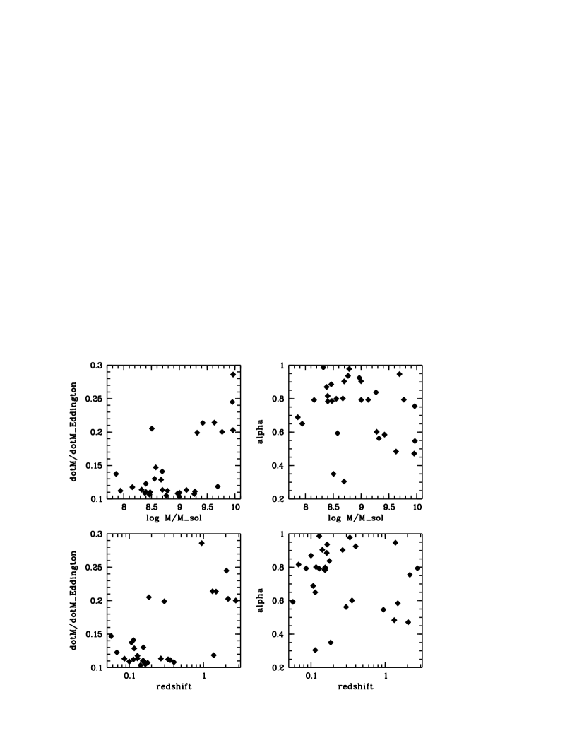
The resulting best fit parameters of all sample members, as well as their $1\sigma$ errors and the corresponding minimum $\chi^{2}$ values are given in Table 4. Cases where the upper or lower errors lie beyond the limit of our calculated grid, are denoted by a minus sign. In most cases acceptable fits are achieved. The distribution of model parameters was studied using a maximum likelihood technique (see Avni 1976) which, based on the assumption that both the model parameters and their statistical errors follow the normal distribution, gives the first (mean) and second moment (i.e., the $\sigma$ of the normal distribution) as well as their statistical errors. Figure 6 and 6 show the 68 %, 90 %, and 99 % confidence contours of the distribution of $\dot{M}$ and $\alpha$, respectively. The case that all sample members have the same $\dot{M}$ and/or $\alpha$ best-fit parameter values is excluded at a high statistical significance level (the confidence contours do not intersect the $\sigma=0$ line). We find a mean accretion rate of $<\dot{M}>\;=0.13\;\dot{M}_{\rm Eddington}$ within a relatively narrow parameter range ($\sigma\approx 0.05\;\dot{M}_{\rm Eddington}$). The best-fit accretion rates $\dot{M}$ are below $0.3\;\times$ the Eddington accretion rate in all sample members (see Fig. 8), thus fulfilling the requirement for the thin disk approximation (Laor & Netzer, 1989). The viscosity parameters are relatively high ($<\alpha>\;=0.76$) and are spread over a wider range ($0.5<\alpha<1.0$ for most objects), possibly suggesting some diversity of the underlying physical viscosity mechanism in our sample. Note that, according to its definition, $\alpha$ should not greatly exceed unity.

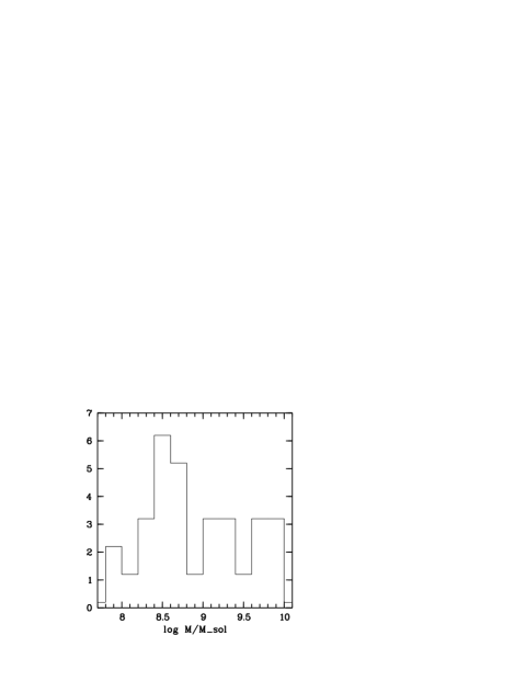
The best-fit central masses which roughly span two orders of magnitude ($10^{8}M_{\odot}-10^{10}M_{\odot}$; see Fig. 8) are in broad agreement with AGN black hole masses derived from variability and from general luminosity arguments. As the accretion rates are found to be confined within a relatively narrow range ($\dot{M}=0.1-0.3\times{M}_{\rm Eddington}$), this implies that, in absolute terms, the mass accretion rates also span about two orders of magnitude while maintaining a rough proportionality (within a factor $\sim 3$) with the central masses over the whole dynamic range. We have tested for any dependencies of $\dot{M}$ and $\alpha$ on $M$ and find that low central masses also seem to be associated with accretion at a lower fraction of the Eddington accretion rate, $\dot{M}/\dot{M}_{\rm Eddington}$: When $M$ is increased by two orders of magnitude (from $10^{8}M_{\odot}$ to $10^{10}M_{\odot}$) a moderate increase of $\dot{M}/\dot{M}_{\rm Eddington}$ by roughly a factor of three (from 0.1 to 0.3) is observed. No such dependence of the viscosity parameter $\alpha$ on central mass is observed. Scatter plots of $\dot{M}$ and $\alpha$ plotted over $M$ and redshift are shown in Fig. 9. High central masses also imply higher luminosities and, on average, larger distances. Any dependence on central mass thus is also expected to result in a similar dependence on redshift, as is observed (Fig. 9, lower panel). Note that the observed dependencies of $\dot{M}/\dot{M}_{\rm Eddington}$ on central mass and redshift can not be attributed to selection effects, alone: Objects with, e.g., central masses of $8\times 10^{8}M_{\odot}$ at a redshift of $z=0.1$ would be well above the respective X-ray and UV sensitivity limits if their mass accretion rates were higher than the observed values $<0.15\;\dot{M}_{\rm Eddington}$.

The narrow range of observed accretion rates in terms of the Eddington accretion rate also implies that the large luminosity range covered by AGN must predominantly be due to a similarly large variation in central mass. Note that for the object class studied here, i.e. radio-quiet quasars, the emission is considered to be dominated by an unobscured accretion disk and absorbing material on the line of sight is thus not thought to contribute to the large observed luminosity range. Taken together with the known evolution of the quasar luminosity function (e.g., Boyle et al., 1987 and 1993), i.e. the fact that quasars at high redshifts are considerably more luminous than ‘local’ quasars (by up to a factor of 40 at redshift z = 2, depending on which relative contribution of luminosity and/or density evolution is favoured) it follows that quasars at earlier epoches were more massive than present day quasars by similar factors, giving further support to the concept that many local galaxies (including our own; Genzel & Eckart, [1996]) contain dormant, super-massive black holes in their centers. See the more de 4 tailed discussion of this finding in Brunner et al. (1997).

We presently do not know which physical processes are responsible for the fact that high accretion rates (0.3 – 1.0 $\dot{M}_{\rm Eddington}$ for the total sample; 0.15 – 1.0 $\dot{M}_{\rm Eddington}$ for the low mass/low redshift subsample) are not observed. However, since the definition of the Eddington accretion rate is based on the assumption that both radiation and accretion flow are isotropic, suitable unisotropies of both the accretion flow and the resulting radiation may lead to a reduction of the permitted maximum accretion rates. Dynamical processes in the disk not considered in our present modeling may also result in a limit to the possible accretion rates. We believe that this highly interesting point warrants further theoretical attention. Note that the observed lower cutoff of the distribution of accretion rates ($\dot{M}\geq 0.1\;\dot{M}_{\rm Eddington}$) may be due to selection effects: At very low accretion rates no appreciable emission is expected in the X-ray range such that most objects will not be detected in the ROSAT band.

Figure 10: $\alpha_{\rm ox}$ plotted over accretion disk parameters, central mass $M$, accretion rate $\dot{M}/\dot{M}_{\rm Eddington}$, and viscosity parameter $\alpha_{\rm visc.}$. One anomalous object with the lowest $\alpha_{\rm ox}$ value in the sample is plotted as an open dimond.

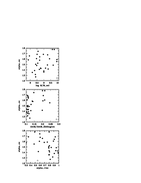
We find marginal correlations of the accretion disk parameters with $\alpha_{\rm ox}$ (see Fig. 10). When one anomalous object, # 20 (Table 1), with the lowest $\alpha_{\rm ox}$, and at the same time the highest $M(9.26\cdot 10^{9}M_{\odot})$ and $\dot{M}\;(0.286\;\dot{M}_{\rm Eddington}$) values in the sample is removed, the probabilities for randomness of the observed correlations of $\alpha_{\rm ox}$ on $M$, $\dot{M}/\dot{M}_{\rm Eddington}$, and $\alpha$ are 0.16, 0.04, and 0.02, respectively (Spearman rank correlation). Note that both $M$ and $\dot{M}/\dot{M}_{\rm Eddington}$ contribute to the total luminosity of the disk ($L\sim M\times\dot{M}/\dot{M}_{\rm Eddington}$). Since in the optical spectral range the emission is dominated by the accretion disk while at X-ray energies a large fraction of the emission is supplied by the hard power law component, an increase of either $M$ or $\dot{M}/\dot{M}_{\rm Eddington}$ predominantly affects the optical emission and thus results in an increase of the broad-band spectral index $\alpha_{\rm ox}$, in agreement with the observed correlations. By increasing the viscosity parameter $\alpha$ a larger part of the disk emission is radiated in the X-ray range, thus resulting in a hardening of the broad-band spectral index $\alpha_{\rm ox}$, again in agreement with observations.

A statistical comparison of the sample properties of AGN from the ROSAT All Sky Survey using a simpler precursor version of the present accretion disk code has been performed by Friedrich et al. ([1997]) which is in broad agreement with the present study. However, using the improved model, considerably smaller mass accretion rates are sufficient to produce the observed X-ray emission. This is mainly because, contrary to the simpler version, our improved model also takes into account the temperature gradient in the vertical direction of the disk. This means that the local spectra differ from the blackbody even in the optically thick case, leading to harder spectra for the same parameter values.

7 Concluding remarks

We are aware that the accretion disk model fitting performed leaves many open ends. I.e., contributions from other ingredients of the AGN phenomenon such as non-stationary processes in the disk, illumination of the disk, effects on the spectrum due to reflection and due to an absorbing torus have been neglected. However, the fact that in most cases acceptable fits of our accretion disk model were achieved has strengthend our belief that, for the objects selected, to first order this approach is justified. We thus have demonstrated that the ‘naked’ (excluding the above modifications) accretion disk model is a viable, and in fact we think the most promising candidate, for understanding the soft X-ray excess and big blue bump emission in at least some classes of AGN (radio-quiet quasars and Seyfert I galaxies). Further modeling including some of the above ingredients will, however, be highly desirable, particularly when considering the availability before the end of the century of X-ray instruments with much improved sensitivity, spectral resolution, and spectral coverage.