Star Cluster Ecology II:

Abstract

Three-body effects greatly complicate stellar evolution. We model the effects of encounters of binaries with single stars, based on parameters chosen from conditions prevalent in the cores of globular clusters. For our three-body encounters, we start with a population of primordial binaries, and choose incoming stars from the evolving single star populations of paper I. In addition, we study the formation of new binaries through tidal capture among the single stars. In subsequent papers in this series, we will combine stellar evolution with the dynamics of a full $N$-body system.

1 Introduction

In a dense stellar system, such as an open or a globular cluster or a galactic nucleus, encounters between individual stars and binaries can affect the dynamical evolution of the system as a whole. As a first step toward a more detailed description of such a stellar system, Portegies Zwart et al. (1997, hereafter paper I) modeled encounters and encounter products in a population of evolving single stars. In these calculations the stellar number density was held constant in space and time, as a first approximation to the collapsed core of a globular cluster.

As a second step we present in this paper the evolution of binaries in such a core, as follows. We add a single binary to the stellar system and follow its evolution until the binary is destroyed or ejected, or until the simulation terminates. This procedure is repeated to build up a large number of binary evolution histories. Thus we ignore in this paper encounters between binaries; we also ignore encounters between binaries and the products of binary evolution. A similar experiment was performed by [Davies 1995], but he neglected the detailed internal evolution of close binaries (see also the work of [Eggleton 1996]).

We consider both primordial binaries, formed simultaneously with the rest of the cluster, and tidal binaries formed later from encounters between single stars. Each binary evolves both through internal processes (e.g. the evolution of its components, stellar wind, mass transfer, etc.) and due to encounters with single stars.

The main purpose of this study is to gain a better understanding of the interactive processes between dynamics, stellar evolution and binary evolution. Our goal for the next episode in this series is to replace the integration of only 3-body systems with the full N-body evolution of the stellar system as a whole. The first pioneering experiments in this respect are performed by [Aarseth 1996].

The choices for the binary population in the cluster core, and the treatment of the internal evolution of the binaries and of encounters between stars and binaries are described in sect. 2. The results of our calculations are presented in sect. 3 and 4, for high- and low-density clusters, respectively. A brief preview of future work is given in sect. 5.

2 Methods

In this section we describe the various steps that take place in a single model calculation in which a population of binaries is evolved in a background of evolving single stars. In the present paper, we consider the limit of a low binary fraction: we model encounters between single stars and binaries, as well as those between single stars and single stars, but we neglect the occurrence of binary-binary encounters. The reasons for this choice are twofold. First, it is a good approximation to the core of a globular cluster in the asymptotic post-collapse regime, in which most primordial binaries have already been “burned up” ([McMillan & Hut 1994]). Second, it brings about a considerable simplification, in that it allows us to decouple the evolution of the single stars and the binaries.

As a first pass through the history of the star cluster, we follow only the single stars. We model the collisions between all types of single stars: both the primordial single stars, as well as the newly formed collision products. We thus model their internal stellar evolution, as well as their non-linear dynamical collision history (non-linear in the sense that doubling the density of stars will more than double the number of collisions per star, given the higher chance for collisions with and between the heavier collision products in the form of blue and yellow stragglers).

As a second pass, we model the collisions between single stars and binaries. As mentioned above, we limit ourselves to a strictly linear treatment, in the sense that each binary can encounter any of the single stars (primordial ones as well as stragglers), but is not allowed to meet another binary. Therefore, there is no need to evolve the binaries simultaneously. Instead, we simply decide how many binaries we would like to follow in total, and then evolve one binary at a time, until we have reached our quota.

Given the separability of the evolution of single stars and binaries, we can simply take the results of paper I to describe the former. For the binaries, we must (1) follow the internal changes caused by the stellar evolution of the individual binary member stars, (2) keep track of changes in the binary orbit caused by mass loss from, and mass exchange between, the two stars, and (3) model encounters between binaries and single stars.

Our overall approach is as follows. We start with a single-star environment taken from paper I, as described in sect. 2.1. In our “low-density” environment (model S below), collisions are rare and are modeled from the outset. However, in our “high-density” environment (model C), collisions are allowed only after a specific time $t_{\rm cc}$ (cc for core collapse), effectively using a step function to model the fact that collisions become important only during the later stages of dynamical evolution, around the time of core collapse.

We start the calculations in this paper by selecting one binary, as outlined in sect. 2.2. There are two possibilities, depending on whether this binary is primordial, formed together with the rest of the cluster, or a product of tidal capture, and thus formed at a later time. A primordial binary is evolved in isolation until the time $t_{\rm cc}$ (sect. 2.3), at which point it starts to interact with the single stars. In contrast, a tidal binary can only be formed at a later time, in our model, and we thus have to update our single-star environment to reflect this fact. In either case, we are then ready to implement dynamical three-body encounters between binaries and single stars chosen randomly from the appropriate distribution function.

In sect. 2.4, we describe the selection of these three-body scattering events. In a nutshell, we choose a time step, and determine whether or not the binary encounters a single star in this time step. If an encounter is indicated, we carry out the scattering operation, and we update both the binary and the stellar system, as detailed in sect. 2.5. We then choose a new time step, and repeat our Monte-Carlo selection procedure. This process is continued until the binary is destroyed or until the end of the dynamical calculation, whichever occurs first. We then select a new binary, repeat the whole binary evolution procedure, and continue until we have followed the required number of binaries. A list of terms used in our scattering experiments is provided in sect. 2.6.

2.1 The single star environment

We consider two stellar environments, one with a Salpeter type mass function and a moderate density which we call model $S$, and one with a mass function that is strongly affected by mass segregation and with a high density, appropriate for a post collapsed core, which we call model $C$. The relevant parameters of these models are given in Tables 1 and 2 (see also paper I).

We evolve the stellar system with single stars and collisions between them as described in paper I. Two stars are assumed to merge into a single object if they approach each other within a distance equal to the sum of their stellar radii (note that for paper I, twice this value was used; we discuss our reasons for making a different choice here in sect. 3.3). Binaries that pass each other at a slightly larger distance experience a tidal encounter, which might directly lead to coalescence. If the tidal encounter results in the formation of a binary, the orbital parameters of this binary are stored together with the mass and evolutionary state of the two stars in a data base of tidal binaries. Binaries of this type are evolved in a later pass, as described in sect. 2.2.1.

The stellar content of the cluster is stored in binned form (see sect. 3.4 of paper I) at regular time intervals $\Delta t$. The appearance of the stellar system between two stored moments $t$ and $t+\Delta t$ is determined by interpolating the number densities of the various stellar masses, radii and types linearly in time between those two instances. The environment of single stars is not affected by the binaries that are evolved within it; a collision product formed in a dynamical encounter between a single star and a binary is not added to the environment, and a single star that is destroyed (or exchanged) by an encounter is not discarded from the environment. With each bin, a single number is associated to indicate the number of stars at a given time interval, within the ranges in mass and radius corresponding to that bin. The identity of the individual stars is thus lost, in order to reduce the storage requirements for the single-star data base.

Whenever a binary is taken as a candidate for interaction with single stars, at time $t$, the single star environment is retrieved from the data base, and interpolated between the two storage times that straddle the time $t$. Having thus synchronized the single stars with the binary, we can determine whether an three-body encounter occurs (see sect. 2.4). If an encounter occurs between one of the retrieved stars and the binary, the current evolutionary state of the star has to be known. In the recovery process from the stored stellar mass, radius and type of a star, the individual age of the star is not known. In most cases, when the star is not affected by earlier collisions this poses no problem: the stellar age is equal to the age of the stellar system. Things are more complicated in case the star has been formed as a collision product. This implies that the star is relatively young compared to the stellar system. We assign an age for this rejuvenated star with the following procedure.

From the mass, radius and stellar type of a retrieved star its age can be uniquely determined. When a star is more massive than the other cluster members in the same evolutionary state, its implied stellar age is less than the age of the system as a whole. In order to know exactly how much smaller, we would have to know the identities of the progenitor stars, and the amount of mixing that has occurred during the merging process. The latter is still a matter of considerable debate, and the former is something we do not have access, since our binning erases specific information pertaining to individual stars. Therefore, we have adopted a simple recipe: we assume that the amount of mass in excess to a normal star in the same evolutionary state is accreted onto the rejuvenated star (see paper I for a discussion of this treatment).

This recipe will make some errors. For example, let us consider a globular cluster with a turn-off mass of $0.8\mbox{${\rm M}_{\odot}$}$. In this environment, if two $0.5\mbox{${\rm M}_{\odot}$}$ stars collide, they form a blue straggler with a total mass of $1\mbox{${\rm M}_{\odot}$}$. Our recipe will treat this system in the same way as a similar process in which a $0.2\mbox{${\rm M}_{\odot}$}$ star would have collided with a $0.8\mbox{${\rm M}_{\odot}$}$ star. In the latter case, the addition of $0.2\mbox{${\rm M}_{\odot}$}$ will only briefly delay the turn-off star in its ascent onto the giant branch. In contrast, the actual system, in which two equal-mass stars have collided, can be expected to live considerably longer, since both stars were still far from exhausting the hydrogen in their cores. Fortunately, in most cases the error made by our approximate treatment is relatively small, since the high-mass merger remnants typically have much smaller lifetimes than the age of the system (see Fig. 6 in paper I).

2.2 Initialization of the binaries

We consider the evolution of both primordial binaries and tidal binaries. Here we treat the initialization of each type of binary in turn.

2.2.1 Tidal binaries

To determine the formation properties of tidal binaries, we must first determine, at any given time, whether any two stars in the stellar system are about to undergo an encounter that is sufficiently close to offer the possibility of collisions or tidal capture. The calculation required is similar in many respects to the calculations carried out in paper I, where we studied encounters between single stars leading to collisional merging. In that paper, stars were assumed to merge when the distance of closest encounter $d$ between their centers was less than twice the sum of their radii: $d\leq 2(R_{1}+R_{2})$, where $R_{i}$ is the radius of star $i$. For purposes of computing tidal capture rates, we must consider larger $d$ values. As an upper limit for $d$, we have chosen $d_{\rm max}=5(R_{1}+R_{2})$. This is a safe upper limit for conditions under which tidal capture may occur.

As described in paper I, the velocity distribution of stars with mass $m$ is given by a Maxwellian, and therefore the distribution of relative velocities of two stars chosen at random are given by another Maxwellian, which we denote $F(v)$. The stars that are involved in an encounter are not chosen randomly, however: stars with lower relative speeds have considerably higher probability of becoming involved in an encounter. We take this into account by choosing the relative stellar velocity from a distribution $P(v)$ weighted by the encounter rate $\sigma v$, where $\sigma$ is the cross section for an encounter to occur:

$$P(v)dv=\sigma vF(v)dv.$$ (1)

The velocity distribution $P(v)$ (Fig. 1) depends on $d_{\rm max}$, through the dependence of the cross section $\sigma_{\rm max}=\sigma(d_{\rm max})$ on $d_{\rm max}$.

After choosing the relative encounter velocity from Eq. 1, the cross section $\sigma_{\rm max}$ for any encounter leading to stellar collision or tidal capture is

$$\sigma_{\rm max}=\pi d_{\rm max}^{2}\left(1+2G\frac{M_{1}+M_{2}}{v^{2}d_{\rm max}}\right),$$ (2)

where $M_{i}$ is the mass of star $i$ and $v$ is the relative velocity between the two stars at infinity.

The probability distribution for an encounter is linear in $\sigma$, by definition. Therefore, we can choose a random value for $\sigma$ from a flat distribution between 0 and $\sigma_{\rm max}$. We can then obtain the distance of closest approach $d$ by inverting $\sigma(d)$ (see Eq. 2 with $d$ substituted for $d_{\rm max}$, and $\sigma$ substituted for $\sigma_{\rm max}$) to obtain $d(\sigma)$.

Figure 1: Velocity distributions $P(v)$ for “interesting” encounters (i.e. leading to a physical stellar collision or to a significant binary perturbation) to occur, for the cases (a) two identical 1 ${\rm M}_{\odot}$, 1 ${\rm R}_{\odot}$ stars (solid line), and (b) a binary with a total mass of 1 ${\rm M}_{\odot}$ and a semi-major axis of 1 AU encountering a star with a mass of 1 ${\rm M}_{\odot}$ and a radius of 1 ${\rm R}_{\odot}$(dashed line). For comparison, the dotted line indicates the Maxwellian velocity distribution with a dispersion of $\sqrt{2}\mbox{${\rm v}_{\odot}$}$ (Eq. 4). The solid curve is arbitrarily normalized to a maximum value of unity; the areas under all three curves are the same.

The amount of energy deposited into oscillatory modes in the two stars at the moment of periastron passage is computed using the method described by Press & Teukolsky (1977, and refined by [Lee & Ostriker 1986], [McMillan et al. 1987], [Ray et al. 1987]; see also Mardling 1995a,b), where each star is taken to act upon the other as a point mass. The amount of energy dissipated in the tidal interaction is computed using the semi-analytic formulae provided by [Portegies Zwart & Meinen 1993]. These equations give, as a function of primary and secondary mass, radius and polytropic index $\gamma$ the total energy $E_{\rm tide}$ dissipated in the first periastron passage. For the computation of the amount of energy dissipated we use a polytropic index of $\gamma=3/2$ for all stars.

The final energy of the two-body system is calculated by subtracting the dissipated energy from the kinetic energy at infinity before the encounter. If the total energy is positive, no binary is formed, and the encounter is discarded. If the total energy is negative, the semi-major axis and eccentricity of the newly formed binary are calculated from the total energy and distance of closest approach $d$, assumed equal to the periastron distance of the new orbit. We then model the subsequent (partial) tidal circularization of the binary as an instantaneous process, as follows. We let the binary reduce its eccentricity under conservation of angular momentum until either of two types of outcome takes place. In some cases, the binary will become circular before the periastron distance has reached a value of four times the radius of the largest component. In other cases, this criterion will be reached for non-zero eccentricity. In both cases we freeze the binary, neglecting the remaining tidal interaction in the latter case (until stellar evolution effects increase the radii of the stars).

If one of the stars fills its Roche lobe after the binary has been circularized, the stars are merged and the encounter is classified as a collision. After the formation of a tidal binary, both stars are removed from the system of single stars and the orbital and stellar parameters of the binary, as well as the time of capture, are stored. Later, in the second pass in which we consider tidal binaries as candidates for three-body encounters with single stars, this stored information is retrieved to evolve the tidal binaries in the collisional environment.

2.2.2 Primordial binaries

The primordial binaries are initialized at zero age with distribution functions for the mass of the primary, the mass ratio, the semi-major axis and the eccentricity. All primordial binaries contain two main-sequence stars. The mass of the primary $M$ is taken from the mass function for the single stars (see paper I, sect. 3.1.1). After the primary mass is chosen, the mass $m$ of the secondary is selected, between the minimum mass of 0.1 ${\rm M}_{\odot}$ and the mass of the primary, from a specified probability distribution $\Phi(q)$, where the mass ratio $q=m/M$ is defined to be smaller than unity (see Table 1).

Table 1: Initial conditions for the primordial binaries for the low density model S, with a Salpeter primary mass function. The parameters are listed in the first column, the distribution function in the second, and the lower and upper limits are given for the models $C$ and $S$. A primordial binary that is not detached at zero age is rejected. Note that in model C the initial parameters listed here are substantially modified to take into account the effects of dynamical evolution prior to the start of the simulation at time $t_{cc}$. As a result, the initial mass function actually used in that model is considerably flatter than Salpeter.

		Models $S$ & C
Symbol	Function	min	max
$M$	$\Psi(M)\propto M^{-2.35}$	0.1${\rm M}_{\odot}$	100${\rm M}_{\odot}$
$q$	$\Phi(q)=$ const.	$0.1\mbox{${\rm M}_{\odot}$}/M$	1
$e$	$\Xi(e)=2e$	0	1
$a$	$\Gamma(a)\propto 1/a$	1${\rm R}_{\odot}$	10AU
criterion for survival:		detached

This procedure is biased, in that only the primary has been selected from the single star mass function, without any regard to the mass of the secondary. In model $C$, with a strongly segregated mass function, this treatment is not very realistic. Due to the large selection effects in observational analysis, it is not clear how we can best correct for this bias. Therefore we have adopted the following simple algorithm. We require that distribution of total masses of the resulting binaries follow the same probability distribution as the masses of the single stars. For the distribution of the single stars we use the mass function for the single stars in model $C$ (see paper I). A rejection technique is used to enforce this distribution, after first selecting a large number of candidate binaries.

The dispersion velocity of the center of mass of the binary is chosen according to equipartition:

$$v(M+m)=\sqrt{1\mbox{${\rm M}_{\odot}$}\over M+m}\mbox{${\rm v}_{\odot}$},$$ (3)

where ${\rm v}_{\odot}$ is the three-dimensional velocity dispersion for a 1${\rm M}_{\odot}$ star, for which we choose (see also paper I):

$$\mbox{${\rm v}_{\odot}$}=\sqrt{3}\times 10\mbox{km~{}s${}^{-1}$}\approx 17.3\mbox{km~{}s${}^{-1}$}.$$ (4)

The initial eccentricity distribution for a binary system is chosen to be thermal; $\Xi(e)=2e$ (see e.g. Duquennoy & Mayor 1991), with $0\leq e<1$. The initial semi-major axis is chosen from a distribution which is flat in $\log a$ (Kraicheva et al. 1978) with $a_{\rm min}\leq a\leq a_{\rm max}$. We choose $a_{\rm min}=1~{}\mbox{${\rm R}_{\odot}$}$ and $a_{\rm max}=$ 10 AU. After choosing the binary parameters we test whether the binary is detached; if not, one of the stars is filling its Roche-lobe, the binary is rejected and new parameters are chosen.

2.3 Internal evolution of the binaries

Our treatment for the internal evolution of a binary, including mass loss via stellar wind, mass transfer from one component to another, and other physical processes, follows the detailed description of model $AK$ from [Portegies Zwart & Verbunt 1996].

The description in [Portegies Zwart & Verbunt 1996] was mainly devoted to high-mass binaries and the treatment for accreting white dwarfs was rather imprecise. In the present context, accreting white dwarfs are quite common and a more refined treatment is appropriate. In observed novae the amount of mass accreted onto the white dwarf is generally smaller than the amount of mass ejected in a fast stellar wind (see e.g. [Livio & Truran 1992]). Mass dumped onto the white dwarf is not directly accreted by it, but rather temporarily stored a circumstellar disc or envelope. For a disc formed around a white dwarf after coalescence with a less massive star, we assume that the dwarf accretes at a rate equal to 1% of the Eddington limit and loses mass at a rate equal to the Eddington limit until the disc is lost. In the case of mass transfer onto a white dwarf from a binary companion, the disc/envelope accretes at a the Eddington limit and the white dwarf accretes at 1% of Eddington. When the accumulated mass in the envelope exceeds 1% of the total mass of the white dwarf a thermonuclear explosion expels the envelope. If the distance at pericenter is smaller than 1 ${\rm R}_{\odot}$, we consider the expelled mass to be discarded in a common envelope, decreasing the binary orbital separation. Otherwise, the material lost by the envelope is considered to be blown away in an isotropic stellar wind.

We define the internal evolution time limit of the binary $\tau_{\rm evb}$, as the time difference between the current time and the time at which one of the two stars will evolve into another evolutionary state. The categories we have chosen as signifying different evolutionary states are: main sequence, Hertzsprung gap, (sub)giant, horizontal branch, supergiant, as well as Wolf-Rayet and helium stars; see [Portegies Zwart & Verbunt 1996].

2.4 Initialization of three-body scattering events

The encounter rate between a given binary and all single stars in the stellar system is computed as follows.

We bin the stars in intervals of mass and radius (see sect. 3.4 in paper I). Within a bin, all stars share the same mass, radius and velocity dispersion. For each bin, we compute the probability for an encounter between stars from this bin and the binary.

The encounter probability between a representative star from a bin and the binary is determined through a procedure, similar to the one described above, in sect. 2.2.1. There, we used for the maximum distance of closest approach, $d_{\rm max}$, a value $d_{\rm max}=5(R_{1}+R_{2})$. Here, we can take the same expression, but we have to modify it in three ways.

First, we take as the “radius” of the binary its semi-major axis. Second, we can expect the need for a somewhat larger scaling factor, since we are interested in relatively mild interactions as well, in which the eccentricity may still be perturbed sufficiently to affect the binary noticeably. Finally, we must take into account the possibility that the incoming star is much heavier than the sum of the binary member masses, in which case a more distant encounter can still cause a significant perturbation on the binary. From the distance dependence of tidal interactions, it follows that the latter effect is proportional to the cube root of the mass of the single star.

After extensive trial runs, we found that the following expression of maximum value for the closest encounter distance was a safe choice:

$$d_{\rm max}=7(a+R_{3})\max\left(1,\left({M_{3}\over M_{1}+M_{2}}\right)\right)^{1/3}.$$ (5)

Here $R_{i}$ and $M_{i}$ are the radius and mass of the binary members (1 and 2) and of the incoming star (3), and $a$ is the semi-major axis of the binary orbit.

Following the procedure of sect. 2.2.1, with the above expression for $d_{\rm max}$, we can determine the partial cross section $\sigma_{sb}(v)$ for encounters between the binary and any of the stars from a given bin that lead to collisions or a non-negligible binary perturbation. Note that this partial cross section is still a function of the velocity $v$. In sect. 2.2.1 we choose the velocity through a rejection technique. In the present case, we have to integrate the equivalent of Eq. 1, to obtain the encounter rate $\Gamma_{sb}$ for any star from bin $s$ with the binary, given by

$$\Gamma_{sb}=n_{s}\langle\sigma_{sb}v_{sb}\rangle,$$ (6)

where the brackets indicate averaging over the velocity distribution which is taken to be a Maxwellian, and $n_{s}$ is the number density of stars from bin $s$.

The total encounter rate $\Gamma$ is obtained by summing over all single-star bins ($N_{bin}$ in total):

$$\Gamma=\sum_{s=1}^{N_{bin}}\Gamma_{sb}\equiv{1\over\tau_{\rm enc}}.$$ (7)

Here $\tau_{\rm enc}$ is introduced as a characteristic time interval between successive interesting encounters, between the given binary and all single stars.

At the beginning of each time step, we determine the distribution of stars over the bins and the number densities of stars in each bin, interpolating from the previous computations with single stars and compute the times scales for stellar evolution $\tau_{\rm ev}$ and collisions $\tau_{\rm enc}$. Here $\tau_{\rm ev}$ is the time difference between the current time and the next time at which the internal evolution of the binary is scheduled to be updated. The task of computing the sum over all bins $i$ in Eq. 7 is less daunting as may appear at first sight, as many bins contain no stars. This is illustrated in Fig. 4 below. The time step is then calculated as

$$\delta t=\min(0.05\tau_{\rm enc},\tau_{\rm ev},\tau_{\rm evb}),$$ (8)

to ensure that changes in the stellar population and in the binary are followed with sufficient resolution.

A rejection technique is used to keep track of collisions, as follows. We choose a random number between 0 and 1. If this number is larger than $\Gamma\delta t$, we conclude that no collision has occurred. We evolve all stars and the binary over a time interval $\delta t$, and continue with the next step. If the random number is smaller than $\Gamma\delta t$, a collision has occurred. In calculating the sum (Eq. 7) over the bins, we keep track of the partial sum after addition of each bin $i$, where the partial sum ranges over bins $1,2,...,i$. The first bin for which this growing partial sum exceeds the random number identifies the bin involved in the collision.

More than one stellar type may be found in a single mass-radius bin. For example, white dwarfs with a mass close to the Chandrasekhar limit and neutron stars can share a bin, and so can Thorne-$\dot{\mbox{Z}}$ytkow  objects and massive super giants. As mentioned earlier, the identities of individual stars are lost within each bin, but we keep track of the number of stars of each type. The actual type of star that is involved in the encounter is selected randomly from the bin with a probability proportional to the number of stars of each type in the bin.

2.5 Execution of three-body scattering events

Once a single star is selected, the initial conditions for the encounter with the binary are determined in a way similar to the selection procedure described in sect. 2.2.1. In particular, the relative encounter velocity between the binary and the single star is chosen randomly from the following distribution, corresponding to Eq. 9 (see Fig. 1):

$$P_{sb}(v)dv=\sigma_{sb}vF(v)dv.$$ (9)

The maximum impact parameter $p_{\rm max}$ follows from the defining relation $\sigma_{sb}=\pi p_{max}^{2}$, and the actual impact parameter value $p$ is determined randomly from a distribution flat in $p^{2}$.

After the relative velocity at infinity and the impact parameter have been chosen, the remaining parameters are taken randomly from their appropriate distributions (see [Hut & Bahcall 1983] and [McMillan & Hut 1996] for details). The three-body scattering event is then simulated, through explicit orbit integration, using the scatter3 module of the Starlab package developed by [McMillan & Hut 1996], which automatically determines the type of outcome of the scattering experiment.

If the incoming star emerges from the scattering process unchanged, leaving the binary behind in a new stable orbit, the scattering event is classified as a preservation encounter. If the outgoing star was originally a binary member, we designate the event an exchange reaction. In the case that all three stars emerge unbound, we speak of an ionization event; this can only occur when the total energy of the three-body system is positive. For negative total energy (that is, when the binary binding energy is larger than the kinetic energy at infinity of the relative orbit), a resonance scattering may occur, in which the three stars form a temporary bound state; such an interaction is characterized by multiple close encounters.

In addition to these outcomes, which can all occur in the point-mass limit, there are additional channels in our case, when stars have finite sizes. One possibility is that all three stars collide, leaving a single remnant. If two of the three stars collide, the remaining star can be either be unbound and escape, in which case we speak of a collision-ionization event, or it can remain bound in a new binary system with the merger remnant, in which case we speak of a collision-binary-formation.

We use the following notation to classify the outcome of a scattering event. The numbers 1, 2, and 3 indicate the primary and secondary of the binary, and the incoming star, respectively. Closed brackets are used to show that two stars form a binary. Braces designate a merger remnant, with the numbers within brackets indicating which of the stars were involved in the merger process. For example: an encounter that results in the formation of a new binary with the unaffected field star (3) in a binary with the merger product of the primary (1) and the secondary (2) is written as: $(\{1,2\},3)$; a triple merger is written as $\{1,2,3\}$; and ionization of the binary, leaving the third star unaffected, is written as $1,2,3$.

All encounters are computed in the center-of-mass frame of the three-body system. If, after the encounter, the center-of-mass velocity of the binary (assuming that a binary remains after the encounter) exceeds the escape velocity of the stellar system, then the binary is considered to escape from the system. Following the usual approximation, we take the escape velocity to be twice the velocity dispersion.

A soft binary, with a binding energy much smaller than the typical kinetic energy of a single star, is likely to become ionized through repeated encounters. This process of ionization often occurs after a large number of weak encounters, in which the binary is gradually pushed to higher and higher “energy levels” (wider orbits). To model this process in detail would require a large amount of computer time, and would not be very instructive. We therefore arbitrarily consider a binary to become ionized as soon as its apastron distance exceeds 10AU.

A collision between stars during the three-body encounter is assumed to occur whenever two stars approach each other to within a distance equal to the sum of their radii. We thus neglect tidal effects, which are relatively less important, given the competing three-body effects that prevent subsequent orbital circularization after what would have become a case of tidal capture if it had occurred in isolation. We also neglect mass loss during mergers: the mass of a merger remnant is taken to be the sum of the masses of the stars involved.

To give a reasonable prescription for the radius of the remnant star is a more difficult task, since the initial configuration of the remnant, while in dynamical equilibrium, will be far from thermal equilibrium, and therefore likely to extend well beyond its final relaxed size. For simplicity, we assign a merger product an initial radius that is equal to the sum of the radii of the two (or three) colliding stars, at least for the duration of the scattering experiment. This is a reasonable procedure, since the dynamical encounter takes place over a time interval that is negligible compared to both the thermal and the evolutionary time scales of the stars involved. As soon as the encounter is finished, we relax the structure and the evolutionary state of the merger remnants to their appropriate equilibrium configurations, according to the appropriate stellar evolution model (see paper I).

2.6 Terminology

Here we present a list of the main terms used in the present paper.

• Blue straggler: a main sequence star with a mass larger than the turn-off mass.
  

• Coalescence: the formation of a single object due to an unstable phase of mass transfer in a binary.
  

• Collision: result of a violent dynamical encounter between two or tree stars, leading to the formation of a single star.
  

• Exchange: a three-body encounter in which the incoming star replaces one of the binary components.
  

• Ionization: an event in which all stars involved emerge unbound. This can be the result of a supernova explosion, in the case of a two-body system, or it can occur as the result of a three-body encounter. It can also occur when a binary has become progressively wider, and finally reaches an apastron value exceeding 10AU.
  

• Merger: the outcome of a process involving two or three stars which either collide or coalesce.
  

• Yellow straggler: a (sub)giant with a mass larger than that of ordinary (sub)giants.
  

• Resonance: an intermediate state of a three-body encounter, in which all three stars are temporarily bound, and therefore undergo more than one close passage during the scattering process.
  

• Preservation: a three-body encounter in which the identity of the binary members remains unchanged.
  

Table 2: Parameters of the different model computations, and some resulting numbers. Columns specify the model, the core radius, the 3-dimensional velocity dispersion for a $1\mbox{${\rm M}_{\odot}$}$ star, the time at which encounters are started, the storage time interval, the stellar number density in the core, and the fraction of the true core that we simulate (for the computations with single stars only). For single stars we give the number of encounters per star [$\mbox{$\star$}^{-1}$] and the mean time between encounters (see also paper I); for binaries we list the average number of encounters per binary [$\mbox{$\star$}\mbox{$\star$}^{-1}$] and the mean time between encounters. For tidal binaries the mean time $\delta t_{tide}$ between capture events is also given.

							single stars		primordial		tidal capture
Model	$r_{\rm c}$	${\rm v}_{\odot}$	$t_{\rm cc}$	$\Delta T$	$\log n$	$f_{c}$	$n_{\rm enc}$	$\tau_{\rm enc}$	$n_{\rm enc}$	$\tau_{\rm enc}$	$\delta t_{\rm tide}$	$n_{\rm enc}$	$\tau_{\rm enc}$
	[pc]	[km/s]	[Gyr]	[Myr]	[$\star$ pc-3]		[$\mbox{$\star$}^{-1}$]	[Myr]	[$\mbox{$\star$}\mbox{$\star$}^{-1}$]	[Myr]	[Myr]	[$\mbox{$\star$}\mbox{$\star$}^{-1}$]	[Myr]
$S$	4.0	17.3	0	10	3.92	0.298	0.002	7.56	6.7	2300	14.0
$C$	0.1	17.3	10	5	6.64	8.750	0.258	5.81	33.6	26.6	9.28	11.5	80.9

3 Results for the high-density system

Because the effect of encounters is strongest in a dense cluster core, we first discuss the evolution of a population of primordial binaries in a stellar system with a relatively high number density of stars, and compare the results of this model with an identical population of primordial binaries that did not experience any encounters. The mass function for this high-density cluster core (model $C$, for “collapsed core”) is affected by mass segregation, causing it to be relatively flat. Therefore, for model $C$ we use equal numbers of stars per unit mass interval between 0.1 ${\rm M}_{\odot}$ and the maximum mass of a single star. For binaries, primary and secondary masses, semi-major axes and eccentricities are initialized as described in sect. 2.2.2 (see also Table 1).

In model $C$, dynamical encounters start at $t_{\rm cc}=10$ Gyr and the calculation is stopped at $16\,$Gyr. Single stars, forming the environment in which the binaries are evolved, were binned (in number density and relative density of stellar types, and masses and radii of the single stars) and stored at intervals of $\Delta t=5$ Myr (see Table 2 and sect. 2.1).

In sect. 3.1 we discuss the results of computations in which binaries evolve in isolation, without dynamical encounters. The evolution of primordial binaries that are allowed to encounter single stars are presented in sect. 3.2. The results for tidal binaries are discussed in sect. 3.3.

3.1 Primordial binaries without encounters

For the computation of primordial binaries without any encounters, a total of 50000 binaries are followed. It is convenient to define the fractional lifetime of a possible binary state [(ms, ms), (ms, gs), (gs, gs), etc., where the terms are defined in the caption of Table 3] as the total time that all binaries spend in that state divided by the total lifetime of all binaries. The average lifetime of a non-dynamically evolving binary is about 4.88 Gyr (from $t=10$ to 16 Gyr, see Table 3). Binaries that contain two main-sequence stars are, with a fractional lifetime of 90.0%, most common. On average, a binary spends 7.0% of its time as a main-sequence star with a white dwarf companion and 1.5% of the time with a (sub)giant. White-dwarf–white-dwarf binaries have a fractional lifetime of 1.3%. The remaining $\sim 0.2\%$ corresponds mainly to a (sub)giant accompanied by a white dwarf (see Table 3).

Table 4 gives the fraction of binaries that merge after an unstable phase of mass transfer. Overall, 9.3% of all binaries merge during the period of the calculation. Most mergers (82.2%) are the result of an unstable phase of mass transfer from a (sub)giant onto a main-sequence star. A considerable fraction of binaries survive this first phase of mass transfer, only to merge as soon as the main-sequence star in turn fills its Roche lobe and transfers mass onto the white dwarf. A small number of mergers (120 in total) originate from white-dwarf pairs ($50000\times 0.093\times 0.026$, see Table 4, second column), closely followed by merging main-sequence binaries (112 in total).

Figure 2: Hertzsprung-Russell diagram of a population of primordial binaries in model $C$, with no interactions with other cluster members, at a system age of 12 Gyr. Of the 5000 binaries we started with to produce this plot, 7.9% have coalesced in an unstable phase of mass transfer; the remainder survived. The axes are chosen to match the Hertzsprung-Russell diagram with encounters between single stars presented in paper I (see also [Portegies Zwart 1996]). The main-sequence and the (sub)giant branch are clearly visible, as is the second main-sequence extending to $\sim$0.75 magnitudes above the zero-age main-sequence. White dwarf binaries lie to the left with a color index of $B-V\la 0$. The few blue stragglers arise from internal binary evolution (stable mass transfer).

Figure 2 shows the Hertzsprung-Russell diagram at 12 Gyr of a population of 5000 primordial binaries in model C. (A fraction of the total number of binaries computed is chosen to facilitate comparison with the Hertzsprung-Russell diagrams of the other models.) The binaries at $B-V\sim 1.1$ – 1.4 and $M_{v}\sim 9$ – 10 (below the main sequence), contain a white dwarf and a low mass main-sequence star. In the absence of dynamical encounters, only a small number of blue stragglers are formed in the population of primordial binaries from model $C$ (see also Fig. 2). The majority of blue stragglers formed by binary evolution are the result of an unstable phase of mass transfer leading to coalescence; these single stars are not presented in Fig. 2; only blue stragglers formed by stable mass transfer appear on the diagram. From Table 4 we see that the majority of mergers occur between a main-sequence star and a (sub)giant, which does not lead to the formation of a blue straggler.

Figure 3: In the $\log a$ – $e^{2}$ plane, equal numbers of initial binaries are selected per unit area, with the exception of the upper left corner, where the periastron distance is unacceptably small. The numbers indicate for each location in this plane the fraction of primordial binaries in model $C$ that merge (top figure) or are ionized (bottom figure) relative to the maximum in that plane. The contours, at 12.5% intervals, follow the absolute number of events. The majority of binaries that end their lifetime as merged objects are found in the lower left corner of the semi-major axis – eccentricity plane, indicating that, as expected, binaries with short orbital periods and small eccentricities are more likely to merge, while binaries with initially large orbital separations are more likely to be ionized.

Table 3: Average lifetime of binaries in our models. The first row gives the average lifetime of all binaries (in Gyr). Subsequent rows give the fraction of this lifetime that an average binary spends in a particular phase. For example, a primordial binary in model $C$ spends 78.0% (693 Myr) of its time as a binary with two main-sequence stars (ms, ms). Abbreviations are as follows: ms: main-sequence star; gs: giant; wd: white dwarf; ns: neutron star; bh: black hole; we use $\star$ to mean any star, regardless of type. Note that we do not list Thorne-$\dot{\mbox{Z}}$ytkow objects, helium stars and Wolf-Rayet stars, nor do we discriminate between various evolutionary stages of (sub)giants, horizontal-branch stars and super giants.

binary	Model $C$			Model $S$
	non-d	prim	tide	non-d	prim
($\star$, $\star$)	4.88	0.892	0.928	15.58	15.62
($\star$, $\star$)	1	1	1	1	1
(ms, ms)	0.900	0.780	0.241	0.988	0.961
(ms, gs)	0.015	0.004	0.007	0.002	0.003
(ms, wd)	0.070	0.125	0.454	0.007	0.028
(ms, ns)	0.000	0.035	0.129	0.000	0.003
(ms, bh)	0.000	0.008	0.026	0.000	0.003
(gs, gs)	0.000	0.000	0.002	0.000	0.000
(gs, wd)	0.002	0.006	0.026	0.000	0.000
(gs, ns/bh)	0.000	0.001	0.009	0.000	0.000
(wd, wd)	0.013	0.017	0.030	0.002	0.001
(wd, ns)	0.000	0.011	0.022	0.000	0.000
(wd, bh)	0.000	0.006	0.017	0.000	0.000
(ns, ns)	0.000	0.004	0.005	0.000	0.000
(ns, bh)	0.000	0.003	0.007	0.000	0.000

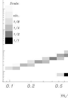
Figure 4: Relative encounter probabilities for a circular binary with total mass $1\mbox{${\rm M}_{\odot}$}$ and semi-major axis $1\mbox{{\rm AU}}$, as a function of the mass and radius of the other star involved in the encounter, for model calculation $C$ at time $t=12\,$Gyr, when the turn-off mass is $M_{\rm to}=0.91\,\mbox{${\rm M}_{\odot}$}$. Darker shades indicate higher probabilities. Compact stars (nominally with zero radius) are shown as a bar below 0.1 ${\rm R}_{\odot}$: neutron stars lie between 1.34 and 2 ${\rm M}_{\odot}$, white dwarfs and black holes lie at lower and higher masses respectively. All other stars with mass above the turn-off mass are products of previous encounters. The vertical bar at the upper left corner indicates the scaling. The lowest square corresponds to an encounter rate of one per 193 Myr, decreasing by a factor of two for each subsequent square. The integrated encounter frequency of the $1\mbox{${\rm M}_{\odot}$},1\mbox{{\rm AU}}$ binary is 1 encounter every 30.3 Myr. About 16% of the encounters occur with a $\sim 0.7\mbox{${\rm M}_{\odot}$}$ white dwarf (black square).

3.2 Primordial binaries with stellar encounters

A total of 5000 primordial binaries were initialized (see Table 1) and evolved in the dynamical stellar environment of single stars. The results of the scattering experiments performed on these binaries are summarized in Table 5.

3.2.1 Encounter outcomes

If a binary survives an encounter with another cluster member, its orbital elements, and possibly also its stellar components, are affected. Stellar evolution also affects these binary parameters. Both competing physical effects are computed simultaneously in order to follow the evolution of the binary population. The computation is terminated when a binary is dissociated, its components merge (without leaving the binary) or it escapes from the potential well of the stellar system after an encounter. Since a single binary can undergo multiple encounters, the total number of encounters is much larger than the initial number of binaries (see Table 2).

Table 6 presents the probabilities of the various binary termination channels. In the computation of the primordial binaries in model $C$, ionization is the dominant termination channel (see Table 6). A colliding encounter often results in the formation of a yellow straggler in a relatively wide binary. The size of the yellow straggler makes subsequent encounters a dangerous process, however, and a collision or an unstable phase of mass transfer can easily destroy the binary. The flat mass function allows many relatively massive, low-velocity stars to enter resonance encounters, and a considerable fraction of the primordial binaries collide or coalesce.

Table 4: Relative importance of various types of stellar collisions during dynamical encounters or mergers following an unstable phase of mass transfer. For each model we give the sum of the collision and coalescence rates (the total is normalized to unity) and the coalescence fraction. For non-dynamically evolving binaries (non-d), the coalescence rate is the total rate. Due to their small rates Thorne-$\dot{\mbox{Z}}$ytkow objects are not included, and triple collisions {$\star$, $\star$, $\star$} and mergers between two remnants {ns/bh, ns/bh} are not further specified. In some of the models the initial conditions do not allow certain stellar types to merge; this is indicated with a dash “–”. The total number of collisions per binary can be larger than unity (as is the case for the tidal binaries in model $C$), a new binary can be the result of a collision during a triple encounter.

		Model $C$					Model $S$
origin	non-d	primordial		tidal		non-d	primordial		tidal
	merged	merged	coal.	merged	coal.	merged	merged	coal.	coal.
per binary	0.093	0.571	25%	1.032	39.6%	0.094	0.116	16%	0.53
$n_{\rm merge}$	1	1	[%]	1	[%]	1	1	[%]	1
{ms, ms}	0.024	0.441	21	0.327	66	0.36	0.80	19	0.91
{ms, gs}	0.822	0.106	70	0.072	54	0.39	0.06	71	0.05
{ms, wd}	0.115	0.187	15	0.236	21	0.08	0.11	48	0.05
{ms, ns}	0.000	0.081	0	0.087	1	0.00	0.01	0	0
{ms, bh}	0.000	0.009	1	0.017	2	0.00	0.00	0	0
{gs, gs}	0.007	0.002	20	0.005	61	0.01	0.00	0	0
{gs, wd}	0.006	0.023	26	0.047	32	0.03	0.00	0	0
{gs, ns/bh}	0.000	0.015	3	0.027	11	0.00	0.00	0	0
{wd, wd}	0.026	0.046	70	0.055	77	0.13	0.02	100	0.1
{wd, ns/bh}	0.000	0.015	60	0.029	71	0.00	0.00	0	0
{ns/bh, ns/bh}	0.000	0.004	70	0.004	85	0.00	0.00	100	0
{$\star$,$\star$,$\star$}	–	0.071	–	0.104	–	–	0.01	–	0

Figure 3 shows the number of binaries, as a function of semi-major axis and eccentricity, that end their lifetime in a single object (upper panel), or that are ionized due to a dynamical encounter or by the dispersion criterion (lower panel). The initial conditions for all binaries are sampled homogeneously over the entire plane, with the exception of the upper left (small period and large eccentricity) corner. As expected, mergers occur more frequently in binaries with initially small orbital separations, while binaries with larger initial semi-major axes tend to be ionized. Near $a_{\rm max}$ the ionization fraction approaches 100%, indicating that our choice of maximum semi-major axis was large enough.

The total fraction of encounters leading to preservation is 95% (see Table 5). Only 11 non-preservation encounters resulted from encounters with an impact parameter exceededing 90% of the maximum impact parameter, confirming that our choice for the maximum impact parameter was large enough to ensure that not too many ‘interesting’ encounters are missed, and small enough to get reasonable statistics on unlikely encounters.

Only a small fraction ($\sim 1.8$%) of the preservations result from a resonant encounter (indicated in the third column of Table 5). Interactions where the primary is exchanged for the incoming field star [indicated as 1, (2, 3) in Table 5] are less than half as frequent as interactions where the incoming star takes the place of the secondary: 2, (1, 3). More than half of the secondary exchange encounters occur in resonances, whereas the majority ($\sim 70$%) of exchanged primaries are exchanged in prompt encounters. Note that only a small fraction of all encounters result in ionization. This is not surprising, since such an encounter can occur at most once per binary, while other interaction outcomes can occur many times (the same applies to collision-escape and triple collisions, to be discussed in the next paragraph).

Since the total number of collisions is rather small we normalize them separately to unity (see the lower part of Table 5). We subdivide the collisional encounters into (1) a collision (indicated by braces) and the subsequent formation of a binary (indicated by parentheses) (2) ionization (no parentheses) of the binary after the collision event and (3) the collision of all three stars, leaving a single object (braces). The collision–binary and collision–ionization events can both be further separated into three subclasses, depending on which two stars merge (see Table 5). Only a small fraction of triple mergers occur after a resonance encounter. This can be understood when one realizes that the incoming single star might well be comparable in size to the binary; a giant that encounters a close binary will collide with both binary components before having any chance to enter a resonant encounter.

3.2.2 Comparison with two-body collisions

Table 5: The results of dynamical encounters. For each possible outcome of a single scattering experiment (first column) the table gives encounter rates and the fraction (as a percentage) of encounters that were resonances. Data are presented for both primordial and tidal binaries, for high-density model $C$, and Salpeter model $S$. The total number of encounters $n_{\rm enc}$ for each model is normalized to 100. Hierarchical resonances are rare, and are combined with democratic resonances. The lower part of the table further subdivides the merging encounters, where for each model the total number of collisions is normalized to unity. Parentheses indicate a bound system, braces indicate a collision. A dash “–” indicates that this type of encounter is not possible. The total number of resonance preservation encounters per binary in model $C$ is 0.57 ($0.950\times 1.8\%\,n_{\rm enc}=1.7\%\,n_{\rm enc}$; $n_{\rm enc}=33.6$, from Table 2 with 5000 initial binaries).

	Model $C$				Model $S$
	primordial		tidal		primordial		tidal
	total	res.	total	res.	tot.	res.	tot.
$n_{\rm enc}$	100	[%]	100	[%]	100	[%]	100
(1, 2), 3	95.0	1.8	91.0	7.0	96.9	4	99.0
1, (2, 3)	0.9	30.8	0.8	58.1	0.6	51	0.0
2, (1, 3)	2.0	57.0	2.7	71.4	1.0	63	0.2
1, 2, 3	0.8	–	0.1	–	0	–	0.0
merged	1.3	47.4	5.4	44.7	0.1	27	0.8
merged:	1		1		1		1
(1, {2,3})	0.19	67	0.21	48	0.3	26	0.1
(2, {1,3})	0.18	61	0.19	49	0.4	51	0.5
(3, {1,2})	0.26	68	0.26	74	0.3	81	0.1
1, {2,3}	0.02	21	0.02	33	0.0	55	0.0
2, {1,3}	0.02	41	0.02	55	0.0	37	0.0
3, {1,2}	0.21	12	0.11	27	0.1	33	0.1
{1, 2, 3}	0.10	9	0.17	10	0.0	50	0.0

Table 6: Probability of various outcomes of a binary in the different model computations. The meanings of the terms used are explained in sect. 2.6.

origin	Model $C$		Model $S$
	prim	tidal	prim
preservation	0.144	0.215	0.955
ionization	0.599	0.110	0.017
collision	0.149	0.198	0.014
coalescence	0.058	0.387	0.018
escape	0.050	0.090	0.000

Figure 4 depicts the relative probability for a circular binary, with total mass 1 ${\rm M}_{\odot}$and semi-major axis 1 AU, to encounter a single star in the stellar system. Shaded squares indicate the binning used to improve performance, darker shades indicating higher encounter probabilities. A comparison between Fig. 4 and Fig. 3 of paper I reveal the effect of the larger size of the binary on the relative encounter probabilities: the binary encounter probabilities follow the relative densities of the various stellar species, whereas the probability distribution for the 1 ${\rm M}_{\odot}$single star from paper I is more strongly affected by a few individual stars with large interaction cross sections. Collision products formed during the previous evolution of the stellar system are present and can experience encounters with the binary. Blue and yellow stragglers are evident in Fig. 4 as stars with masses larger than $\sim 1$ ${\rm M}_{\odot}$ and with radii smaller and larger, respectively, than $\sim 2$ ${\rm R}_{\odot}$.

Figure 5: Relative merger frequencies (normalized to the total number of mergers) between various stellar species, from dynamical model $C$. The upper bar shows results for primordial binaries, the lower for tidal binaries. The abbreviation rm (for remnant) is used for both neutron stars and black holes.

Figure 5 visualizes the relative merger frequencies for the dynamically evolving model $C$. Comparison with Fig. 4 from paper I, which gives the relative collision frequencies between different stellar species in model $C$, shows a enhancement of the number of mergers between white dwarfs and other stars; other merger frequencies are suppressed. The small radii of white dwarfs mean that they are not favored in encounters between single stars. A white dwarf is considerably more likely to merge with another star during a binary interaction.

In paper I the only channel through which a blue straggler could form was a collision between two single stars. Although more than 20% of the stars in the high-density stellar system experienced a collision, the number of blue stragglers visible at any instant did not exceed about 3% (per star). The presence of primordial binaries provides an efficient channel of up to about 1% per binary for the formation of blue stragglers, either single or in binaries (see Fig. 8).

3.2.3 Comparison with binaries without encounters

Figure 6 shows the Hertzsprung-Russell diagram at 12 Gyr of the primordial binaries in model C with encounters. About 41% binaries survive the first 2 Gyr of dynamical evolution in the host stellar core. The objects at $B-V\sim 1.3$ and $M_{v}\sim 9$ – 10 (below the main sequence) are binaries comprising a low-mass main-sequence star and a white dwarf. There are very few giants among the primordial binaries—the majority of the binaries that are wide enough to contain a (sub)giant were destroyed in the first few hundred million years of the dynamical evolution of the stellar system. The large number of binaries still present at $t=12$ Gyr in Fig. 2 compared to the small number of binaries in Fig. 6 reveals that the primordial binaries that experience occasional encounters with other cluster members have a much shorter lifetime then the non-dynamically evolving binaries (see also Table 3, first row).

Figure 6: Hertzsprung-Russell diagram of a population of primordial binaries at a system age of 12 Gyr. The dots indicate binaries with visual magnitude smaller than 10 that survived the first 2 Gyr of dynamical evolution in model $C$. The scale is chosen to match the Hertzsprung-Russell diagram with encounters between single stars from paper I. The small number of binaries reflects their short lifetime. At this time, the main-sequence turn-off is around $M_{v}=4.5$, with $B-V\approx 0.7$ (effective temperature of 5500 K).

A “gap” between the turn-off of the stellar system and the more massive blue stragglers is visible in Fig. 6. This gap is not as obvious as the gap in Fig. 5 of paper I, but its origin is similar: The majority of all blue stragglers formed are the product of collisions. Because they tend to form from low-mass, relatively unevolved stars, and because their evolution time scales are long, blue stragglers just above the turn-off still lie close to the zero-age main sequence, as can be seen in Fig. 6. More massive blue stragglers evolve faster, and consequently have a broader distribution, extending from the zero-age main-sequence to the terminal-age main-sequence (see also [Portegies Zwart 1996]). In our models, the gap is largely the result of the dynamics (and hence most blue-straggler formation) being switched on at a specific time ($t_{cc}$). It is unclear to what extent this feature will persist in models with a more sophisticated treatment of the cluster dynamics.

Binaries evolving in a dynamical environment show a rich diversity compared to binaries that evolve non-dynamically (see Table 3). The formation of a binary containing a neutron star or a black hole is very rare in a non-dynamically evolving stellar system. However, the relatively large masses and small radii of these stellar evolution remnants make them excellent potential exchange partners in dynamical encounters. Once a massive remnant is exchanged into a binary, it is likely to be the more massive component, and not easily exchanged for another, lower mass, star (see Table 5). This results in a strong overabundance of binaries that contain at least one white dwarf, neutron star or black hole. An exchange interaction with a (sub)giant is not likely—the large radius of the giant generally leads to a collision with one or other of the stars during the encounter.

Table 4 illustrates how dynamical encounters dramatically enhance the probability of mergers (collisions as well as coalescence), and open the possibility of triple collisions. Although most merger rates are increased by dynamical encounters, the total number of {ms, gs} coalescence actually decreases considerably: 4.2% ($0.571\times 0.106\times 0.70$) versus 7.6% ($0.093\times 0.822$) for the non-dynamically evolving case. The reason is that binaries with orbital periods large enough to contain a (sub)giant have large cross sections for dynamical encounters, and tend to be destroyed before the primary has had time to ascend the giant branch.

Figure 7: Fate of binaries in Model $C$ as a function of time elapsed since the onset of dynamical encounters at 10 Gyr. The solid lines separate the possible outcomes for primordial binaries: preservation (i.e. binaries which either had no encounters or still are a binary following an encounter), merger (after Roche overflow or following a collision), ionization (disrupted by a supernova, dispersed because the separation at apocenter exceeds 10AU  or ionized by an encounter), and escape. For example, after $2\times 10^{8}\,$yr of encounters, $\sim 50$% of the primordial binaries remain, $\sim 5$% have merged, and $\sim 45$% have been ionized; $<1$% have escaped. The dashed lines indicate the same data for tidal binaries, where now “age” refers to time since the binary formed. As expected, the average lifetime of primordial binaries is much shorter than that of tidally formed binaries.

Figure 7 presents the overall evolution of the binary population, as a function of time since 10 Gyr (time $t_{cc}$, when the dynamical encounters were turned on). Note that half of the primordial binaries are destroyed within $\sim 100$ Myr.

3.2.4 Blue straggler evolution

We identify a blue straggler as a main-sequence star with a mass larger than the turn-off. In real clusters, it is generally hard to discriminate between main-sequence stars close to the turn-off and actual blue stragglers (also the identification of blue stragglers within the blue horizontal branch can be difficult in some cases). In our models, blue stragglers can be formed via number of different channels, leading to several distinct classes of stragglers—a single blue straggler can be formed by an unstable phase of mass transfer in a binary, or by a collision in a 2- or 3-body encounter. From Table 4, we see that most blue stragglers formed in model C are the result of dynamical encounters.

If a blue straggler is formed via a triple collision in a binary–single-star encounter, its mass will likely be considerably larger than that of most other blue stragglers in the stellar system. The lifetime of such high-mass blue stragglers (masses more than twice the turn-off mass, say) are very short, so their number at any moment is too small to contribute significantly to the overall population. The properties of blue stragglers formed by 2-body collisions between single stars are discussed in Paper I; the overall mass distribution of such blue stragglers is not significantly different when the collisions are mediated by primordial binaries.

Blue stragglers formed by unstable mass transfer generally have relatively small masses. Such a merger, and the subsequent formation of a blue straggler, can only occur via type $A$ mass transfer ([Kippenhahn & Weigert 1967]) when both stars are still processing hydrogen, which is unstable only if the mass ratio of the binary is small. The blue straggler thus formed is consequently slightly only more massive than the turn-off. Stable mass transfer leads to the formation of a considerably more massive blue straggler in a circular orbit around a Roche-lobe filling main-sequence star or a remnant from the mass-transfer phase (a helium star, white dwarf, or possibly a neutron star or a black hole). In our models, binaries containing a blue straggler and a mass-transfer remnant are often found to have a small eccentricity, induced by subsequent encounters with other stars. In contrast, a binary blue straggler formed by a collision during a 3-body encounter is generally highly eccentric, and the companion is not limited to a mass-transfer remnant or a Roche-lobe-filling star, but can be any type of star.

Figure 8: Number of blue and yellow stragglers formed in model $C$, with primordial binaries (dashed and solid lines, respectively) and with tidal binaries (dash-dotted and dash-dot-dot-dotted lines, respectively), as functions of time. The total number of tidal binaries is also shown (dotted line). All numbers are given as fractions of the total number of binaries modeled in the computations.

Figure 8 shows the numbers of blue and yellow stragglers in model C, as functions of time. During the first few million years of evolution in the high-density stellar system the numbers of blue and yellow stragglers rise steeply, eventually reaching equilibrium between formation and destruction of both types of objects. The fraction of yellow stragglers arrives at its maximum about 180 Myr after the onset of dynamical encounters. By this stage more than half of the original number of binaries have been destroyed, and the production rate of yellow stragglers decreases rapidly. At $t\approx 10.7$ Gyr only $\sim 35$% of the primordial binaries are still present in the stellar system (see Fig. 7), and the formation rate of blue stragglers becomes comparable to their destruction rate; the number of blue stragglers then starts to decrease and continues to do so until the end of the simulation. As blue stragglers evolve into yellow stragglers, the number of the latter increases again (from $t\approx 10.5$ Gyr) until the transformation of blue stragglers into yellow stragglers and the evolution of yellow stragglers into white dwarfs reaches equilibrium (at around 11.5 Gyr).

3.3 Tidal binaries in a dense cluster core

The rate at which close flybys between stars result in the formation of tidal binaries is only slightly smaller than the single-star collision rate (see Table 2). This can be understood by noting that the dominant term in the encounter cross section is linear in the distance of closest approach (due to gravitational focusing, see Eq. 2), and tidal capture is effective within a distance of roughly 3–4 times the radius of the larger star involved. Note that the collision rate between single stars (see Table 2) is smaller than computed in paper I. This is caused mainly by differences in the maximum periastron distance $d_{max}$ for which a physical collision can occur. As already discussed, in paper I we adopted a value of $d_{max}$ equal to twice the sum of the stellar radii, in an attempt to include (in an approximate way) tidal captures leading immediately to merging into the total collision rate. In this paper we take $d_{max}$ for collisions equal to the sum of the stellar radii, with a separate treatment of tidal capture. However, tidal binaries which begin Roche-lobe overflow directly after formation are also counted as collisions.

Capture between two remnants does not occur in our simulations, since both stars have nominally zero radius. The only way for a binary neutron star to form is via an exchange interaction, where an incoming neutron star replaces the companion of a neutron star already in a binary. If the exchanging binary has a short orbital period, the recoil velocity produced in the exchange interaction is generally large, and a considerable fraction of these interactions lead to escape of the neutron-star–neutron-star binary.

The initial conditions of tidal binaries differ from those of primordial binaries. Tidal binaries can be formed (a) at any moment between $t=t_{\rm cc}$ and 16 Gyr, (b) with arbitrary stellar types and masses at the moment of formation, and (c) with very small semi-major axes and eccentricities. The formation rate of tidal binaries is continuous from the instant when the stellar density reaches the value required for two-body encounters to become important until the end of the simulation. After an initial startup period of about 1 Gyr, the total number of tidal binaries remains roughly constant (see Fig. 8).

Initially there are no black holes in the stellar system, not even in the background single-star cluster: all black holes are formed from neutron stars that accrete sufficient material after a collision with another cluster member. This accretion process takes some time (about 1 Gyr), and the first tidal capture of a black hole by a main-sequence or giant star does not occur until $t=11.5$ Gyr. Black-hole tidal binaries are more common than black-hole primordial binaries (see Table 3), mainly because the number of targets for tidal capture is much greater than the number of surviving primordial binaries available for exchange.

Figure 9: The initial semi-major axes and eccentricities of 3000 tidal binaries with non-zero eccentricity, from model $C$. Dots, circles and squares indicate binaries containing a white dwarf and a main-sequence star, an early subgiant, and a horizontal branch star, respectively. The two squares at the right side of the figure are binaries with a white dwarf and a super giant. A subgiant spends most of its time at the bottom of the giant branch where its radius is smaller than that of a horizontal-branch star, for this reason the majority of the tidal binaries with a subgiant have a relatively small semi-major axis. The majority of tidal binaries are born with zero eccentricity and a short orbital period. (This statement, however, depends strongly on the algorithm adopted for their formation.)

The majority ($\sim 60$%) of tidal binaries have zero eccentricity. The distribution of the orbital parameters of the remainder, born with finite eccentricity, is illustrated in Fig. 9. The various stellar types that can capture a white dwarf populate different areas in the diagram. For each stellar type that captures a white dwarf, there is a minimum periastron distance for which successful (i.e. non-colliding) capture can occur. This is nicely demonstrated by the stars on the horizontal branch, all which have about the same radius. Note that this reflects the peculiarities of the algorithm adopted for the formation of tidal binaries; what nature does in these cases is unclear.

Because of their small orbital separations, relatively few tidal binaries are involved in encounters with other stars, and they are unlikely to become ionized when they do interact. Compared to primordial binaries, tidal binaries have long time intervals between encounters, and do not get ionized or exchanged so easily (see Table 6). Not surprisingly, those encounters that do occur have a larger fraction of resonance encounters, in which collisions are frequent (see Table 5 and Table 4). The majority of tidal binaries are destroyed by coalescence, collision or ejection from the stellar system (see Table 6 and Fig. 7). The half lifetime for tidal binaries (lower dashed line in Fig. 7) is more than twice as large as for the primordial binaries.

Due to their small encounter rates, tidal binaries are more strongly affected by stellar evolution than primordial binaries, and a larger fraction enter a phase of mass transfer. The merger rates (per binary) between main-sequence stars and (sub)giants, and between two main-sequence stars, are considerably smaller for tidal binaries than for primordial binaries (see Table 4), mainly because these stellar types are the dominant constituents of primordial binary systems. For all other types of binary the tidal-binary merger rate exceeds that for primordial binaries. The merger rate between two white dwarfs is enhanced due to the longer lifetime of the close binary, during which time gravitational radiation can reduce the orbital separation to the point of coalescence.

Figure 10: Hertzsprung-Russell diagram of a population of tidal binaries and single merger remnants, at a system age of (model $C$) of 12 Gyr.

Figure 10 shows the Hertzsprung-Russell diagram for the tidal binaries of model $C$ at a system age of 12 Gyr. The large diversity of objects is striking: blue stragglers as well as many yellow stragglers and white dwarfs are visible.

Figure 8 shows the numbers of blue and yellow stragglers as fractions of the total number of tidal binaries. After a few hundred million years of dynamical encounters, the blue and yellow straggler populations become important components of the stellar system. After about 2 Gyr of dynamical encounters, the numbers of blue and yellow stragglers reach equilibrium. The fraction of blue stragglers per tidal binary is roughly constant, at about 13%, over the full evolution time of the simulation, much larger than for single stellar collisions or a population of primordial binaries. The start-up time of about 1 Gyr can be understood from the knowledge that the mean tidal binary lifetime is about a Gyr (see Table 3 and Fig. 7).

Figure 11 illustrates the various destruction channels for a binary formed by the tidal capture of a main-sequence star by an evolved star (ms, gs) or a white dwarf (ms, wd). At the moment of destruction, a large fraction of all tidal binaries in our simulations still reflect their initial conditions. (This is not true for primordial binaries, whose appearance is changed dramatically by exchange or collision-binary interactions; see Tables 5 and 6). Collision and coalescence are common fates of tidal binaries, and the majority of the (ms, gs) binaries end their lives as single objects. Because of the smaller physical sizes of the stellar components, (ms, wd) binaries result are somewhat less likely to merge, and a larger fraction of these binaries escape or survive to the end of the calculation.

Once a white dwarf passes the Chandrasekhar limit, it is completely destroyed in a type Ia supernova, which dissociates the binary. The total supernova rate for tidal binaries is almost 0.08 supernovae per binary. Primordial binaries contribute for about 0.01 (supernovae per primordial binary) to the total type Ia supernova rate. In the core of a high-density stellar system, the total number of binaries formed by tidal capture can be estimated using the data given in Table 2. With these numbers, we arrive at a rate of about one type Ia supernova every 9.28 Myr$/0.08\simeq 120$ Myr. This is about 30% smaller than the supernova rate derived for single star encounters in paper I. The small contribution to the type Ia supernova rate from tidal binaries results from the capture frequency being smaller than the collision frequency.

Figure 11: Cannels (see text) by which a tidal binary is destroyed (model C), for two types of tidal binaries. The upper bar gives the relative frequencies of tidal binaries where a main-sequence star was captured by a (sub)giant or a main-sequence star. The lower bar indicates the relative frequency of captured white dwarfs. For details, see Table 6.

4 Results for the Salpeter mass function

In the model computation with a Salpeter mass function (model $S$ for Salpeter, see paper I and also Tables 1 and 2) we consider three different populations of binaries: 50000 non-dynamically and 5000 dynamically evolving primordial binaries, all initialized at $t=0$ (sect. 4.1, 4.2), and tidal binaries (sect. 4.3). The masses of the primaries are chosen between 0.1 ${\rm M}_{\odot}$and 100 ${\rm M}_{\odot}$, the other initial conditions are summarized in Table 1. Tidal binaries are initialized as described in sect. 3.2, but due to the small encounter rate in model $S$ (see paper I) only 1000 tidal binaries are modeled.

4.1 Primordial binaries without encounters

The steep mass function leads to many primaries having masses well below the turn-off, even at a system age of 16 Gyr. As a result, a large fraction of the non-dynamically evolving binaries of model $S$ do not reach Roche-lobe contact during the simulation. These binaries are listed as (ms, ms) binaries in Table 3. Binaries containing a Wolf-Rayet star are rare, both due to the small number of high-mass primaries, and to the short lifetimes of Wolf-Rayet stars. The total number of black holes and neutron stars is negligible; this is reflected in the low probability of finding one in a non-dynamically evolving binary (Table 3). A binary in which a neutron star is formed is likely to be dissociated by the asymmetry of the supernova, so few binaries contain neutron stars. (The distribution of kick velocities in our model is described with model $AK$ in Portegies Zwart & Verbunt 1996.)

The merger rate between white dwarfs is strongly enhanced in model $S$ relative to model $C$ (see Table 4). This is mainly a result of small differences in the initial mass-ratio distribution. Although the initial distributions are chosen identical (see Table 2) the adopted rejection technique tends to select equal mass pairs more often for model $S$ than for model $C$ (see sect. 2.2). These binaries are more likely to form (wd, wd) pairs which will subsequently emit gravitational waves, ultimately resulting in the merger between the two stars. The total number of white dwarfs (single as well as in binaries) in model $C$ is obviously higher than in model $S$ (see Table 3).

4.2 Primordial binaries with encounters

The encounter rate between single stars and primordial binaries is small, and due to the steep mass function, the majority of encounters involve low-mass main-sequence stars. The fractions of exchanges, collisions and resonance encounters are consequently small compared to those in model $C$. The majority of binaries survive to the end of the computation, and the average lifetime of a binary is almost as large as in the non-dynamically evolving case (see Table 3). Ionization is the second most important termination channel (see Table 6). The low encounter rate is reflected in the small difference between dynamically and non-dynamically evolving binaries (see Tables 3 and 4).

4.3 Tidal binaries

Because the low cluster density and small semi-major axes of tidally formed binaries results in very low encounter rates in model S, we have simply omitted these rates from Table 2. The majority of tidal binaries survive throughout the evolution of the stellar system without ever experiencing an encounter.

5 Outlook

This is the second paper in our star cluster ecology series. Our main aim is to provide stepping stones toward a full integration of stellar dynamics and stellar evolution for star cluster simulations. Paper I provided the first stepping stone: a treatment of collisions between single stars, drawn from a prescribed initial mass distribution and evolving independently between encounters. In the present paper we have taken the next step, incorporating a treatment of two more complicated processes: 1) the formation of binaries by tidal capture; 2) collisions between single stars and primordial binaries.

Subsequent papers in this series will apply the techniques that we have developed so far to full $N$-body systems. In these more realistic star cluster simulations, each star or binary, while unperturbed, will evolve according to the prescriptions given by Portegies Zwart & Verbunt (1996). The tools developed in this and the previous paper will enable us to model stellar evolution during periods of strong interactions.

In contrast to the following papers, the present paper is not meant to provide results that can be directly compared to observations. The approximations made are too extreme, and the initial conditions too simple, for such a comparison to be meaningful. The main aim of the present exercise is to give the reader confidence in and understanding of the techniques we have developed. The more realistic results from future papers in this series can then be checked and extended independently by others. Rather than providing black boxes for the dynamics and evolution of the stars in a cluster, our goal is to make the modeling procedure transparent.