A map for eccentric orbits in triaxial potentials

Abstract

We construct a simple symplectic map to study the dynamics of eccentric orbits in non-spherical potentials. The map offers a dramatic improvement in speed over traditional integration methods, while accurately representing the qualitative details of the dynamics. We focus attention on planar, non-axisymmetric power-law potentials, in particular the logarithmic potential. We confirm the presence of resonant orbit families (“boxlets”) in this potential and uncover new dynamics such as the emergence of a stochastic web in nearly axisymmetric logarithmic potentials. The map can also be applied to triaxial, lopsided, non-power-law and rotating potentials.

1 Introduction

The morphology of orbits in triaxial potentials determines the structure of triaxial galaxies. The simplest triaxial potentials are those of Stäckel form, which support four major families of regular orbits (boxes, short-axis tubes, and inner and outer long-axis tubes) and no stochastic orbits (Lynden-Bell 1962, de Zeeuw 1985). Many plausible triaxial potentials with smooth cores exhibit similar structure: most of phase space is occupied by these four major orbit families, with the leftover phase space hosting resonant minor families and stochastic orbits (Schwarzschild 1979).

Potentials without cores, such as triaxial logarithmic potentials of the form $\ln(\sum x_{i}^{2}/a_{i}^{2})$, can have quite different behavior (Gerhard & Binney 1985, Miralda-Escudé & Schwarzschild 1989). In this case the box orbits are replaced by a number of minor orbit families corresponding to various resonances. The minor orbits are centrophobic (center-avoiding) in contrast to the centrophilic box orbits, which all pass arbitrarily close to the center.

In special cases non-axisymmetric power-law potentials can have Stäckel form. Sridhar & Touma (1997) constructed planar, non-axisymmetric cuspy potentials which are separable in parabolic coordinates. These potentials remain separable if a central black hole is added. In the absence of a black hole, the dynamics are scale-free and all orbits belong to the centrophobic “banana” family. With a black hole, an additional family of centrophilic orbits (“lenses”) emerges to replace the box orbits of models with a smooth core.

The relevance of power-law potentials is enhanced by recent observations. High-resolution Hubble Space Telescope photometry of nearby elliptical galaxies and spiral bulges shows that the luminosity density near the center is a power-law, $\nu(r)\propto r^{\alpha-2}$ with $-0.3\mathbin{\lower 3.0pt\hbox{$\hbox to0.0pt{\raise 5.0pt\hbox{$\char 60\relax$}\hss}\mathchar 29208\relax$}}\alpha\mathbin{\lower 3.0pt\hbox{$\hbox to0.0pt{\raise 5.0pt\hbox{$\char 60\relax$}\hss}\mathchar 29208\relax$}}1.7$ (e.g. Gebhardt et al. 1996). Few or no galaxies have smooth cores ($\alpha=2$). There is also growing evidence for massive black holes in the centers of many nearby galaxies (Kormendy & Richstone 1995), which generate singular potentials that share many properties with the potentials generated by power-law densities.

We would like to understand how the orbit structure in non-axisymmetric power-law potentials $\propto r^{\alpha}$ changes with the exponent $\alpha$, and with the degree of non-axisymmetry. An exhaustive study with conventional integration methods is costly and difficult to interpret. We show how the dynamics of eccentric orbits in power-law potentials can be illuminated with the help of a symplectic mapping. The mapping models the evolution of such orbits as a two-step process: (i) precession of the orientation of the orbit in an axisymmetric potential; (ii) a kick to the angular momentum of the orbits at apocentre (where the star spends most of its time, and the torques are likely to be strongest). We use this mapping to study the orbital structure of non-axisymmetric power-law potentials over the range of $\alpha$ relevant to galaxies.

1.1 Scale-free spherical potentials

We assemble some properties of orbits in attracting spherical potentials of the form

$$\Phi_{\alpha}(r)=\left\{\begin{array}[]{cc}Kr^{\alpha},&\alpha\not=0,\\ K\ln r&\alpha=0.\end{array}\right.$$ (1)

where we assume henceforth that $-1\leq\alpha\leq 2$, which is true for most plausible potentials ($\alpha=-1$ is Keplerian; $\alpha=2$ is the harmonic oscillator; $\alpha=0$ is the singular isothermal sphere). Potentials with smaller $\alpha$ arise from density distributions with greater central concentration. We shall call potentials with $\alpha>0$ concave potentials and those with $\alpha<0$ convex. With no loss of generality we can set $K=\hbox{sgn}(\alpha)$ for $\alpha\not=0$ and $K=1$ for $\alpha=0$. The energy corresponding to a circular orbit with radius $r_{c}$ is then

$$E=\left\{\begin{array}[]{cc}{\textstyle{1\over 2}}|\alpha|r_{c}^{\alpha}+\hbox{sgn}(\alpha)r_{c}^{\alpha},&\alpha\not=0,\\ {\textstyle{1\over 2}}+\ln r_{c},&\alpha=0.\end{array}\right.$$ (2)

Note that $\hbox{sgn}(E)=\hbox{sgn}(\alpha)$ for all non-zero $\alpha>-2$, so that

$$|E|=\left(1+{\textstyle{1\over 2}}\alpha\right)r_{c}^{\alpha},\qquad\alpha\not=0.$$ (3)

The angular momentum of a circular orbit is

$$L_{c}(E)=\left\{\begin{array}[]{cc}|\alpha|^{1/2}\left(1+{\textstyle{1\over 2}}\alpha\right)^{-{\textstyle{1\over\alpha}}-{\textstyle{1\over 2}}}|E|^{{\textstyle{1\over\alpha}}+{\textstyle{1\over 2}}}\equiv h(\alpha)|E|^{{\textstyle{1\over\alpha}}+{\textstyle{1\over 2}}},&\alpha\not=0,\\ \exp\left(-{\textstyle{1\over 2}}\right)\exp(E)\equiv h(0)\exp(E),&\alpha=0.\end{array}\right.$$ (4)

Now consider motion in a plane and let $L$ be the scalar angular momentum, positive for prograde orbits and negative for retrograde orbits; it is convenient to work with the dimensionless angular momentum

$$y\equiv{L\over L_{c}(E)},$$ (5)

which can vary from $-1$ to $+1$. The orientation of an eccentric orbit can be specified by the azimuthal angle of its $n^{\rm th}$ apocenter, $\phi_{n}$. We may write

$$\phi_{n+1}=\phi_{n}+g(\alpha,y);$$ (6)

where the precession rate $g$ is independent of energy because the potential is scale-free, and $|g(\alpha,y)|$ is $2\pi P_{r}/P_{\phi}$, where $P_{r}$ and $P_{\phi}$ are the radial and azimuthal periods. The function $g$ is odd in $y$, and is given by

$$g(\alpha,y)=2h(\alpha)y\left\{\begin{array}[]{cc}\displaystyle\int{\displaystyle dr\over\displaystyle r[2\,\hbox{sgn}(\alpha)(r^{2}-r^{\alpha+2})-y^{2}h^{2}(\alpha)]^{1/2}},&\alpha\not=0,\\ \displaystyle\int{\displaystyle dr\over\displaystyle r[-2r^{2}\ln r-y^{2}h^{2}(0)]^{1/2}},&\alpha=0,\end{array}\right.$$ (7)

where the integral is over all radii for which the radicand is positive. For near-radial orbits we have

$$\lim_{y\to 0\pm}g(\alpha,y)\equiv\pm g_{0}(\alpha),$$ (8)

where

$$g_{0}(\alpha)=\cases{\pi,&for $\alpha\geq 0$,\cr{\displaystyle 2\pi\over\displaystyle 2+\alpha},&for $\alpha<0$.\cr}$$ (9)

When $|y|$ is small we have (cf. Appendix A)

$$g(\alpha,y)-g_{0}(\alpha)\sim|y|^{\beta},$$ (10)

where

$$\beta(\alpha)=\left\{\begin{array}[]{cc}1&1\leq\alpha<2,\\ \alpha&0<\alpha\leq 1,\\ -{\displaystyle 2\alpha\over\displaystyle 2+\alpha}&-\frac{2}{3}\leq\alpha<0,\\ 1&-1<\alpha\leq-\frac{2}{3}.\end{array}\right.$$ (11)

For near-circular orbits we have

$$\lim_{y\to\pm 1}g(\alpha,y)=\pm{2\pi\over(2+\alpha)^{1/2}},$$ (12)

which is the usual epicyclic approximation. There are two special cases for which the precession rate is simple,

$$g(\alpha,y)=\hbox{sgn}(y)\left\{\begin{array}[]{cc}\pi,&\alpha=2,\\ 2\pi,&\alpha=-1;\end{array}\right.$$ (13)

in addition, for $\alpha={2\over 3},1,-{1\over 2},-{2\over 3}$ the precession rate can be expressed in terms of elliptic functions (Whittaker 1959). In general $g(\alpha,y)$ cannot be determined in closed form, although an asymptotic series is given in Appendix A. A useful identity, easily derived from (7), is (Grant & Rosner 1994)

$$g(\overline{\alpha},y)=\left(1+{\textstyle{1\over 2}}\alpha\right)g(\alpha,y)\qquad\hbox{where}\qquad\alpha=-{2\overline{\alpha}\over 2+\overline{\alpha}};$$ (14)

thus the behavior of $g$ in the range $-1\leq\alpha<0$ is determined by its behavior in the range $0<\alpha\leq 2$.

Figure 1: Precession rate $g(\alpha,y)$ (eq. 7) as a function of dimensionless angular momentum $y$, for power-law potentials with exponent $\alpha=-0.8(0.2)1.8$. The precession rate is an odd function of $y$ and is only shown for $y>0$. Potentials with $\alpha<0$ are represented by dashed lines, those with $\alpha\geq 0$ by solid lines. The value of $g$ at $y=0$ (eq. 9) has been subtracted off; thus the analogous curves for $\alpha=-1$ and $2$ are zero everywhere (cf. eq. 13).

The map we discuss in the following section repeatedly employs the function $g(\alpha,y)$ at fixed $\alpha$. To minimize calculations of the integral (7) we tabulate $\log_{10}[g(\alpha,y)-g_{0}(\alpha)]$ at $\log_{10}(y)=-6(0.1)0$ and interpolate using a cubic spline. Computing this integral is straightforward but difficult to do well, in part because of the integrable singularities at the endpoints and in part because the endpoints themselves are determined implicitly; we can supply our program or results upon request. Figure 1 shows $g(\alpha,y)-g_{0}(\alpha)$.

2 A map for eccentric orbits

We now examine the behaviour of orbits in a scale-free axisymmetric potential that is perturbed by a small non-axisymmetric potential. If the unperturbed orbit is nearly circular, the behaviour can be analyzed using the epicycle approximation (e.g. Binney & Tremaine 1987, §3.3.3). Here we focus instead on an approximation valid for eccentric orbits.

In most cases the torques exerted by a non-axisymmetric potential on an eccentric orbit are concentrated near apocenter, since (i) the lever arm is larger; (ii) the particle spends most of its time near apocenter; (iii) any external tidal forces are stronger at larger radii.

Let $y_{n}$ and $\phi_{n}$ be the values of the dimensionless angular momentum and the azimuthal angle of a particle at its $n^{\rm th}$ apocenter passage. If the non-axisymmetric potential has $\exp(im\phi)$ symmetry then the time-integrated torque over the $n^{\rm th}$ apocenter passage can be written $-\epsilon L_{c}(E)\sin m\phi_{n}$; the minus sign is appropriate if the azimuthal minimum of the non-axisymmetric potential lies along the ray $\phi=0$. This torque induces a change in the angular momentum, of which half occurs before apocenter and half after; thus the dimensionless angular momentum after the particle leaves apocenter is

$$y_{n}^{\prime}=y_{n}-{\textstyle{1\over 2}}\epsilon\sin m\phi_{n}.$$ (15)

The position of the following apocenter is

$$\phi_{n+1}=\phi_{n}+g(\alpha,y_{n}^{\prime}),$$ (16)

and the angular momentum at this apocenter is

$$y_{n+1}=y_{n}^{\prime}-{\textstyle{1\over 2}}\epsilon\sin m\phi_{n+1}.$$ (17)

Equations (15–17) define a simple map $(\phi_{n},y_{n})\to(\phi_{n+1},y_{n+1})$ that describes the dynamics of eccentric orbits. The map is symplectic, like the exact equations of motion, and is more general than the exact equations because it does not depend on the specific radial form of the non-axisymmetric potential, so long as the torque is concentrated near apocenter.

2.1 Relation to the standard map

When $1<\alpha<2$ equations (8)–(11) imply that $g(y)\simeq\pi+Cy$ for $|y|\ll 1$, where $C$ is a constant (Fig. 1 shows how well this approximation holds). Thus the mapping (15)–(17) reduces to

$$y_{n}^{\prime} = y_{n}-{\textstyle{1\over 2}}\epsilon\sin m\phi_{n},$$

$$\phi_{n+1} = \phi_{n}+\pi+Cy_{n}^{\prime},$$

$$y_{n+1} = y_{n}^{\prime}-{\textstyle{1\over 2}}\epsilon\sin m\phi_{n+1}.$$ (18)

If in addition $m$ is even, we can change variables to $q=m\phi+\pi$, $p=mCy$, to get

$$p_{n}^{\prime} = p_{n}+{\textstyle{1\over 2}}K\sin q_{n},$$

$$q_{n+1} = q_{n}+p_{n}^{\prime},$$

$$p_{n+1} = p_{n}^{\prime}+{\textstyle{1\over 2}}K\sin q_{n+1},$$ (19)

where $K=mC\epsilon$. In this form, the map is the symmetric expression of the Chirikov-Taylor map, otherwise known as the standard map. This map serves dynamicists as a laboratory for examining the behavior of area-preserving maps as one increases the strength of perturbations. We refer the reader to the vast literature on the standard map (e.g. Lichtenberg & Lieberman 1992), and simply recall the transition to global stochasticity that occurs as $K$ exceeds the critical value of $\simeq 1$, or equivalently when

$$\epsilon\simeq\frac{1}{mC}.$$ (20)

Thus we expect that the map is regular when the non-axisymmetric perturbation is small, but only in the range $1<\alpha<2$. More specifically, we shall find below that when $\alpha<1$ near-radial orbits can exhibit a complex chaotic structure, even for arbitrarily small non-axisymmetric perturbations.

2.2 Non-axisymmetric potentials

We now ask what scale-free non-axisymmetric potentials can be generated by plausible density distributions. Scale-free density distributions can be written in the form

$$\rho({\bf r})=r^{\alpha-2}\sum_{\ell,m}a_{\ell m}{\rm Y}_{\ell m}(\theta,\phi).$$ (21)

The corresponding potential is (e.g. Binney & Tremaine 1987, §2.4)

$$\Phi({\bf r})=-4\pi Gr^{\alpha}\sum_{\ell,m}{a_{\ell m}{\rm Y}_{\ell m}(\theta,\phi)\over(\ell-\alpha)(\alpha+\ell+1)},\qquad-1-\ell<\alpha<\ell.$$ (22)

When $\ell=0$, the range of validity of equation (22) can be extended to all $\alpha>0$, since the dynamics are determined by the radial force $-d\Phi/dr$, which can be determined from (22) whenever $-1<\alpha$. Outside the range in which equation (22) is valid, the multipole potential is determined by the distribution of material at very large or very small radii, so that it satisfies Laplace’s equation and $\alpha=\ell$ or $-\ell-1$. Thus the range of potentials in which we are interested is given by

$$-1\leq\alpha, \ell=0,$$

$$-1-\ell\leq\alpha\leq\ell, \ell>0.$$ (23)

Since we restrict ourselves to the range of exponents $-1\leq\alpha\leq 2$, these constraints are always satisfied for monopole, quadrupole and higher multipoles ($\ell=0$ or $\ell\geq 2$). For dipole potentials ($\ell=1$), the constraints are only satisfied in the smaller range $-2\leq\alpha\leq 1$.

To assess the realism of the map, we shall compare trajectories in the map to orbits in scale-free non-axisymmetric potentials of the form

$$\Phi_{\alpha}(x_{1},x_{2})=\left\{\begin{array}[]{cc}\hbox{sgn}(\alpha)\left(x_{1}^{2}+{\textstyle x_{2}^{2}\over\textstyle b^{2}}\right)^{{\textstyle{1\over 2}}\alpha},&\alpha\not=0,\\ {\textstyle{1\over 2}}\log\left(x_{1}^{2}+{\textstyle x_{2}^{2}\over\textstyle b^{2}}\right),&\alpha=0,\end{array}\right.$$ (24)

where $x_{1}=r\cos\phi$ and $x_{2}=r\sin\phi$ are the usual Cartesian coordinates. The potential is specified by the exponent $\alpha$ and the axis ratio of the equipotentials, $b\leq 1$. The maximum angular momentum for an orbit of given energy now depends on the azimuthal angle $\phi$, and is given in terms of the maximum angular momentum in the analogous axisymmetric potential (eq. 4) by

$$L_{\rm max}(E,\phi)={L_{c}(E)\over\big{(}\cos^{2}\phi+\sin^{2}\phi/b^{2}\big{)}^{1/2}};\quad\hbox{thus}\quad|y|=\left|L\over L_{c}\right|\leq\big{(}\cos^{2}\phi+\sin^{2}\phi/b^{2}\big{)}^{-1/2}.$$ (25)

The map that approximates motion in this potential is specified by the same $\alpha$, azimuthal wavenumber $m=2$, and the torque amplitude $\epsilon$. To relate $\epsilon$ to the axis ratio $b\equiv 1-\delta$, we examine near-radial orbits ($y\ll 1$) in nearly axisymmetric potentials ($\delta\ll 1$). Then it is straightforward to show that to lowest order in $\delta$ and $y$

$${\epsilon\over\delta}=Q_{\alpha}\equiv\left\{\begin{array}[]{cc}\left(\textstyle 2\pi\over\textstyle\alpha\right)^{1/2}\left(1+{\textstyle{1\over 2}}\alpha\right)^{{\textstyle{1\over\alpha}}+{\textstyle{1\over 2}}}{\textstyle\Gamma(1+1/\alpha)\over\textstyle\Gamma({3\over 2}+1/\alpha)},&\alpha>0,\\ (2\pi e)^{1/2},&\alpha=0,\\ \left(\textstyle 2\pi\over\textstyle\beta\right)^{1/2}\left(1-{\textstyle{1\over 2}}\beta\right)^{{\textstyle-{1\over\beta}}+{\textstyle{1\over 2}}}{\textstyle\Gamma(-{\textstyle{1\over 2}}+1/\beta)\over\textstyle\Gamma(1/\beta)},&\alpha=-\beta<0.\\ \end{array}\right.$$ (26)

This ratio varies smoothly from $Q_{2}=\pi=3.1416$, to $Q_{0}=4.1327$, to $Q_{-1}=2\pi=6.2832$.

The map is based on the approximation that torques are concentrated near apocenter—that the intervals of the orbit when torques are exerted (mostly near apocenter) and when the orbit precesses (mostly near pericenter) are disjoint. This approximation is most accurate for nearly radial orbits—if the orbit is almost exactly radial then all of the precession occurs as the orbit passes the origin. If the non-axisymmetric component of the potential is given by (24), then the map is most accurate for concave potentials ($\alpha>0$), since in this case the torque is concentrated at large radii.

A second possible form for the potential is

$$\Phi_{\alpha}(x_{1},x_{2})=c(x_{2}^{2}-x_{1}^{2})+\left\{\begin{array}[]{cc}\hbox{sgn}(\alpha)\left(x_{1}^{2}+x_{2}^{2}\right)^{{\textstyle{1\over 2}}\alpha},&\alpha\not=0,\\ {\textstyle{1\over 2}}\log\left(x_{1}^{2}+x_{2}^{2}\right),&\alpha=0;\end{array}\right.$$ (27)

this form is not scale-free, but may be more natural if the non-axisymmetric potential arises from external tidal forces. For this potential the torques are always concentrated at large radii.

2.3 The logarithmic potential

We first apply the map to the logarithmic potential ($\alpha=0$), which is relevant to realistic galaxy models, and also represents a boundary between potentials in which near-radial orbits precess by $\pi$ in one orbit and those that precess by smaller angles (eq. 8). The behaviour of orbits in this potential has been examined by Richstone (1980, 1982), Binney & Spergel (1982), Gerhard & Binney (1985), Pfenniger & de Zeeuw (1989), and Miralda-Escudé & Schwarzschild (1989).

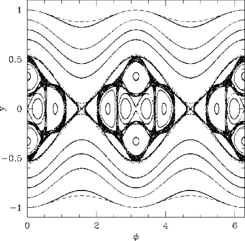
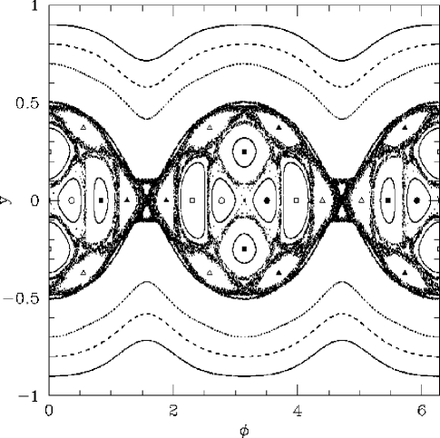
Figure 2: (a) Surface of section (SOS) for orbits in the potential (24), with axis ratio $b=0.88$. Each orbit is plotted for 1000 iterations, except for one stochastic orbit, which is plotted for 30,000 iterations to improve the definition of the stochastic web. The vertical axis is the dimensionless angular momentum (5) and the horizontal angle is the apocenter azimuth. The dashed lines show the maximum dimensionless angular momentum allowed by (25). (b) The map (15–17) with parameters $\alpha=0$, $m=2$, $\epsilon=0.5$. Resonant orbits of period 2 (“bananas”), 4 (“fish”), and 6 (“pretzels”) are marked by circles, squares, and triangles on the map; open and filled symbols denote different orbits.

Figure 2a shows the surface of section (SOS) for orbits in the potential (24) with $\alpha=0$ and $b=0.88$. The SOS shows the dimensionless angular momentum and azimuth each time the orbit passes through apocenter. The dashed lines show the maximum dimensionless angular momentum allowed by (25). The analogous map, with azimuthal wavenumber $m=2$ and dimensionless strength $\epsilon=Q_{0}(1-b)=0.5$, is shown in Figure 2b. The principal differences are: (i) the shapes of the regular orbits and the chaotic zones are slightly different; (ii) small resonant islands for near-circular orbits are present in the integration but not the map (between the last plotted orbit and the dashed boundary, centered on $\phi={\textstyle{1\over 2}}\pi,\frac{3}{2}\pi$); (iii) in the map there is no maximum angular momentum, so that some orbits continue to values of $|y|>1$ (these are not shown since they have no physical relevance). These differences are fairly minor, and mostly occur for near-circular orbits, for which the map was never intended to work well. Overall, the remarkable similarity of the two figures shows that the map correctly captures the qualitative dynamics of eccentric orbits in the logarithmic potential.

The SOS contains three main types of orbit:

• Loop orbits: these cross $\phi=0$ with angular momentum $|y|>0.5$. For each orbit sgn$(y)$ is fixed; that is, they circulate around the center in a fixed sense. The boundary of the loop orbits is defined by a separatrix that passes through the unstable fixed points at $\phi={1\over 2}\pi,{3\over 2}\pi$, $y=0$.

• Box-like orbits: Orbits with zero average angular momentum, which occupy a set of resonant islands inside the separatrix. The orbits are box-like because the apocenter azimuth librates around $\phi=0$ or $\pi$ and avoids $\phi={\textstyle{1\over 2}}\pi$ and $\frac{3}{2}\pi$. These orbits were examined by Gerhard & Binney (1985), Pfenniger & de Zeeuw (1989), and christened “boxlets” by Miralda-Escudé & Schwarzschild (1989). Each periodic boxlet has a signature which is the sequence of the signs of the angular momentum at successive apocenters ($+,-$ or 0). The periodic orbits at the centers of the major islands correspond to “banana” orbits (period 2, signature $[00]$), “fish” orbits (period 4, signature $[0+0-]$), and “pretzel” orbits (period 6, signature $[0++\,0--]$); the nomenclature is that of Binney (1982) and Miralda-Escudé & Schwarzschild (1989).

• A stochastic web, which shows up on the SOS as a connected fuzzy structure passing through $y=0$, $\phi={\textstyle{1\over 2}}\pi,\frac{3}{2}\pi$. Despite the complicated geometry of the web, this is a single orbit, which was followed for 30,000 iterations (compared to 1000 for the other orbits) to improve the coverage.

The SOS also provides preliminary information on which orbits are needed to construct self-consistent equilibrium galaxy models. The torques described by equation (15) with $m=2$, or the potential (24), are generated by a density distribution that is elongated along the axis $\phi=0,\pi$. The SOS shows that loop orbits are most eccentric when their apocenters are at $\phi={\textstyle{1\over 2}}\pi,\frac{3}{2}\pi$ and hence these do not support the required elongation of the density distribution. The box-like orbits, however, have apocenters that librate around $\phi=0$ or $\pi$ and avoid ${\textstyle{1\over 2}}\pi$ and $\frac{3}{2}\pi$; therefore these are aligned with the required figure. However, detailed studies of orbits in the logarithmic potential are required to determine whether the density distribution is narrow enough to allow self-consistent equilibrium models (Richstone 1980, Pfenniger & de Zeeuw 1989, Lees & Schwarzschild 1992, Kuijken 1993, Schwarzschild 1993).

Let us now consider the stochastic web in more detail. Because of the singularity in the logarithmic potential at $r=0$, we expect that any orbit passing close to the origin will be chaotic. In the context of the map, an orbit leaving the origin has zero angular momentum and azimuthal angle $\phi$; shortly before apocenter it receives an angular momentum kick $-{\textstyle{1\over 2}}\epsilon\sin m\phi$ (cf. eq. 15); therefore its phase-space coordinates at apocenter are

$$(\phi,y)=(\phi_{0},-{\textstyle{1\over 2}}\epsilon\sin m\phi_{0}).$$ (28)

All points in the map satisfying this constraint—and their iterates under the map—should belong to stochastic orbits. What is less obvious is that they all belong to the same orbit, i.e. that all orbits passing through the origin are part of the same stochastic web. We cannot prove this result but it is consistent with all of our numerical experiments with logarithmic potentials.

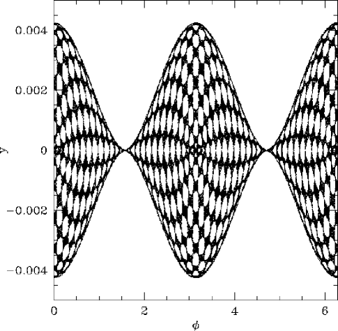
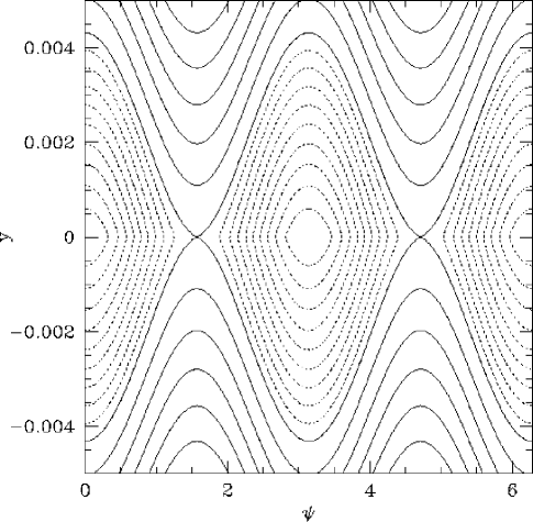
Figure 3: (a) A single stochastic orbit in the map (15–17) with parameters $\alpha=0$, $m=2$, $\epsilon=0.001$. The orbit has initial conditions $\phi={1\over 4}\pi$, $y=-0.0005$ (cf. eq. 28) and is iterated 100,000 times. (b) Level surfaces of the averaged Hamiltonian (32), for the same parameters as in (a). The variable $\psi$ equals $\phi$ or $\phi\pm\pi$. Level surfaces corresponding to loop orbits are shown by solid lines, and those corresponding to box-like orbits are shown by dotted lines.

The geometry of the web is particularly striking when $\epsilon$ is small. Figure 3a shows the web generated by 100,000 iterations of a single orbit in a map with $\alpha=0$, $m=2$, $\epsilon=0.001$. A very similar plot is generated by direct orbit integration in the analogous non-axisymmetric potential.

The following analysis provides some insight into the behavior shown in Figure 3a. Let $\psi_{n}=\phi_{n}-ng_{0}(\alpha)$ mod$(2\pi)$. Since $g_{0}(\alpha)=\pi$ for $\alpha\geq 0$, $\psi_{n}=\phi_{n}$ if $n$ is even and $\psi_{n}=\phi_{n}\pm\pi$ if $n$ is odd. Then for $m=2$ and $\alpha\geq 0$ equations (15–17) become

$$y_{n}^{\prime} = y_{n}-{\textstyle{1\over 2}}\epsilon\sin 2\psi_{n},$$

$$\psi_{n+1} = \psi_{n}+g(\alpha,y_{n}^{\prime})-g_{0}(\alpha),$$

$$y_{n+1} = y_{n}^{\prime}-{\textstyle{1\over 2}}\epsilon\sin 2\psi_{n+1}.$$ (29)

This mapping is equivalent to motion under the Hamiltonian

$$H=G(\alpha,y)-{\textstyle{1\over 2}}\epsilon\delta_{1}(t)\cos 2\psi=G(\alpha,y)-{\textstyle{1\over 2}}\epsilon\cos 2\psi\sum_{j=-\infty}^{\infty}\exp(2\pi ijt).$$ (30)

Here $\delta_{1}(t)=\sum_{k=-\infty}^{\infty}\delta(t-k)$ is the periodic delta-function with unit period, $t$ is a continuous variable which equals $n$ at the $n^{\rm th}$ iteration of the mapping, $y$ is the momentum conjugate to the coordinate $\psi$, $\psi(t=n)=\psi_{n}$, $y(t)=y_{n}^{\prime}$ for $n<t<n+1$, and

$$G(\alpha,y)=\int_{0}^{y}[g(\alpha,y)-g_{0}(\alpha)]dy.$$ (31)

If the motion is slow, the terms in (30) with $j\not=0$ have relatively little effect, and we can approximate the Hamiltonian by its averaged value

$$\overline{H}=G(\alpha,y)-{\textstyle{1\over 2}}\epsilon\cos 2\psi.$$ (32)

The motion is along level surfaces of this Hamiltonian, which are plotted in Figure 3b for the same values of $\alpha$ and $\epsilon$ as the map in Figure 3a. We see that the averaged Hamiltonian correctly captures the location of the separatrix and the division into loop orbits and box-like orbits (but not, of course, the detailed structure of the stochastic web).

2.4 The Liapunov exponent

The map can be used to determine the Liapunov exponent associated with the web for any value of the perturbation strength $\epsilon$. We simply follow the tangent map for an orbit that passes close to the center, i.e. one with initial coordinates given by equation (28). The tangent map is defined by taking differentials of equations (15–17):

$$dy_{n}^{\prime} = dy_{n}-{\textstyle{1\over 2}}m\epsilon\cos(m\phi_{n})d\phi_{n},$$

$$d\phi_{n+1} = d\phi_{n}+{\partial g\over\partial y}(\alpha,y_{n}^{\prime})dy_{n}^{\prime},$$

$$dy_{n+1} = dy_{n}^{\prime}-{\textstyle{1\over 2}}m\epsilon\cos m\phi_{n+1}d\phi_{n+1}.$$ (33)

The Liapunov exponent is

$$\lambda=\lim_{n\to\infty}{1\over n}\ln\left(d\phi_{n}^{2}+dy_{n}^{2}\over d\phi_{0}^{2}+dy_{0}^{2}\right)^{1/2}.$$ (34)

In practice we estimate the Liapunov exponent using large but finite $n$. Since we expect that all initial conditions (28) lie in the web (i.e. they are all the same orbit), the Liapunov exponent should be independent of the initial azimuth $\phi_{0}$.

Figure 4: The Liapunov exponent $\lambda$ (eq. 34) as a function of perturbation strength $\epsilon$, for maps with $\alpha=0$ and $m=2$. The initial conditions were taken from (28) with $\phi_{0}$ chosen randomly in $[0,2\pi)$. The perturbation strength $\epsilon$ was also chosen at random, from a uniform distribution in $\log\epsilon$ between $-4$ and $-0.5$. A total of 500 ($\phi_{0},\epsilon)$ pairs were examined, and each was iterated $10^{5}$ times.

Figure 4 shows the Liapunov exponent $\lambda$ for maps with $\alpha=0$ and $m=2$. The initial azimuth $\phi_{0}$ was chosen randomly in the interval $[0,2\pi)$ and each map was iterated 100,000 times. Although there are some outliers, in general the scatter is small, confirming that $\lambda$ is almost independent of $\phi_{0}$. What is unexpected is that $\lambda$ depends only weakly on the perturbation strength $\epsilon$—from around 0.07 near $\epsilon=0.3$ to $0.02$ near $\epsilon=10^{-4}$.

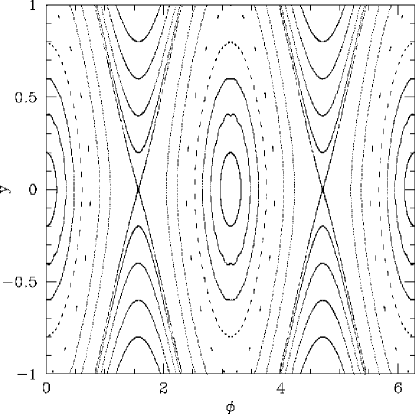
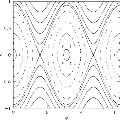
                                $(a)$ $(b)$

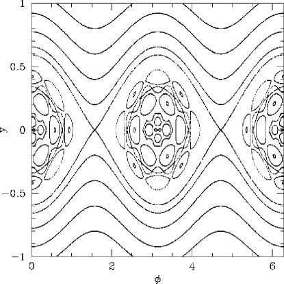
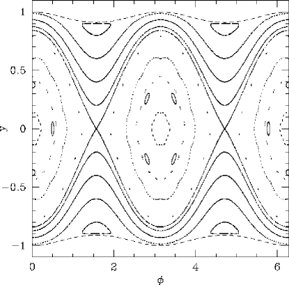
                                $(c)$ $(d)$

Figure 5: The map (15–17) with parameters $m=2$, $\epsilon=0.3$, and (a) $\alpha=1.5$; (b) $\alpha=1$; (c) $\alpha=0.5$. The orbits have been iterated 1000 times, except for the orbits at the separatrices, which are iterated 5000 times to provide better coverage. (d) The SOS for orbits in the potential (24), with $\alpha=1$ and axis ratio $b=0.91$ (cf. eq. 26). The dashed lines show the maximum dimensionless angular momentum allowed by (25). Each orbit is plotted for 1000 periods, except for the separatrix orbit, which is plotted for 5000 periods.

3 Concave potentials ($\alpha>0$)

The maps with $m=2$, $\epsilon=0.3$ and $\alpha=1.5,1,0.5$ are shown in Figure 5a,b,c. Like the map for the logarithmic potential examined already, these exhibit three types of orbits: loop orbits, which have a fixed sign of angular momentum; box-like orbits, which have zero average angular momentum and an apocenter azimuth that librates about $\phi=0$ or $\pi$; and a separatrix orbit, which passes through $y=0$, $\phi={\textstyle{1\over 2}}\pi,\frac{3}{2}\pi$ and separates the loop orbits from the box-like orbits.

Panel (d) shows the SOS for orbits integrated in the potential (24) with $\alpha=1$, $b=0.91$, which corresponds to the map (b). The similarity of the map in panel (b) to the SOS in panel (d) confirms that the map captures the qualitative dynamics in the non-axisymmetric potential. The principal difference, apart from minor changes in orbit shape, is the small resonant islands for near-circular orbits that appear in the integration but not the map (near the dashed boundary, centered on $\phi={\textstyle{1\over 2}}\pi,\frac{3}{2}\pi$).

The locations of the separatrices are well-described by the averaged Hamiltonian (32), as illustrated in Figure 6.

Figure 6: Separatrices of the averaged Hamiltonian (32), for $m=2$, $\epsilon=0.3$, and $\alpha=1.5,1,0.5$. These agree well with the locations of the separatrix orbits in the corresponding maps, panels (a),(b),(c) of Figure 5.

There are two interesting transitions in the behaviour of the box-like orbits as $\alpha$ is varied: (i) In Figures 5a,b ($\alpha\geq 1$) most of the box-like orbits form smooth curves surrounding the points $y=0$, $\phi=0,\pi$, while in Figures 5c and 2 ($0\leq\alpha<1$) the box-like orbits are almost all broken up into resonant islands. Miralda-Escudé & Schwarzschild (1989) call orbits of the first type “normal boxes” and those of the second type “boxlets”. Presumably this transition reflects the validity of the standard map as an approximation to the present map when $\alpha>1$ (§2.1). (ii) In Figure 2 the separatrix orbit is part of a stochastic web that surrounds all of the resonant islands, while in Figure 5c the separatrix orbit does not penetrate between the islands. Presumably this difference arises because KAM surfaces divide the separatrix from the islands in the latter case.

In §2.1 we argued that for $1\leq\alpha<2$, the mapping resembles the Taylor-Chirikov map, with the critical $\epsilon$ for global stochasticity given in equation (20). Thus the motion should be nearly regular for small $\epsilon$, in agreement with the phase portraits shown in Figures 5a,b and d.

3.1 A simpler map

The behavior of box-like orbits in concave potentials can be clarified by examining a simpler map. We begin with the map (29) and assume that $\psi$ is small, so that $\sin 2\psi_{n}\simeq 2\psi_{n}$. We also replace $g(\alpha,y)-g_{0}(\alpha)$ by its asymptotic form for small $y$ (eqs. 10 and 11). Thus we may write

$$y_{n}^{\prime} = y_{n}-\epsilon\psi_{n},$$

$$\psi_{n+1} = \psi_{n}+C\,\mbox{sgn}(y_{n}^{\prime})|y_{n}^{\prime}|^{\beta},$$

$$y_{n+1} = y_{n}^{\prime}-\epsilon\psi_{n+1}.$$ (35)

where $C>0$ is a constant and $0<\beta<1$. We now re-scale the coordinates, choosing new variables $I\equiv(\epsilon C)^{1/(\beta-1)}y^{\prime}$ and $\theta\equiv\epsilon(\epsilon C)^{1/(\beta-1)}\psi$. In these coordinates the map takes the simpler form

$$I_{n}^{\prime} = I_{n}-\theta_{n},$$

$$\theta_{n+1} = \theta_{n}+\mbox{sgn}(I_{n}^{\prime})|I_{n}^{\prime}|^{\beta},$$

$$I_{n+1} = I_{n}^{\prime}-\theta_{n+1},$$ (36)

The motion is governed by the Hamiltonian

$$H=\frac{|I|^{\gamma}}{\gamma}+{\delta}_{1}(t){\theta}^{2},$$ (37)

where ${\delta}_{1}(t)$ is the periodic Dirac delta function with unit period, $\gamma=\beta+1$, $\theta_{n}$ is the value of $\theta(t)$ at $t=n$, and $I_{n}^{\prime}$ is the value of $I(t)$ for $n<t<n+1$. We consider first the time-averaged Hamiltonian

$$H_{0}=|I|^{\gamma}/\gamma+{\theta}^{2}$$ (38)

The corresponding phase-space portrait consists of closed curves that are not differentiable on the axis $I=0$. With each trajectory we associate the action:

$$J = \frac{1}{2\pi}\oint Id\theta$$ (39)

$$= \frac{{\gamma}^{\frac{1}{\gamma}}W_{\gamma}}{\pi}H_{0}^{\frac{\gamma+2}{2\gamma}},$$

where $W_{\gamma}={\int}_{-1}^{1}{(1-x^{2})}^{\frac{1}{\gamma}}dx=\pi^{1/2}\Gamma(1+1/\gamma)/\Gamma(\frac{3}{2}+1/\gamma)$. The energy is simply given by: $H_{0}(J)=\omega_{0}J^{\frac{2\gamma}{\gamma+2}}$, with

$$\omega_{0}={1\over\gamma^{\frac{2}{\gamma+2}}}\left(\frac{\pi}{W_{\gamma}}\right)^{\frac{2\gamma}{\gamma+2}}.$$ (40)

Note that the frequency $\omega(J)=dH_{0}/dJ$ diverges as $J$ tends to zero, since $\gamma=\beta+1<2$. This feature implies that the motion is highly unstable near the origin once we add the high-frequency terms of the periodic delta function.

The transformation to action-angle variables is accomplished with the generating function

$$S(\theta,J)=\gamma^{\frac{1}{\gamma}}\int^{\theta}{\big{[}H_{0}(J)-\theta^{2}\big{]}}^{\frac{1}{\gamma}}d\theta,$$ (41)

which naturally gives the angle conjugate to $J$, $\phi=\partial S/\partial J$.

Now we restrict ourselves to the case $\beta=\gamma-1\ll 1$, which is valid for potentials that are close to the logarithmic potential. We have $\gamma\simeq 1$, $H_{0}(J)=\omega_{0}J^{2/3}$, $\omega_{0}=(3\pi)^{2/3}2^{-4/3}$. We can also write $\theta=(dH_{0}/dJ)^{-1}g(\phi)$, where $g(\phi)$ is the $2\pi$-periodic sawtooth function defined by

$$g(x)=\cases{x,&$|x|\leq{\textstyle{1\over 2}}\pi$,\cr\pi-x,&${\textstyle{1\over 2}}\pi\leq x\leq\frac{3}{2}\pi$,\cr g(2\pi+x).\cr}$$ (42)

In the action-angle variables $(J,\phi)$ of the averaged Hamiltonian, the mapping Hamiltonian becomes

$$H=H_{0}(J)+[\delta_{1}(t)-1]\left(dH_{0}\over dJ\right)^{-2}g^{2}(\phi)=H_{0}(J)\left\{1+{4\over\pi^{2}}[\delta_{1}(t)-1]g^{2}(\phi)\right\}.$$ (43)

We would like to analyze the principal resonances of this Hamiltonian. After Fourier expansion of $g$ and $\delta$, the Hamiltonian takes the form

$$H=H_{0}(J)\left[1+\frac{2}{3}\sum_{n=1}^{\infty}\cos(2\pi nt)+\frac{4}{{\pi}^{2}}\sum_{m\not=0}\sum_{n=1}^{\infty}\frac{(-1)^{m}}{m^{2}}\cos 2(m\phi-\pi nt)\right].$$ (44)

Choosing a resonant pair $(m,n)$, and including all terms of the form $(pm,pn)$, we end up with the resonant Hamiltonian:

$$H_{mn}=H_{0}(J)\left[1+\frac{4}{{m^{2}\pi}^{2}}\sum_{p=1}^{\infty}\frac{(-1)^{pm}}{p^{2}}\cos 2p(m\phi-\pi nt)\right].$$ (45)

We change coordinates with the canonical transformation: $F(J^{\prime},\phi)=2J^{\prime}(m\phi-\pi nt)$, giving $J=2mJ^{\prime}$ and ${\phi}^{\prime}=2(m\phi-\pi nt)$, and end up with the one degree of freedom Hamiltonian

$$H^{\prime}_{mn}(J^{\prime},\phi^{\prime})=H_{0}(2mJ^{\prime})\left[1+\frac{4}{{m^{2}\pi}^{2}}\sum_{p=1}^{\infty}\frac{(-1)^{pm}}{p^{2}}\cos(p\phi^{\prime})\right]-2\pi nJ^{\prime},$$ (46)

which simplifies to

$$H^{\prime}_{mn}(J^{\prime},\phi^{\prime}) = H_{0}(2mJ^{\prime})\left[1+\frac{2}{3m^{2}}-\frac{2\phi^{\prime}}{m^{2}\pi}+\frac{{\phi^{\prime}}^{2}}{m^{2}\pi^{2}}\right]-2\pi nJ^{\prime},\quad\hbox{$0\leq\phi^{\prime}<2\pi$, $m$ even}$$ (47)

$$= H_{0}(2mJ^{\prime})\left[1-\frac{1}{3m^{2}}+\frac{{\phi^{\prime}}^{2}}{m^{2}\pi^{2}}\right]-2\pi nJ^{\prime},\qquad\quad\hbox{ $-\pi\leq\phi^{\prime}\leq\pi$, $m$ odd}.$$

This Hamiltonian has equilibria at $0$ and $\pi$. For $m$ even and $\gamma\simeq 1$ we get

$$J_{0} = \left[2m\gamma\omega_{0}\big{(}1+\frac{2}{3m^{2}}\big{)}\over\pi n(\gamma+2)\right]^{\frac{2+\gamma}{2-\gamma}},$$

$$J_{\pi} = \left[2m\gamma\omega_{0}\big{(}1-\frac{1}{3m^{2}}\big{)}\over\pi n(\gamma+2)\right]^{\frac{2+\gamma}{2-\gamma}};$$ (48)

and for $m$ odd, $J_{0}$ and $J_{\pi}$ exchange values. The difference between $J_{0}$ and $J_{\pi}$ diminishes with increasing $m$. The resonant tori in $I$–$\theta$ space are recovered via equation (38).

We observe that, for $\beta\ll 1$, the stochastic web outlines the separatrices of the resonances corresponding to $(m>0,n=1)$. In Figure 7, we show, in solid lines, the resonant tori corresponding to $J_{\pi}$ and $(m=1\ldots 15,n=1)$, for $\beta=0.2$. Superposed on them is the web structure that obtains at this value of $\beta$ from the map (36). The tori string together the periodic points in chains of islands. These periodic orbits and the “boxlets” associated with them dominate the phase space. The separatrices, nested in tangent contact, form the network along which orbits diffuse in the web.

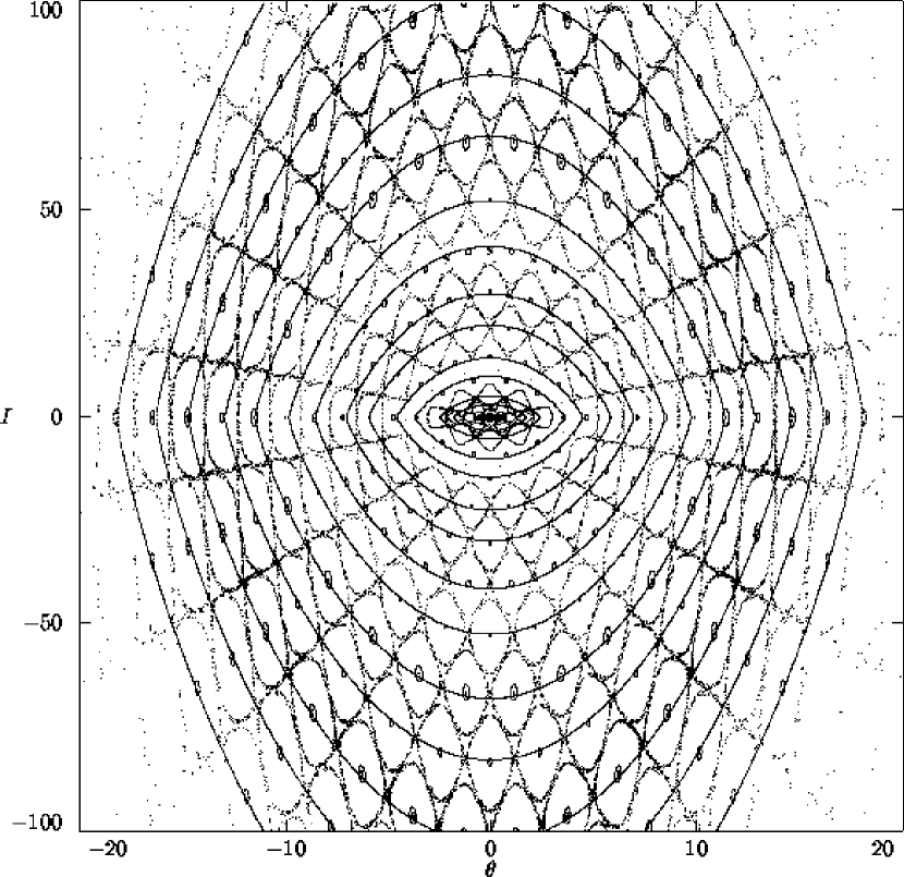
Figure 7: The resonant tori $J_{\pi}$ that are predicted by (48) for $n=1,m=1\ldots 15$. The web determined by the map (36) is superposed on top, along with one orbit near the center of each of the major islands. The predicted tori pass through the periodic points in the largest chains of islands outlined by the web.

4 Convex potentials ($\alpha<0$)

The maps with $m=2$, $\epsilon=0.3$ and $\alpha=-0.25$, $-0.5$, and $-0.75$ are shown in Figure 8a,b,c. These show the usual loop and box-like orbits, as well as a chaotic zone arising from a single orbit. Panel (d) shows the SOS for orbits integrated in the potential (27) with $\alpha=-0.5$, $c=0.05$, which shows good qualitative agreement with the map in panel (b). Note that the stochastic web seen near $\alpha=0$ develops into a stochastic sea by $\alpha=-0.75$.

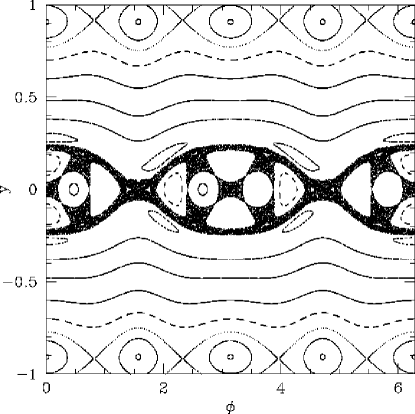
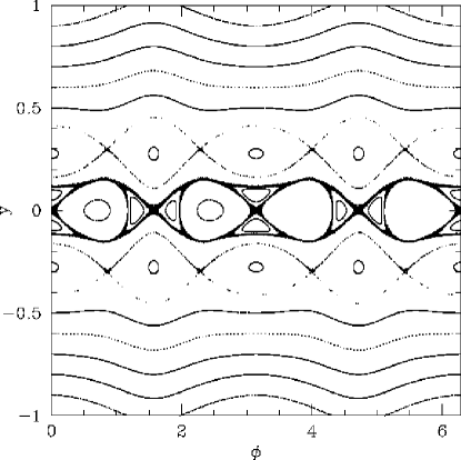
                                $(a)$ $(b)$

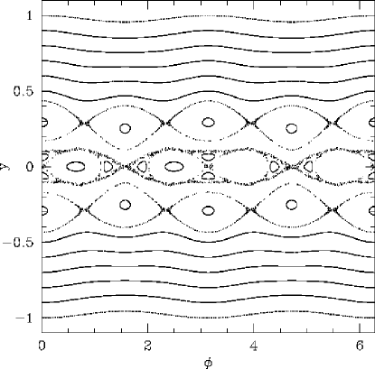
                                $(c)$ $(d)$

Figure 8: The map (15–17) with parameters $m=2$, $\epsilon=0.3$, and (a) $\alpha=-0.25$; (b) $\alpha=-0.5$; (c) $\alpha=-0.75$. The orbits have been iterated 1000 times, except for the chaotic orbits, which are iterated 5000 times to provide better coverage. (d) SOS for orbits in the potential (27), with $\alpha=-0.5$ and $c=0.05$. Each orbit is plotted for 1000 periods, except for the chaotic orbit, which is plotted for 10000 periods.

5 Other potentials

5.1 $m=1$

We can use the map to explore the behaviour of orbits in lopsided ($m=1$) potentials. In so doing we restrict ourselves to the range $\alpha\leq 1$ because dipole potentials with $1<\alpha\leq 2$ cannot be generated by a plausible density distribution (cf. eq. 23). The maps with $m=1$, $\epsilon=0.5$ and $\alpha=1$, $0.5$, $0$, and $-0.5$ are shown in Figure 9a,b,c,d. These show the usual loop orbits, box-like orbits, and chaotic orbits.

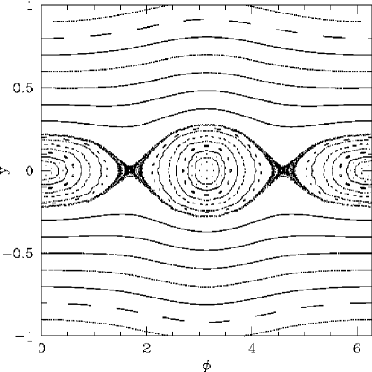
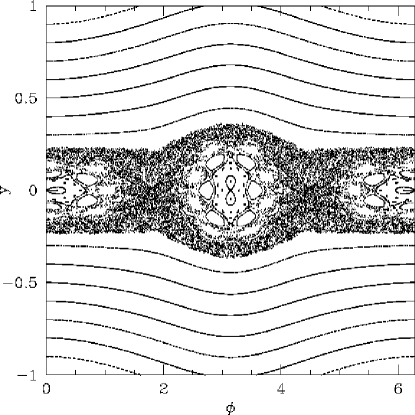
                                $(a)$ $(b)$

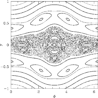
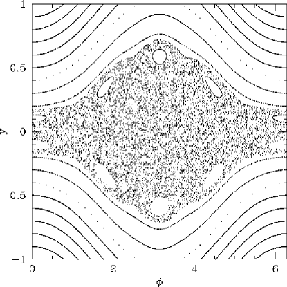
                                $(c)$ $(d)$

Figure 9: The map (15–17) with parameters $m=1$, $\epsilon=0.5$, and (a) $\alpha=1$; (b) $\alpha=0.5$; (c) $\alpha=0$, (d) $\alpha=-0.5$. The orbits have been iterated 1000 times, except for the chaotic orbits, which are iterated up to 20000 times to provide better coverage. The range $1<\alpha\leq 2$ is not examined because dipole potentials with this radial exponent cannot be generated by a scale-free density distribution (cf. eq. 23).

The maps provide preliminary estimates of which orbits are needed to construct self-consistent lopsided galaxies. The torques described by equation (15) are generated by a density distribution that is elongated along the axis $\phi=0$. When $\alpha=1$ (panel [a]) the loop orbits are most elongated (smallest $|y|$) when their apocenters are near $\phi=1.8,4.6$ and the box-like orbits have approximate $m=2$ symmetry around $\phi\simeq 0,\pi$; hence neither orbit family is likely to support a lopsided density distribution. The situation is more promising for $\alpha\leq 0$ (panels [c] and [d]). Here both the loop orbits and the chaotic sea are most elongated at $\phi=0$. Thus it may be possible to construct self-consistent lopsided galaxies with centrally concentrated density distributions.

5.2 Potentials that are not scale-free

In writing the precession rate as $g(\alpha,y)$ (eq. 7), we have assumed that the underlying axisymmetric potential is scale-free. More generally the precession rate is a function of the energy of the orbit in the underlying axisymmetric potential, $g(y,E)$, where $E={\textstyle{1\over 2}}v^{2}+\Phi(r)$ is assumed to be conserved since the non-axisymmetric component of the potential is small. Apart from the energy-dependent precession rate the map would remain unchanged.

5.3 Rotating potentials

The map can also be used to study orbits in rotating potentials. Let us suppose that the non-axisymmetric component of the potential is stationary in a frame rotating with pattern speed $\Omega_{p}$, that the potential has $m$-fold symmetry and that its azimuthal minimum lies along the ray $\phi=\Omega_{p}t$. The azimuthal angle in the rotating frame may be written $\psi\equiv\phi-\Omega_{p}t$. Then if $T_{r}(y,E)$ is the radial period of the particle orbit in the underlying axisymmetric potential, the map (15)–(17) is easily generalized to

$$y_{n}^{\prime} = y_{n}-{\textstyle{1\over 2}}\epsilon\sin m\psi_{n},$$

$$\psi_{n+1} = \psi_{n}+g(y_{n}^{\prime},E)-\Omega_{p}T_{r}(y_{n}^{\prime},E),$$

$$y_{n+1} = y_{n}^{\prime}-{\textstyle{1\over 2}}\epsilon\sin m\psi_{n+1}.$$ (49)

Note that $g$ is an odd function of $y$ while $T_{r}$ is even.

5.4 Three dimensions

We derive a mapping for motion in the three-dimensional generalization of the potential (24):

$$\Phi_{\alpha}({\bf r})=\left\{\begin{array}[]{cc}\hbox{sgn}(\alpha)\left(x_{1}^{2}+{\textstyle x_{2}^{2}\over\textstyle b^{2}}+{\textstyle x_{3}^{2}\over\textstyle c^{2}}\right)^{{\textstyle{1\over 2}}\alpha},&\alpha\not=0,\\ {\textstyle{1\over 2}}\log\left(x_{1}^{2}+{\textstyle x_{2}^{2}\over\textstyle b^{2}}+{\textstyle x_{3}^{2}\over\textstyle c^{2}}\right),&\alpha=0.\end{array}\right.$$ (50)

Here an orbit is defined by its vector angular momentum ${\bf L}$ and the unit direction vector of its apocenter, ${\bf n}$, where ${\bf L}\cdot{\bf n}=0$. We again prefer to deal with the dimensionless angular momentum, so we define ${\bf Y}={\bf L}/L_{c}(E)$. The torque gives a kick to the angular momentum vector which is concentrated at apocenter and equal to $-Q_{\alpha}{{\bf n}}_{n}\times{{\bf t}}_{n}$ where ${{\bf t}}=(n_{x},n_{y}/b^{2},n_{z}/c^{2})$. For nearly spherical potentials, $Q_{\alpha}$ is specified in (26). This kick is followed by a rotation of ${\bf n}$ about the updated ${\bf Y}$. Putting it all together,

$${{\bf Y}}_{n}^{\prime} = {{\bf Y}}_{n}-{\textstyle{1\over 2}}Q_{\alpha}{{\bf n}}_{n}\times{{\bf t}}_{n},$$

$${{\bf n}}_{n+1} = {\cal R}\big{(}{{\bf Y}}_{n}^{\prime},g(\alpha,|{{\bf Y}}_{n}^{\prime}|)\big{)}\,{{\bf n}}_{n}=-\frac{g(\alpha,|{\bf Y}_{n}^{\prime}|)}{|{\bf Y}_{n}^{\prime}|}{\bf n}_{n}\times{\bf Y}_{n}^{\prime},$$

$${{\bf Y}}_{n+1} = {{\bf Y}}_{n}^{\prime}-{\textstyle{1\over 2}}Q_{\alpha}{{\bf n}}_{n+1}\times{{\bf t}}_{n+1},$$ (51)

where ${\cal R}({\bf v},\theta)$ is a rotation about axis ${\bf v}$ by an angle $\theta$.

The mapping is apparently six-dimensional. However, it preserves the unit magnitude of ${\bf n}$ and the orthogonality of ${\bf Y}$ and ${\bf n}$. These two constraints on the motion reduce the dimension to four. Also, the mapping is symplectic. The proof is deferred to Appendix B.

A useful approximate description of the motion, valid when the potential is not far from spherical, is obtained by replacing the mapping equations (51) by the analogous differential equations

$${d{\bf Y}\over dn} = -Q_{\alpha}{{\bf n}}\times{{\bf t}},$$

$${d{\bf n}\over dn} = -\frac{g(\alpha,|{\bf Y}|)}{|{\bf Y}|}{\bf n}\times{\bf Y},$$ (52)

where $n$ is the orbit number. These have the integral of motion (cf. eq. B1)

$$\overline{H}({\bf Y},{\bf n})=\int^{y}g(\alpha,y)dy+{\textstyle{1\over 2}}Q_{\alpha}{\bf n}\cdot{\bf t}.$$ (53)

where $y=|{\bf Y}|$ and $\overline{H}$ is an averaged Hamiltonian analogous to equation (32). This integral can be used to solve for $y$ in terms of ${\bf n}$, so the equations of motion (52) can be replaced by equations for the two perpendicular unit vectors ${\bf n}$ and $\hat{\bf y}={\bf Y}/y$:

$${d\hat{\bf y}\over dn} = {Q_{\alpha}\over y}\left[{\bf t}\times{\bf n}-\hat{\bf y}\hat{\bf y}\cdot({\bf t}\times{\bf n})\right],$$

$${d{\bf n}\over dn} = -g(\alpha,y){\bf n}\times\hat{\bf y}.$$ (54)

The solutions of these equations of motion can be investigated using a surface of section (for example, defined by ${\bf n}\cdot\hat{\bf e}_{2}=0$), but we shall not do so in this paper.

6 Discussion

Our map provides a heuristic tool for studying the behaviour of eccentric orbits in non-spherical potentials. The map reproduces most of the qualitative features of orbits in non-axisymmetric potentials similar to those found in realistic galaxy models (e.g. Fig. 2). The map can be applied to a variety of potentials, as outlined in §5. In a limited sense, the map is more general than orbit integrations, since it does not depend on the specific radial form of the non-axisymmetric potential so long as the torque is concentrated near apocenter. The map is faster than direct numerical integration by 2–3 orders of magnitude—even more for near-radial orbits in centrally concentrated density distributions, which are difficult to integrate accurately. The speedup offered by the map is particularly important when exploring the long-term evolution of orbits in the central regions of galaxies: at 10 pc from the center of a typical giant galaxy the crossing time is only $10^{-5}$ of the Hubble time.

The map offers a powerful approach to studying many aspects of the behaviour of orbits in triaxial potentials, including the distribution of Liapunov times in chaotic orbits, the rate of mixing of a non-random distribution of stars, trapping of chaotic orbits, and the long-term influence of a central black hole on centrophilic orbits (Merritt 1996, Merritt & Fridman 1996, Merritt & Valluri 1996).

It may also be instructive to use the map to study the equilibrium and stability of approximate stellar systems, in which the torque between two elongated orbits is determined by the relative orientation of their apocenters. A very similar approximation has been used as the basis of heuristic explanations of bar formation in disk galaxies (Lynden-Bell 1979) and the radial-orbit instability in spherical galaxies (Palmer & Papaloizou 1987).

Appendix A Power series for the precession rate in power-law potentials

The goal of this Appendix is to provide a power-series expansion for the precession rate $g(\alpha,y)$ (eq. 7). For the sake of brevity we focus first on potentials with $\alpha>0$ (cf. eq. 1), extending the results to $\alpha\leq 0$ at the end.

We first extend the domain of $g$ by defining $g(\alpha,y)=0$ for $y>1$. We then take the Mellin transform

$$G(\alpha,s)\equiv\int_{0}^{\infty}g(\alpha,y)y^{s-1}dy;$$ (A1)

upon evaluating the integrals we have

$$G(\alpha,s)={\pi^{1/2}2^{s/2}\over\alpha h^{s}(\alpha)}{\Gamma({\textstyle{1\over 2}}+{\textstyle{1\over 2}}s)\Gamma(s/\alpha)\over\Gamma(1+{\textstyle{1\over 2}}s+s/\alpha)},\qquad\alpha>0,$$ (A2)

which holds in the right half-plane Re$(s)>0$.

The inverse Mellin transform is

$$g(\alpha,y)={1\over 2\pi i}\int_{\sigma-i\infty}^{\sigma+i\infty}G(\alpha,s)y^{-s}ds,$$ (A3)

where $\sigma$ is real and positive. For $0<y<1$, the integration contour can be closed by a semi-circle in the negative half-plane from $\sigma+i\infty$ to $\sigma-i\infty$. Since $1/\Gamma(z)$ is entire, the only contributions to the contour integral (A3) arise from poles in the functions $\Gamma(z)$ in the numerators of equations (A2), which occur at $z=-n$, $n=0,1,2,\ldots$ and have residues $(-1)^{n}/\Gamma(n+1)$. Thus

$$g(\alpha,y) = \pi^{1/2}\sum_{n=0}^{\infty}{(-1)^{n}h^{2n+1}(\alpha)\Gamma[-(2n+1)/\alpha]\over 2^{n-1/2}\alpha\Gamma[{\textstyle{1\over 2}}-n-(2n+1)/\alpha]\Gamma(n+1)}y^{2n+1}$$ (A4)

$$+\pi^{1/2}\sum_{n=0}^{\infty}{(-1)^{n}h^{\alpha n}(\alpha)\Gamma[(1-\alpha n)/2]\over 2^{\alpha n/2}\Gamma(1-n-\alpha n/2)\Gamma(n+1)}y^{\alpha n}.$$

Using the identity $\Gamma(z)\Gamma(1-z)=\pi/\sin\pi z$ this expression can be rewritten as

$$g(\alpha,y) = \pi-\pi^{1/2}\sum_{n=0}^{\infty}{h^{2n+1}(\alpha)\cot[\pi(2n+1)/\alpha]\Gamma[{\textstyle{1\over 2}}+n+(2n+1)/\alpha]\over 2^{n-1/2}\alpha\Gamma[1+(2n+1)/\alpha]\Gamma(n+1)}y^{2n+1}$$ (A5)

$$+\pi^{1/2}\sum_{n=1}^{\infty}{h^{\alpha n}(\alpha)\tan({\textstyle{1\over 2}}\pi\alpha n)\Gamma[n(1+\alpha/2)]\over 2^{\alpha n/2}\Gamma[(1+\alpha n)/2]\Gamma(n+1)}y^{\alpha n},\qquad\alpha>0.$$

In the limit $y\to 0$ we recover equations (9) and (10).

For $\alpha<0$ we can apply the relation (14) to obtain

$$g(\alpha,y) = {2\pi\over 2-\beta}+\pi^{1/2}\sum_{n=0}^{\infty}{h^{2n+1}[2\beta/(2-\beta)]\tan[\pi(2n+1)/\beta]\Gamma[(2n+1)/\beta]\over 2^{n-1/2}\beta\Gamma[{\textstyle{1\over 2}}-n+(2n+1)/\beta]\Gamma(n+1)}y^{2n+1}$$ (A6)

$$+\pi^{1/2}\sum_{n=1}^{\infty}{h^{2\beta n/(2-\beta)}[2\beta/(2-\beta)]\tan[\pi\beta n/(2-\beta)]\Gamma[2n/(2-\beta)]\over 2^{\beta n/(2-\beta)-1}(2-\beta)\Gamma[{\textstyle{1\over 2}}+\beta n/(2-\beta)]\Gamma(n+1)}y^{2\beta n/(2-\beta)},$$

where $\beta=-\alpha$, $\alpha<0$. The series (A5) and (A6) are asymptotic: if truncated after a fixed number of terms the series become arbitrarily accurate as $y\to 0$, but for fixed $y$ the series do not generally converge as more terms are added.

Appendix B The three-dimensional mapping is symplectic

We claim that the generalization of the two-dimensional mapping (eqs. 15–17) to triaxial potentials (eqs. 51) is symplectic. There are two routes to the proof: one familiar but messy, the other less familiar but more elegant and illuminating. We outline the first and describe the second in detail. On the messy road, we define two pairs of canonically conjugate variables. One pair joins the magnitude of the angular momentum and the argument of apocentre and the other the $x_{3}$-component of the angular momentum vector and the longitude of the ascending node on the $x_{1}$-$x_{2}$ plane. That these coordinates are canonically conjugate is a basic result of classical celestial mechanics (e.g. Plummer 1960). Then we express the map in terms of these coordinates, derive the Jacobian ${\bf M}$ of the mapping transformation, and show after some algebraic labor, that this Jacobian fulfills the requirements that a canonical transformation must satisfy, namely: ${\bf M}^{T}{\bf J}{\bf M}={\bf J}$, where ${\bf J}$ is the $4\times 4$ canonical symplectic matrix (see Goldstein 1980 for definitions and details).

We prefer to observe that the mapping derives from the Hamiltonian:

$$H=H_{y}({\bf Y})+{\delta}_{1}(t)H_{n}({\bf n}),$$ (B1)

where $H_{y}=\int^{y}g(\alpha,y)dy$, $y=|{\bf Y}|$, and $H_{n}={\textstyle{1\over 2}}Q_{\alpha}{\bf n}\cdot{\bf t}$, with the help of the bracket:

$$\{F_{1}({\bf Y},{\bf n}),F_{2}({\bf Y},{\bf n})\}={\bf Y}\cdot({\mbox{\boldmath$\nabla$}}_{{\bf Y}}F_{1}\times{\mbox{\boldmath$\nabla$}}_{{\bf Y}}F_{2})+{\bf n}\cdot({\mbox{\boldmath$\nabla$}}_{{\bf n}}F_{1}\times{\mbox{\boldmath$\nabla$}}_{{\bf Y}}F_{2}+{\mbox{\boldmath$\nabla$}}_{{\bf Y}}F_{1}\times{\mbox{\boldmath$\nabla$}}_{{\bf n}}F_{2}).$$ (B2)

The bracket gives the time evolution of any real valued function $F_{1}$ of these two vectors, along the vector field generated by another such function $F_{2}$, through the relation

$${d\over dt}F_{1}({\bf Y},{\bf n})=\{F_{1},F_{2}\}.$$ (B3)

The equations for the time evolution of ${\bf Y}$ and ${\bf n}$ along the vector field generated by $H_{y}$ are:

$$\frac{d}{dt}{\bf Y} = 0,$$

$$\frac{d}{dt}{\bf n} = -\frac{g(\alpha,|{\bf Y}|)}{|{\bf Y}|}{\bf n}\times{\bf Y}.$$ (B4)

The first of these equations states that ${\bf Y}$ is conserved by $H_{y}$. The second is telling us $H_{y}$ causes a rotation of ${\bf n}$ by angle $g$ about vector ${\bf Y}$. This is one of the mapping steps. $H_{n}$ on the other hand generates motion:

$$\frac{d}{dt}{\bf Y} = -Q_{\alpha}{\bf n}\times{\bf t},$$

$$\frac{d}{dt}{\bf n} = 0.$$ (B5)

When we compose the action of $H_{y}$ and $H_{n}$, in the manner dictated by the periodic delta function, we recover the mapping (51). Now we still have to show that the dynamics generated by this bracket is canonical. The bracket is known as a Lie-Poisson bracket and is closely related to the bracket used in the study of conservative rigid body dynamics (see Marsden 1992 for a general discussion, and Touma and Wisdom 1994 for a discussion of Lie-Poisson brackets in an astronomical context). On a suitably defined pair of canonical variables, the bracket reduces to the canonical Poisson bracket and the dynamics generated by the bracket consists of canonical transformations. Thus, $H_{y}$ and $H_{n}$ separately generate symplectic mappings and their composition via the mapping is therefore symplectic, completing our proof.

References

- Binney (1982) Binney, J. 1982, MNRAS 201, 1
- Binney & Spergel (1982) Binney, J., & Spergel, D. 1982, ApJ 252, 308
- Binney & Tremaine (1987) Binney, J. J., & Tremaine, S. 1987, Galactic Dynamics (Princeton: Princeton University Press)
- de Zeeuw (1985) de Zeeuw, T. 1985, MNRAS 216, 273
- Gebhardt et al. (1996) Gebhardt, K., Richstone, D., Ajhar, E. A., Lauer, T. R., Byun, Y.-I., Kormendy, J., Dressler, A., Faber, S. M., Grillmair, C., and Tremaine, S. 1996, AJ 112, 105
- Gerhard & Binney (1985) Gerhard, O. E., & Binney, J. 1985, MNRAS 216, 467
- Goldstein (1980) Goldstein, H., 1980, Classical Mechanics, 2nd ed. (Reading: Addison-Wesley)
- Grant & Rosner (1994) Grant, A. K., & Rosner, J. L. 1994, Am. J. Phys. 62, 310
- Kormendy & Richstone (1995) Kormendy, J., & Richstone, D. 1995, ARAA 33, 581
- Kuijken (1993) Kuijken, K. 1993, ApJ 409, 68
- Lees & Schwarzschild (1992) Lees, J. F., & Schwarzschild, M. 1992, ApJ 384, 491
- Lichtenberg & Lieberman (1992) Lichtenberg, A. J., & Lieberman, M. A., 1992, Regular and Chaotic Dynamics, 2nd ed. (Springer, New York)
- Lynden-Bell (1962) Lynden-Bell, D. 1962, MNRAS 124, 95
- Lynden-Bell (1979) Lynden-Bell, D. 1979, MNRAS 187, 101
- Marsden (1992) Marsden, J. E. 1992, Lectures on Mechanics (Cambridge: Cambridge University Press)
- Merritt (1996) Merritt, D. 1996, Science 271, 337
- Merritt & Fridman (1996) Merritt, D., & Fridman, T. 1996, ApJ 460, 136
- Merritt & Valluri (1996) Merritt, D., & Valluri, M. 1996, ApJ 471, 82
- Miralda-Escudé & Schwarzschild (1989) Miralda-Escudé, J., & Schwarzschild, M. 1989, ApJ 339, 752
- Palmer & Papaloizou (1987) Palmer, P. L., & Papaloizou, J. 1987, MNRAS 224, 1043
- Pfenniger & de Zeeuw (1989) Pfenniger, D., & de Zeeuw, T. 1989, in Dynamics of Dense Stellar Systems, ed. D. Merritt (Cambridge: Cambridge University Press), 81
- Plummer (1960) Plummer, H. C. 1960, An Introductory Treatise on Dynamical Astronomy (New York: Dover)
- Richstone (1980) Richstone, D. O. 1980, ApJ 238, 103
- Richstone (1982) Richstone, D. O. 1982, ApJ 252, 496
- Schwarzschild (1979) Schwarzschild, M. 1979, ApJ 232, 236
- Schwarzschild (1993) Schwarzschild, M. 1993, ApJ 409, 563
- Sridhar & Touma (1997) Sridhar, S., & Touma, J. 1997, MNRAS 287, L1
- Touma & Wisdom (1994) Touma, J., & Wisdom, J. 1994, AJ 107, 1189
- Whittaker (1959) Whittaker, E. T. 1959, A Treatise on the Analytical Dynamics of Particles and Rigid Bodies, 4th ed. (Cambridge: Cambridge University Press)