Updated Solar Models

Abstract

Solar models computed with mass loss, microscopic diffusion of helium and heavy element, and with updated physics have been evolved from the pre-main sequence to present day; they are compared to the observational constraints including lithium depletion and to the seismic reference model of Basu et al. ([1996]), derived by inversion. Microscopic diffusion significantly improves the agreement with the observed solar frequencies and agree with the seismic reference model within $\pm 0.2\%$ for the sound velocity and $\pm 1\%$ for the density, but slightly worsens the neutrino problem. Neither microscopic diffusion nor overshooting explain the observed lithium depletion consistently with helioseismological constraints, while a mass loss process does it. Models computed with OPAL equation of state and opacities are in a better agreement with the seismic sound speed. To reach the level of precision of helioseismological observations the accuracy of solar models still needs to be improved by one magnitude; any such improvement will necessitate equation of state and opacity data taking into account of detailed changes in the mixture.

1 Introduction

The successful development of helioseismology imposes very strong constraints on the structure of the interior of solar models and has led solar modelers to improve the physical inputs of their models. One important step is the insertion of microscopic diffusion. The solar models with microscopic diffusion (Proffitt & Michaud [1991]; Bahcall & Pinsonneault [1992]; Christensen-Dalsgaard et al. [1993]; Kovetz & Shaviv [1994]; Proffitt [1994]; Morel et al. [1996]; Gabriel & Carlier [1997]; Degl’Innocenti et al. [1997]; Brun et al. [1997]) closely agree with constraints of the solar interior inferred by helioseismology as reviewed by Christensen-Dalsgaard et al. ([1996]). The recent improvements of equation of state (Rogers et al. [1996]) and opacities (Iglesias & Rogers [1996]) have brought the difference between the solar sound speed of the seismic model of Basu et al. ([1996]), from LowL data (hereafter, ”seismic reference model”) and the sound speeds computed from present day solar models within a rms discrepancy better than 0.2% (Gough et al. [1996]); the values of the radius at the bottom of the convection zone (Christensen-Dalsgaard et al. [1991]) and the helium abundance at the solar surface (Pérez Hernández & Christensen-Dalsgaard [1994]; Antia & Basu [1994]; Basu & Antia [1995]) predicted by models agree within the error bar with their values inferred from helioseismology (e.g., Basu [1997]). Nevertheless the large excesses of neutrino rates (e.g., Bahcall [1997]) and of lithium abundance predicted by the models still appear in strong conflict with the good agreement between the structure of the model and the inferred sound speed and density. Up to now, all attempts to mix the Sun in such a way as to minimize the discrepancies between solar observations and predictions for, either neutrinos or lithium depletion, are ruled out by helioseismology. So mixing may be not the relevant process; it appears thus that for the neutrino problem the discrepancies are in pass to be understood rather through a modest extension of the electroweak theory (Bahcall & Krastev 1996) than through improvements or change of physics. Promising processes for accounting for the observed lithium depletion are mass loss (Boothroyd et al. [1992]; Guzik & Cox [1995]; Henyey & Ulrich [1995]) and turbulent diffusion induced by rotation (Charbonnel et al. [1992], Chaboyer et al. [1995], Richard et al. [1996]).

In this work, we have reconsidered the effect of microscopic diffusion and discussed the estimation of the heavy element content used in opacities calculations. Starting from chemically homogeneous pre-main sequence models we have computed calibrated solar models with and without microscopic diffusion. We have considered two different mass loss laws, undershooting and overshooting of convection zones, and also examined the effects of different equation of state and opacities. However turbulent diffusion induced either by rotation or internal waves (Schatzman [1993], Montalban & Schatzman [1996]) is ignored.

The models have been compared to the seismic reference model through the quantities $(c_{\odot}-c_{\rm model})/c_{\odot}$ and $(\rho_{\odot}-\rho_{\rm model})/\rho_{\odot}$, $c_{\rm model}$, $c_{\odot}$, $\rho_{\rm model}$ and $\rho_{\odot}$ are, respectively, the sound speeds and the densities of the model and of the seismic reference model. The oscillation frequencies of the solar models have been compared to the GONG data observations. Likewise, the neutrino fluxes expected for the three experiments and the lithium depletion at present age have been computed and compared with the measurements. These solar models are updated and improved versions of the models discussed in Berthomieu et al. ([1993]).

In Section 2 global parameters and helioseismological constraints are briefly recalled for references and notations. In Section 3 the physics is described. Outlines of numerical techniques used so far are given in Section 4. Results and discussion are presented in Section 5 and the conclusions in Section 6. Two appendices are devoted to detailed discussions of heavy element abundances which enter in equation of state and opacities.

2 Observational constraints and calibration of solar models

For reference, the solar global parameters, at present, and the constraints inferred from helioseismology are given in Table 1 were the standard notations and the units are recalled in the caption. Recent observed neutrino fluxes at earth from the Gallium $\Phi_{\rm Ga}$, Chlorine $\Phi_{\rm Cl}$ and Kamiokande $\Phi_{\rm Ka}$ experiments are reported. The frequency differences $\overline{\delta\nu}_{02}$ and $\overline{\delta\nu}_{13}$ which correspond to mean values of recent observations from the ground based networks IRIS and BiSON and from the spatial experiments VIRGO and GOLF are given (see section 4.2). There $Y_{\odot}$ is the surface abundance per unit mass of helium, determined by Basu & Antia (1995) with respectively MHD and OPAL equation of state, and $R_{\rm ZC}$ is the radius at the bottom of the convection zone. The solar age given in Table 1 corresponds to the start of main sequence evolution. We have adopted an evolutionary time of 4.5 Gyr for models starting from the zero-age main sequence and 4.55 Gyr for models including pre-main sequence.

Table 1: Solar data at present day; the units are, $10^{33}$ g for the mass $M_{\odot}$, $10^{10}$ cm for the radius $R_{\odot}$, $10^{33}$ erg s^-1 for the luminosity $L_{\odot}$, Gyr for the age $t_{\odot}$, dex (¹H=12) for the surface depletion of lithium Li_⊙, SNU for $\Phi_{\rm Ga}$ and $\Phi_{\rm Cl}$, ev day^-1 for $\Phi_{\rm Ka}$, $\mu$Hz for the frequency differences $\overline{\delta\nu}_{02}$ and $\overline{\delta\nu}_{13}$.

$M_{\odot}$	$1.9891\pm 0.0004$	Cohen & Taylor ([1968])
$R_{\odot}$	$6.9599\pm 0.001$	Guenther et al. ([1992])
$L_{\odot}$	$3.846\pm 0.005$	Guenther et al. ([1992])
$t_{\odot}$	$4.52\pm 0.4$	Guenther et al. ([1992])
$(Z/X)_{\odot}$	$0.0245\times(1\pm 0.1)$	Grevesse & Noels ([1993])
$Y_{\odot}$	0.246 ; 0.249	Basu & Antia (1995)
$R_{\rm ZC}/R_{\odot}$	$0.713\pm 0.003$	Christensen-Dalsgaard
		et al. ([1991])
Li⊙	$1.16\pm 0.1$	Anders & Grevesse ([1989])
$\Phi_{\rm Ga}$	$69^{+7.8}_{-8.1}$	Hampel et al. ([1996])
$\Phi_{\rm Cl}$	$2.55\pm 0.23$	Davis ([1993])
$\Phi_{\rm Ka}$	$0.29\pm 0.02$	Fukuda et al. ([1996])
$\overline{\delta\nu}_{02}$	$9.01\pm 0.05$	Provost ([1997])
$\overline{\delta\nu}_{13}$	$15.90\pm 0.08$	Provost ([1997])

The amount of heavy element per unit of mass for present day $Z_{\odot}=0.0181(1\pm 0.1)$ is derived from $Y_{\odot}$ and from $(Z/X)_{\odot}$ the ratio of heavy element to hydrogen measured at the surface.

The solar models discussed in this paper are calibrated within a relative accuracy better than $10^{-4}$ by adjusting: i) the ratio $l/H_{\rm p}$ of the mixing-length to the pressure scale height, ii) the protosolar mass fraction $X_{\rm p}$ of hydrogen, iii) the protosolar mass fraction $(Z/X)_{\rm p}$ of heavy element to hydrogen and, iv) the mass $M_{\rm p}$ of the primitive Sun, in order that, at present day, the models have the values of Table 1 for, i) the luminosity, ii) the radius, iii) the mass fraction of heavy element to hydrogen and, iv) the solar mass.

3 Physics of Solar models

3.1 Initial conditions and nuclear network

Here the evolution of solar models, but one, include the pre-main sequence; they are initialized with chemically homogeneous models, according to the procedure of Iben ([1975]) using a fixed contraction factor $c\equiv 0.02L_{\odot}M_{\odot}^{-1}K$, see details in Morel ([1997]).

The general nuclear network we used contains the following twelve species ¹H, ²H, ³He, ⁴He, ⁷Li, ⁷Be, ¹²C, ¹³C, ¹⁴N, ¹⁵N, ¹⁶O and ¹⁷O which enter into the most important nuclear reactions of the PP+CNO cycles. The relevant nuclear reaction rates are taken from the tabulations of Caughlan and Fowler ([1988]). Weak screening is assumed. The abundance of any chemical is explicitly computed i.e., no element is assumed to be at equilibrium. The protosolar abundances of deuterium and of species heavier than helium are calculated using their nuclide ratios with respect to hydrogen (Anders & Grevesse [1989]); the protosolar mass fraction $Y_{\rm p}$ of helium is taken as: $Y_{\rm p}\equiv 1-X_{\rm p}(1+(Z/X)_{\rm p})$; the protosolar ³He abundance is derived from the protosolar ${}^{4}{\rm He}\equiv Y_{\rm p}$ abundance according to the isotopic ratio ${}^{3}{\rm He}/^{4}{\rm He}=1.42\times 10^{-4}$. For lithium, we have used the ratio by number $(^{7}{\rm Li}/^{1}{\rm H})_{\rm p}=3.277$ dex; the unknown protosolar ratio by number ⁷Be/¹H is taken to $-3.58$ dex i.e., about its equilibrium value at center of the Sun. As a definition, we have considered that a pre-main sequence model becomes a main sequence model as soon as 99% of the energy released is from nuclear; this transition occurs at an age between 40 Myr and 80 Myr. At that time, due to the CNO nuclear energy produced by the conversion of protosolar ¹²C onto ¹⁴N, the models have a convective core of typical extent $\sim 10\%$ of the total radius and the outer solar convection zone has already receded about to its present day location. We emphasize the importance of pre-main sequence evolution for the study of the depletion of light element; with physical conditions of solar homogeneous zero-age main sequence and with the nuclide abundances of ²H and ⁷Li, the two reactions ²H($p,\gamma)\,^{3}$He and ⁷Li($p,\alpha)\,^{4}$He are strongly far from equilibrium; a homogeneous zero-age main sequence model can be found only if the abundances of ²H and ⁷Li are taken near to their equilibrium values, that is inappropriate for studies of light element depletion.

3.2 The opacities and equation of state

We have used the opacities of Livermore Library (Rogers & Iglesias [1992]; Rogers et al. [1996]) extended with the low temperature opacities of Kurucz’s ([1991]) interpolated with a birational spline interpolation (Houdek & Rogl [1996]) and, either the CEFF equation of state (Christensen-Dalsgaard & Däppen [1992]), or the OPAL equation of state (Rogers et al. [1996]). Because it depends not much on $Z$ and to avoid too heavy numerical computations, we have fixed the amount of heavy element in the equation of state to values closed to their mean amounts in calibrated models namely, $Z\equiv 0.0175$ for solar models without microscopic diffusion and $Z\equiv 0.0190$ for solar models with microscopic diffusion. The opacities and equation of state are tabulated for mixtures with various amounts of hydrogen, $X_{{}^{1}{\rm H}}$, but with fixed ratios between the species of heavy element. During the evolution these ratios are modified by the thermonuclear reactions and by the microscopic diffusion and the new mass fraction of each isotope needs to be re-estimated as detailed in Appendix A. In main sequence solar models a local maximum of ³He occurs around $R\sim 0.3R_{\odot}$, it amounts to 10% of the local helium content $X_{{}^{3}{\rm He}}\sim 0.1\times X_{{}^{4}{\rm He}}\sim Z$, here $X_{{}^{3}{\rm He}}$ and $X_{{}^{4}{\rm He}}$ are the mass fractions of, respectively, ${}^{3}{\rm He}$ and ${}^{4}{\rm He}$; as seen in Appendix B this effect needs to be taken into account in the calculation of the amount of heavy element used for the determination of opacities and equation of state.

3.3 Diffusion

The turbulent diffusion is ignored in the solar models discussed in this paper. Various treatment of the microscopic microscopic diffusion leads to diffusion rates in good agreement (Bahcall & Pinsonneault [1995]). We have used the microscopic diffusion coefficients of Michaud & Proffitt ([1993]). All chemicals including either $X_{\rm nCNO}$ or $\cal X_{\rm Z}$ (see below), but ¹H and ⁴He, are trace elements. Equation (14) of Michaud & Proffitt valid for a H-He mixture, is approximatively extended to a mixture including heavier elements, by writing (Alecian [1995]):

$$X_{{}^{1}\rm H}V_{{}^{1}\rm H}=-(1-X_{{}^{1}\rm H}-Z)V_{{}^{4}\rm He}$$ (1)

instead of $X_{{}^{1}\rm H}V_{{}^{1}\rm H}=-(1-X_{{}^{1}\rm H})V_{{}^{4}\rm He}$, therefore $X_{{}^{1}\rm H}+X_{{}^{4}\rm He}+Z\equiv 1$ even with microscopic diffusion, here $V_{{}^{1}\rm H}$ and $V_{{}^{4}\rm He}$ are respectively the diffusion velocities of hydrogen and helium.

The opacities and equation of state are functions of the heavy element content $Z$, through the number of free electrons and the abundances of efficient absorbers which do not necessarily belong to the nuclear network e.g., ⁵⁶Fe. Due to diffusion and nuclear reactions, $Z$ changes as the Sun evolves, as well as the ratios between the abundances of chemicals; in the following we shall designate by $Z_{\kappa}$ the amount of heavy element used for the computation of opacities in models and we discuss next three approximate estimates employed here.

For the calculation of solar models without microscopic diffusion either, i) $Z_{\kappa}$ is given by Eq. (A) resulting of detailed calculations of abundances including the changes due to the nuclear reactions – as detailed in Appendix A – but, the ratios between the abundances are not consistent with the values used for the creations of equation of state and opacities data or, ii) $Z_{\kappa}$ is kept to its protosolar value $Z_{\kappa}=Cte=Z_{\rm p}$ i.e., one neglects the changes of abundances of heavy element.

For solar models with microscopic diffusion the alternative is more subtle, in the core it is expected that the abundances of the heaviest chemicals are magnified by gravitational settling with the consequence of an enhancement of the opacity there (Turck-Chièze et al. [1993]), therefore a careful estimate of $Z_{\kappa}$ is required to infer the effects of this process.

A first possibility is to consider that, since opacity tables are available only for one mixture of heavy element, we do not know how to take into account properly their changes due both to nuclear reactions and diffusion, so we just ignore them and take $Z_{\kappa}=Cte=Z_{\rm p}$.

A second possibility is to model the diffusion of heavy element as a whole, by means of a mean fictitious chemical ${\cal X}_{\rm Z}$, with the mean atomic weight $M_{\rm Z}$, and the mean charge $z_{\rm Z}$, of the heavy species; ${\cal X}_{\rm Z}$ being diffused as an extra trace element but it is not affected by the thermonuclear reactions; then the ratios between the heavy element entering onto ${\cal X}_{\rm Z}$ are fixed, their changes due to thermonuclear reactions are ignored and ${\cal X}_{\rm Z}$ can differ from its value given by Eq. (A).

We have also investigated a third possibility – labeled $\cal Z$ – namely, $Z_{\kappa}$ is separated in two parts, the first consists of the chemicals heavier than helium which, belonging to the CNO nuclear network, are both diffused and nuclearly processed, the second part consists of a fictitious mean non-CNO species $X_{\rm nCNO}$, of atomic weight $M_{\rm nCNO}$ and charge $z_{\rm nCNO}$, which is only diffused (Eq. (A)). Hence in the estimate of $Z_{\kappa}$, enter into account the changes of CNO abundances caused by diffusion, nuclear processes and the effects of the large gravitational settling of heaviest non-CNO species but, the ratios between the chemicals can differ from the values used for the computations of opacities and equation of state data. This third possibility is similar to the treatment of Proffitt ([1994]), where in addition, an attempt is made – namely its Eq. (3) – to approximate the changes of ratios between the heavy element in the calculation of $Z_{\kappa}$.

For the mean chemicals, ${\cal X}_{\rm Z}$ and $X_{\rm nCNO}$, we have only taken into account the heavy element with abundances larger than 7.0 in the table 2 of Anders & Grevesse (1989), namely: C, N, O, Ne, Mg, Si, Fe; we have found, for ${\cal X}_{\rm Z}$: $M_{\rm Z}=17$, $z_{\rm Z}=8$ and, for $X_{\rm nCNO}$: $M_{\rm nCNO}=27$ and $z_{\rm nCNO}=13$.

3.4 Convection, overshooting and undershooting

The basic formulation of the standard mixing length theory is used. The convection zones are delimited according to the Schwarzschild’s criterion. In convection zones and in their extensions by overshooting or undershooting, the chemicals are simultaneously homogenized and integrated with respect to time (Morel & Schatzman [1996]; Morel [1997]). The mixing includes every convective zone and its extent by undershooting or overshooting where the temperature gradient is kept equal to its adiabatic value (Zahn [1991]). The amount of overshooting of a convective core is taken as $\zeta_{\rm ov}\min(H_{\rm p},R_{\rm cv})$, $\zeta_{\rm ov}$ is the overshooting factor and $R_{\rm cv}$ is the radius of the convective core; at the outer limit i.e., in the atmosphere, no overshooting is allowed. With an overshooting factor of $\zeta_{\rm ov}\sim 0.3$, the young Sun has a convective core, up to the age $t\sim 1\,$Gyr; this results an enrichment in nuclear fuel which does not lead to significant changes in the present day solar model (Morel et al. [1996]).

3.5 Lithium depletion and mass loss

The depletion of lithium is mainly caused by the reaction ⁷Li($p,\alpha)\,^{4}$He. For solar conditions ($T\la 1.5\times 10^{7}$K) it is, at least, 10 times more efficient than all the reactions involving ⁷Li, except ⁷Li($d,n)2\,^{4}$He which is only two times less efficient (Caughlan & Fowler [1988]), but the abundance of deuterium being almost zero, this reaction depletes no lithium. Therefore we can estimate that the abundance of ⁷Li resulting from our calculations is $\sim 2\%$ over-estimated – ⁶Li destroyed around $2\times 10^{6}$K is not observed in the solar photosphere (Böhm-Vitense [1992]).

Figure 1: Fractional differences for sound velocities (left) and densities (right) between the solar models without microscopic diffusion of Table 3 and the seismic reference model of Basu et al. ([1996]). The main features of the physics used in each model are schematically recalled with the notations of Table 2. S1 {CEFF, OPAL92, PMS} (thin full), S2 {CEFF, OPAL95, PMS} (thick full), S3 {OPAL, OPAL95, PMS} (thin dashed), S4 {OPAL, OPAL95, ZAMS} (thick dashed).

As suggested (Soderblom et al. [1993]) by the observations of the Pleiades (80-100 Myr) for stars with masses closer to the solar value only small lithium depletion seems to occur during the pre-main sequence while, from the observations of the Hyades (600 Myr) it appears that the most important amount of the depletion should occur during the first $\lse 500$ Myr of the main sequence. Such a depletion can result from mass loss: in a star of mass $M\sim 1.1M_{\odot}$, at the onset of main sequence the convection zone recedes at mass $m>1M_{\odot}$, the layers which correspond to the location of the present day convection zone i.e., $m\in[\sim 0.97M_{\odot},\sim 1M_{\odot}]$, are radiative and the temperature there is large enough to deplete the lithium. A mass loss of $\sim 0.1M_{\odot}$, occurring at that time ejects the outer layers, and the present day convection zone is formed by mixing these lithium poor shells, with the result of the observed enhancement of lithium depletion. Following Guzik & Cox ([1995]) we have studied two laws of mass loss rate namely, a mild mass loss rate:

$$\dot{M}=-2\times 10^{-10}\exp(-\frac{t}{0.45})\ M_{\odot}\ {\rm yr}^{-1},$$ (2)

and a strong mass loss rate:

$$\left\{\begin{array}[]{ccl}\dot{M}&=&-5\times 10^{-10}\ M_{\odot}\ {\rm yr}^{-1}\ {\rm if}\ M(t)>M_{\odot},\\ \dot{M}&=&0\ {\rm otherwise;}\end{array}\right.$$ (3)

here $t$, in Gyr, is the age of the model and $M(t)$ is its mass at time $t$; with the mild mass loss rate the protosolar mass $M_{\rm p}\sim 1.1M_{\odot}$ is adjusted to fit the present day solar mass.

4 Computation of models and frequencies

4.1 Solar models

The solar models discussed in this paper have been computed using the code CESAM (Morel [1997]); along the evolution atmospheres are restored (Morel et al. [1994]). The number of mass shells and the time steps are fixed according to numerical criteria; at the onset of calculations (pre-main sequence) the number of integration points is typically of the order of 550 and around 1030 for the present day solar models ($\sim 950$ for the core and the envelope, $\sim 80$ for the atmosphere); the whole evolution involved about 140 models, with 60 models from zero-age main sequence to present day. It has been checked that the numerical internal accuracy on sound speed is better than $5\times 10^{-4}$ for the whole model, but differences below that level are perhaps meaningless due to uncertainties of interpolated physical data. It is assumed that the lost mass is simply detached from the star by some process which is not described. We also emphasize on the fact that in our calculations, the ⁷Li depletion results from simultaneous computations of chemical changes due to nuclear reactions, diffusion and convective mixing. The estimated fluxes for the three neutrino experiments, $\Phi_{\rm Cl}$, $\Phi_{\rm Ga}$ and $\Phi_{\rm Ka}$ are computed according to Berthomieu et al. ([1993]).

4.2 p-Mode Oscillation Calculations

The frequencies of linear, adiabatic, global acoustic modes of the solar models have been computed for degrees $\ell$=0 to 150 and have been compared to the observations. For the computation of frequencies the models are extended to about 1800 shells. The characteristic low degree p mode frequency differences $\Delta\nu_{n,\ell}=\nu_{n,\ell}-\nu_{n-1,\ell+2}$ for $\ell$=0 and 1, which provide information on the properties of the core of the Sun, have been fitted by linear regressions with respect to $n$:

$$\Delta\nu_{n,\ell}=\delta\nu_{n,\ell}+S_{\ell}(n-n_{0}),$$

with $n_{0}=21$ and for $\ell=0,1$, both for the observations and the theoretical frequencies. The quantities $\overline{\delta\nu}_{02}$ and $\overline{\delta\nu}_{13}$ given in Table 1 are weighted mean values of the $\delta\nu_{n,\ell}$ derived from BiSON (Chaplin et al. [1997]), IRIS (Gelly et al. [1997]), GOLF (Grec et al. [1997]) and VIRGO (Fröhlich et al. [1997]). Despite the fact that solar activity is not expected to have a large influence on the solar core structure, we have also represented in Fig. 3 another mean restricted to low activity observations.

For the gravity modes which have not yet been observed, we give the characteristic asymptotic spacing period $P_{0}$ according to Provost & Berthomieu ([1986]).

5 Results and discussion

We have computed solar models without microscopic diffusion, (labeled ”S$n$”, $n=1,\ldots 4$) and solar models with microscopic diffusion (labeled ”D$n$”, $n=1,\ldots,12$) using the physics and physical data described Sect. 3 and summarized in Table 2 for each model.

Table 2: Summary of physical inputs for solar models with and without microscopic diffusion of Table 3 and Table 4. For each model the flag signals the physical option employed. In the first three lines, the evolutionary time is mentioned; the two next, indicate either, if the evolution includes the pre-main sequence and then the nuclear network with 12 species is used or, if the evolution is initialized from the homogeneous zero-age main sequence then it uses the simplified nuclear network with ²H, ⁷Li and ⁷Be at equilibrium. In the four next lines the flags indicate if overshoot (Ov-shoot), undershoot (Un-shoot), mild mass loss rate (mMLR) or strong mass loss rate (sMLR) are allowed for. In the next three lines is indicated how the amount of heavy element is computed for the calculation of opacities (see text). In the last lines the mass ratio of heavy element to hydrogen, used for the calibration, the opacities and the equation of state used are given.

	S1	S2	S3	S4	D1	D2	D3	D4	D5	D6	D7	D8	D9	D10	D11	D12
age 4.65 Gy												*	*
age 4.55 Gy	*	*	*		*	*	*	*	*	*	*			*	*	*
age 4.50 Gy				*
PMS 12 Chem.	*	*	*		*	*	*	*	*	*	*	*	*	*	*	*
ZAMS 9 Chem.				*
Ov-shoot											*
Un-shoot										*
mMLR									*
sMLR								*							*
$Z_{\kappa}=Z_{\rm p}=Cte$	*	*	*	*	*			*	*	*	*	*	*	*
$Z_{\kappa}$=$\cal Z$															*	*
$Z_{\kappa}={\cal X}_{\rm Z}$						*	*
$(Z/X)_{\odot}$=0.0245	*	*	*	*	*	*	*	*	*	*	*	*		*	*	*
$(Z/X)_{\odot}$=0.0260													*
opa-OPAL92	*
opa-OPAL95		*	*	*	*	*	*	*	*	*	*	*	*	*	*	*
EOS-CEFF	*	*			*	*		*	*	*	*	*	*
EOS-OPAL			*	*			*							*	*	*

Table 3: Global characteristics of solar models without microscopic diffusion. $l$ is the mixing-length, $H_{\rm P}$ the pressure scale height; $Y_{\rm p}$, and $X_{\rm nCNO}$ are the protosolar abundance in mass of respectively, helium and non-CNO heavy element; $(Z/X)_{\rm p}$ is the protosolar ratio, in mass, of heavy element to hydrogen; Li_ZAMS and Li_⊙ respectively are the surface depletions in dex (H$\equiv 12$) of ⁷Li at zero-age main sequence and at present day; $Y_{\odot}$, $Z_{\odot}$ and $R_{\rm ZC}$ respectively are, at present day, the surface abundances, per unit of mass, of helium and of heavy element and the radius, in solar units at the bottom of the convection zone; $T_{\rm c}$, $\rho_{\rm c}$, $Y_{\rm c}$ and $Z_{\rm c}$ are the central values at present day respectively of, the temperature in units of $10^{7}$K, the density in g cm^-3 the abundances, per unit of mass of helium and of heavy element. $\Phi_{\rm Ga}$ and $\Phi_{\rm Cl}$ in SNU and $\Phi_{\rm Ka}$ in events day^-1, are the expected fluxes for the three neutrino experiments namely Gallium, Chlorine and Kamiokande; $\delta\nu_{02}$ and $\delta\nu_{13}$ are the average values in $\mu$Hz of the frequency differences between the radial p-modes of degree $\ell=0-2$ and $\ell=1-3$. $P_{0}$ is the characteristic spacing period of g modes in minutes. Data of Table 1 for the Sun ($\odot$) are also recalled. The physics used in the models is summarized in Table 2.

	$\odot$	S1	S2	S3	S4
$l/H_{\rm p}$		1.78	1.80	1.78	1.78
$Y_{\rm p}\cong Y_{\odot}$	0.246	0.269	0.271	0.268	0.268
$Z_{\rm p}\cong Z_{\odot}$		0.0175	0.0174	0.0175	0.0175
$(Z/X)_{\rm p}$		0.0245	0.0245	0.0245	0.0245
$X_{\rm nCNO}$		0.0035	0.0035	0.0035	0.0035
LiZAMS		3.18	3.15	3.08
Li⊙	1.12	3.18	3.15	3.08
$R_{\rm ZC}$	0.713	0.733	0.726	0.723	0.723
$T_{\rm c}$		1.535	1.539	1.538	1.537
$\rho_{\rm c}$		146.3	147.1	146.5	146.3
$Y_{\rm c}$		0.615	0.619	0.617	0.616
$Z_{\rm c}$		0.0180	0.0179	0.0180	0.0180
$\Phi_{\rm Ga}$	79	120	121	121	121
$\Phi_{\rm Cl}$	2.55	6.11	6.30	6.22	6.20
$\Phi_{\rm Ka}$	0.28	0.47	0.48	0.48	0.48
$\delta\nu_{02}$	8.99	9.35	9.30	9.34	9.30
$\delta\nu_{13}$	15.87	16.42	16.37	16.40	16.36
$P_{0}$		36.51	36.48	36.45	36.51

5.1 The solar models without microscopic diffusion

The global characteristics of solar models without microscopic diffusion are summarized in Table 3. With respect to our previous solar models without microscopic diffusion (Berthomieu et al. [1993]) illustrated by S1, the changes are mainly due to equation of state and opacities. Figure 1 plots the comparisons with the seismic reference model; there the fractional differences for the sound speeds and densities are plotted with respect to the radius. Globally the models S are hardly closer than $\sim\pm 1\%$ for the sound speed and $\sim\pm 10\%$ for the density to the seismic reference model. The comparisons between {S1, S2} and the seismic reference model, show that the improvement of models towards the seismic reference model is mainly due to the new opacities.

Both frequency differences $\delta\nu_{02}$ and $\delta\nu_{13}$ are far from the observed values by more than 3$\sigma$ – see Table 3. The comparison with the GONG frequencies and the theoretical frequencies for S3, plotted in Fig. 2, shows a noticeable dispersion of the curves for low and large degree modes, due to the bump ($\sim+0.6\%$) observed in sound speed below the convective zone on Fig. 1.

Figure 2: For models S3 and D10, the normalized frequency differences between the GONG frequencies and the theoretical frequencies are given for different degrees as a function of the frequency. For each degree, the points are linked by a continuous line: $\ell$ = 2, 3, 4, 5, 10, 20 (dotted); $\ell$ = 30, 40, 50 (full) and $\ell$ = 70, 100, 120, 140 (dashed).

Consequence of the pre-main sequence.

In order to investigate the effects of the pre-main sequence quasi-static contraction, the model S4 has been computed with the species ²H, ⁷Li and ⁷Be at equilibrium, initialized as a homogeneous zero-age main sequence model and evolved 4.5 Gyr i.e., $\simeq 50$ Myr less than the models including the pre-main sequence. As reported in Table 3 the global characteristics of S3 and S4 are similar and only a slight difference on $\delta\nu_{02}$ and $\delta\nu_{13}$ reveals a very little change on the seismic properties of the models. The sound velocity of the two models are almost identical (see Fig.1), leading to normalized differences of frequencies between the two models of the order of 0.5 $\mu$Hz. Similar comparisons performed for solar models with microscopic diffusion give differences of about 1 $\mu$Hz. Thus we can conclude that pre-main sequence evolution and general nuclear network are a necessity only for the study of specific relevant processes e.g., the lithium depletion.

5.2 Standard solar models with microscopic diffusion

The global characteristics of solar models with microscopic diffusion are summarized in Table 4. The comparisons of models with the seismic reference model are illustrated by Fig. 4 to Fig. 6 where the fractional differences for the sound speeds and densities are plotted with respect to the radius for the interval $[0.05R_{\odot},0.85R_{\odot}]$ (Basu et al. [1996]).

The photospheric helium content of our models with OPAL equation of state is of the order of 0.245, smaller than the two determinations of Basu & Antia (1995). For models with the CEFF equation of state this helium content is slightly increased. For all models D, except model D6 with penetration of convective elements in the inner radiative zone, the radius at the bottom of the convection zone is within the error bars of the value inferred by helioseismology (see Table 1) in agreement with previous works.

At the center the microscopic diffusion increases the density and reduces the available nuclear fuel, namely ¹H; a consequence of the calibration is a larger central temperature for solar models with microscopic diffusion than for solar models without microscopic diffusion; therefore, as noticed by numerous authors, the predicted neutrino rates which are mainly sensitive to nuclear parameters (e.g., Turck-Chièze & Lopez [1993]; Dzitko et al. [1996]) are slightly larger for solar models with microscopic diffusion than for solar models without microscopic diffusion by $\sim 7\%$, $\sim 25\%$ and $\sim 25\%$ respectively for $\Phi_{\rm Ga}$, $\Phi_{\rm Cl}$ and $\Phi_{\rm Ka}$.

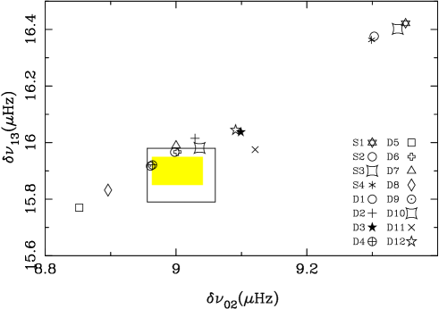
Figure 3: Comparison of observed and theoretical estimations of the two mean frequency differences $\delta\nu_{02}$ and $\delta\nu_{13}$.

In order to compare the seismic properties of the core of our models to those of the Sun, we have plotted on Fig. 3 the values of the two mean frequency differences $\delta\nu_{02}$ and $\delta\nu_{13}$. The mean observed values (see Table 1) and their corresponding errors are represented by the large box. The grey box corresponds to observations without IRIS values which have been obtained at larger solar activity. It is clear that for our solar models without microscopic diffusion these quantities are too large compared to the observed values while models with microscopic diffusion are in better agreement with the observations. However, the models D5 (with mild mass loss rate) and D8 (with a larger age) have a too small $\delta\nu_{02}$. This quantity is larger than the observed one for models D11 and D12 where opacity is computed with a heavy element abundance $Z_{k}$=$\cal Z$. Both penetrative convection and overshooting of the core in the early stage of solar evolution do not modify these parameters. Comparing the positions of models S2, D2 and D1 respectively to those of models S3, D3, D10, we note that the use of OPAL equation of state instead of CEFF equation of state slightly increases the values of both $\delta\nu_{02}$ and $\delta\nu_{13}$. On the other hand, these latter models which have the best physics are in a better agreement with the seismic sound speed as will be seen later on. A larger age or a smaller value of $Z/X$ could bring them in the observation box.

Globally the characteristic period $P_{0}$ for g modes are lower by about 1 minute for the solar models with microscopic diffusion compared to solar models without microscopic diffusion.

As exhibited in Fig. 2 and in Fig. 4 to 6, the microscopic diffusion increases the agreement between solar models and the seismic reference model. The dependence of the normalized frequency differences between the GONG frequencies and the theoretical frequencies on the degree $\ell$ is very weak, leading to a small dispersion of the curves in Fig. 2 (right). Globally the models D are close to the seismic reference model within $\pm 0.2\%$ for the sound speed and within $\pm 1\%$ for the density. In agreement with previous works (Gough et al. [1996], Christensen-Dalsgaard [1997]) the sound speed is lower than in seismic reference model below the convection zone. On the contrary, all our solar models with microscopic diffusion, but D3 and D12, present a systematic minimum on sound speed differences around the radius $R\sim 0.5R_{\odot}$. Moreover, below $R\sim 0.4R_{\odot}$ all our models except models D11, D12 have a sound velocity smaller than the seismic reference model. The negative minimum around $R\sim 0.2R_{\odot}$ which is present in most comparisons with inverse sound speeds, only appears as a small depression in our model D12 computed with OPAL equation of state and diffusion of Z with $Z_{k}={\cal Z}$.

Another consequence of the microscopic diffusion, as shown in Fig. 7, is that the evolutionary paths in the HR diagram of solar models with microscopic diffusion are shifted towards higher effective temperatures compared to the paths of solar models without microscopic diffusion.

Figure 4: Same as Fig. 1 for the solar models with microscopic diffusion D1 {CEFF, $Z_{\rm p}$} (thin full), D2 {CEFF, ${\cal X}_{\rm Z}$} (thick full), D3 {OPAL, ${\cal X}_{\rm Z}$} (thin dashed), D4 {CEFF, sMLR, $Z_{\rm p}$} (thick dashed), D5 {CEFF, mMLR, $Z_{\rm p}$} (thin dash-dot-dash).

Figure 5: Same as Fig. 1 for the solar models with microscopic diffusion D1 {CEFF, $Z_{\rm p}$} (thin full), D6 {CEFF, Un-shoot, $Z_{\rm p}$} (thick full), D7 {CEFF, Ov-shoot, $Z_{\rm p}$} (thin dashed), D8 {4.65 Gy, CEFF, $Z_{\rm p}$} (thick dashed), D9 {4.65 Gy, CEFF, $Z_{\rm p}$, 0.026} (thin dash-dot-dash).

Figure 6: Same as Fig. 1 for D3 {OPAL, ${\cal X}_{\rm Z}$} (thin full), D12 {OPAL, ${\cal Z}$} (thick full), D10 {OPAL, $Z_{\rm p}$} (thin dashed), D11 {OPAL, sMLR, ${\cal Z}$} (thick dashed) and D1 {CEFF, $Z_{\rm p}$} (thin dash-dot-dash); considering all constraints, D11 is our preferred model, but D12 without the lithium depletion constraint.

Figure 7: HR diagram for models D11 {OPAL, sMLR, ${\cal Z}$} (thin full), D12 {OPAL, ${\cal Z}$} (thick full), D1 {CEFF, $Z_{\rm p}$} (thin dashed), D10 {OPAL, $Z_{\rm p}$} (thick dashed), S2 {CEFF, OPAL95, PMS} (thin dash-dot-dash), S3 {OPAL, OPAL95, PMS} (thick dash-dot-dash) and S4 {OPAL, OPAL95, ZAMS} (thin dotted); an enlargement of the main sequence is plotted in the panel. At zero-age main sequence the models have about the same luminosities, the effective temperatures for solar models with microscopic diffusion exceed by $\sim 2\%$ those of solar models without microscopic diffusion. On the main sequence the evolutionary paths of S3 and S4 are superimposed.

5.2.1 Sensitivity to equation of state  and $Z_{\kappa}$

By inspection of Figs 4, 5, 6, it is seen that the relative sound speed differences with seismic reference model, have large variations of amplitude for models with CEFF equation of state with a pronounced minimum around $r=0.5R_{\odot}$. The behavior is much smoother for models with OPAL equation of state with a smaller minimum around $r=0.6R_{\odot}$. This could be partly due to the way partial recombination in the solar radiative interior is avoided in CEFF equation of state.

The model D10 (see Fig. 6) obtained with the equation of state OPAL, is located closer to the seismic reference model than the model D1 obtained with the equation of state CEFF, but for the density profiles, D1 is significantly closer than D10 to the seismic reference model. The differences in normalized frequencies are $\sim 1\mu$Hz between the two models. For the models D2 and D3 , the amount of heavy element $Z_{\kappa}$ used for the computation of opacities in models is taken as the abundance of the mean fictitious chemical ${\cal X}_{\rm Z}$. D2 is computed with the equation of state CEFF and D3 with OPAL. As seen Fig. 4, for the sound speed D3 is closer than D2 of the seismic reference model, and also for density except for $R\la 0.1R_{\odot}$. In agreement with Basu et al. ([1996]), however we find that the closest models to the seismic reference model are obtained with the opacities and equation of state OPAL.

Comparisons of models D3 ($Z_{\kappa}={\cal X}_{\rm Z}$), D10 ($Z_{\kappa}=Z_{\rm p}=Cte$) and D12 ($Z_{\kappa}=$ $\cal Z$) allow a comparison between the three approximations used for $Z_{\kappa}$. As far as the sound speed is concerned, the models computed with an opacity value taking into account of the diffusion of heavy element are closer to the seismic reference model than models with $Z_{\kappa}=Cte$; the models D3 and D12 are very similar, but for $R\la 0.2R_{\odot}$, D12 is closer to the seismic reference model. For the density, and $R\ga 0.1R_{\odot}$ the model D3 is closer to the seismic reference model than D10 and D12. Beneath the convection zone the sound velocity in model D12 is smaller than in D10 with a difference of the same amount, but of opposite sign, of those exhibited on Fig. 2(a) in Proffitt ([1994]), however, the physical inputs of that work differ from ours.

As a matter of conclusion, with the physical data used here, our study shows that the model computed with $Z_{\kappa}=$ $\cal Z$ has a sound speed profile closer to the seismic reference model than the model computed with $Z_{\kappa}={\cal X}_{\rm Z}$, and that is reversed for the density profile. The model D10 computed with $Z_{\kappa}=Cte$, though farther from the seismic reference model than D3 and D12, remains within $\pm 0.2\%$ for the sound speed and $\pm 1\%$ for the density. Therefore, using the seismic reference model, we are not able us to make a real discrimination between the three approaches employed to compute $Z_{\kappa}$, nevertheless our ”preferred” choice is $Z_{\kappa}=\$$\cal Z$.

5.2.2 Sensitivity to age and $(Z/X)_{\odot}$

According to Table 1 the present day solar age is known within 0.4 Gyr, the model D8 has been evolved 0.1 Gyr more than the model D1 using the same physics; in the same way, model D9 has been calibrated for a larger value of $(Z/X)_{\odot}=0.0260$ instead of $(Z/X)_{\odot}=0.0245$ for model D1. Figure 5 shows that the sound speed in D9 is systematically smaller than in D8 by $\sim 0.05\%$ i.e., about our limit of accuracy, except around the center, while the density in D9 is greater in the convection zone and in the core. The spread in normalized frequencies is $\sim 0.4\mu$Hz between the two models.

5.2.3 ${}^{7}{\rm Li}$ depletion due to undershoot and mass loss

All solar models with microscopic diffusion, except D4 and D5, reveal that the observed ⁷Li depletion does not only result from microscopic diffusion, even if, as for model D6, an undershooting factor equal to the upper limit of Basu & Antia ([1994]), namely $\zeta_{\rm un}=0.1H_{\rm p}$, is allowed for. The discontinuity of the temperature gradient due to undershooting is at the origin of spurious bumps, though within the global accuracy, namely $\pm 0.2\%$ for the sound speed and $\pm 0.5\%$ for density, as exhibited in Fig. 5. But Ahrens et al. ([1992]) have shown from models without microscopic diffusion that an undershooting factor $\zeta_{\rm un}\gse 0.3$ is needed to fit the present day observed lithium depletion; such a large amount is in conflict with the upper limit for $\zeta_{\rm un}$ derived from helioseismic observations (Basu & Antia [1994]; Monteiro et al. [1994]; Provost et al. [1996]). Our results for D6 (Table 4) also show that the most important amount of lithium depletion occurs during the pre-main sequence. This is in conflict with the observations of lithium in Pleiades and Hyades (see Sect. 3.5). The lithium being mostly destroyed in the hot core at the end of the pre-main sequence (Morel et al. [1996]) when the young Sun is still fully convective, a larger amount of undershooting will enhance the duration of this fully mixed stage and increase the pre-main sequence depletion. Therefore from the properties of our models it results that the ⁷Li depletion observed at present day in the solar photosphere does not only result from overshooting and microscopic diffusion.

In contrast in the models where the mass loss is included (models D4 and D5 of Table 4), the lithium depletion occurs mainly during the main sequence. The comparisons of theoretical sound speed and the density profiles with the seismic reference model (Fig. 5) show that the model D4 calculated with strong mass loss rate of Eq. (3), is closer to the seismic reference model than the model D5 computed with mild mass loss rate of Eq. (2). Indeed, stronger mass loss affects the structure of the present day model less because the mass loss phase is over faster. A model with strong mass loss rate becomes sensitive to the mass loss at the end of the pre-main sequence. Therefore, the evolutionary path in the HR diagram (Fig. 7) of the model D4 reaches the zero-age main sequence with decreasing effective temperature and luminosity. Indeed both the strong and the mild mass loss rates look as rather ad-hoc assumptions so we have not attempted to adjust the free parameters of these laws in order to fit accurately the present day observed lithium depletion. Nevertheless it appears that a strong mass loss rate is a promising process to explain the observed lithium depletion in the Sun as already claimed by Guzik & Cox ([1995]) despite the large expected neutrino capture rates and the marginal agreement with the observed frequency difference $\delta\nu_{02}$.

5.2.4 Overshoot of the convective core of the young Sun

The model D7 is computed with the physics of model D1 but with an overshooting of the convective core which appears during the early stage of solar evolution by a factor $\zeta_{\rm ov}=0.2$. The global properties of these models (Table 4) and the comparisons with the seismic reference model reveal only slight insignificant differences at center between D7 and D1 (Fig. 4 and Fig. 5) except a significant increase of the characteristic period $P_{0}$ of the gravity modes.

Table 4: Global characteristics of solar models with microscopic diffusion. $M_{\rm p}$ is the protosolar mass, $\zeta_{\rm ov}$ and $\zeta_{\rm un}$ respectively are the overshooting and undershooting factors; the other captions are given Table 3.

	D1	D2	D3	D4	D5	D6	D7	D8	D9	D10	D11	D12
$M_{\rm p}$	1.	1.	1.	1.1	1.095	1.	1.	1.	1.	1.	1.11	1.
$l/H_{\rm p}$	2.00	1.95	1.97	2.00	2.01	2.00	2.00	2.02	2.02	1.97	1.93	1.92
$\zeta_{\rm ov}$							0.2
$\zeta_{\rm un}$						0.1
$Y_{\rm p}$	0.276	0.276	0.276	0.275	0.273	0.275	0.276	0.275	0.279	0.273	0.273	0.274
$Z_{\rm p}$	0.0191	0.0191	0.0191	0.0191	0.0189	0.0190	0.0191	0.0191	0.0201	0.0191	0.0194	0.0196
$(Z/X)_{\rm p}$	0.0271	0.0271	0.0271	0.0270	0.0267	0.0269	0.0271	0.0271	0.0286	0.0270	0.0276	0.0277
$X_{\rm nCNO}$	0.0053	0.0053	0.0052	0.0052	0.0050	0.0051	0.0052	0.0053	0.0063	0.0052	0.0056	0.0058
LiZAMS	3.00	3.01	2.95	3.13	3.13	2.74	3.00	2.99	2.99	2.88	3.13	2.95
$Y_{\odot}$	0.247	0.246	0.244	0.247	0.247	0.248	0.247	0.246	0.250	0.244	0.245	0.245
$Z_{\odot}$	0.0179	0.0179	0.0180	0.0179	0.0179	0.0179	0.0179	0.0180	0.0189	0.0180	0.0180	0.0180
Li⊙	2.92	2.94	2.88	2.17	1.96	2.66	2.92	2.92	2.92	2.81	1.92	2.88
$R_{\rm ZC}$	0.710	0.713	0.711	0.713	0.709	0.702	0.710	0.708	0.709	0.707	0.710	0.711
$T_{\rm c}$	1.557	1.559	1.557	1.558	1.560	1.556	1.557	1.560	1.563	1.556	1.562	1.565
$\rho_{\rm c}$	151.5	150.8	150.2	152.0	153.9	151.5	150.8	153.1	156.3	150.9	150.6	151.2
$Y_{\rm c}$	0.637	0.637	0.635	0.639	0.644	0.637	0.634	0.642	0.641	0.635	0.639	0.638
$Z_{\rm c}$	0.0200	0.0201	0.0202	0.0200	0.0199	0.0199	0.0201	0.0201	0.0210	0.0201	0.0207	0.0208
$\Phi_{\rm Ga}$	128	128	128	136	140	128	128	129	130	127	144	130
$\Phi_{\rm Cl}$	7.72	7.81	7.68	8.25	8.69	7.68	7.74	7.93	8.20	7.58	8.93	8.27
$\Phi_{\rm Ka}$	0.61	0.62	0.61	0.66	0.69	0.61	0.61	0.63	0.66	0.60	0.72	0.66
$\delta\nu_{02}$	9.00	9.03	9.10	8.96	8.85	9.00	9.00	8.90	8.96	9.04	9.13	9.09
$\delta\nu_{13}$	15.96	16.01	16.04	15.92	15.77	15.97	15.99	15.83	15.92	15.98	15.98	16.04
$P_{0}$	35.73	35.82	35.87	35.63	35.27	35.76	35.97	35.43	35.65	35.78	35.76	35.75

6 Conclusions

We have computed solar models with our stellar evolution code CESAM and using updated physics. Our models are attempts to extend the study of the sensitivity of solar models with microscopic diffusion to pre-main sequence, lithium depletion, mass loss, microscopic diffusion of heavy species, overshooting and undershooting. Effects of rotation and of turbulent diffusion are ignored here. We have compared the sound speed and the density profiles of the seismic reference model of Basu et al. ([1996]) to calibrated solar model computed with various opacity data, equation of state, microscopic diffusion, mass loss rate, undershooting and overshooting amounts. The solar models with microscopic diffusion agree with the seismic model within $\pm 0.2\%$ for the sound speed and $\pm 1\%$ for density, while for the solar models without microscopic diffusion the agreement is hardly better than $\pm 1\%$ and $\pm 10\%$ respectively for the sound speed and density. For the solar models with microscopic diffusion the depth of the convection zone and the amount of helium at surface agree fairly well with their values inferred by helioseismology. A significant increase of the quality of solar models results from the recent improvements of opacities and equation of state, any amelioration of solar models will necessitate to take fully into account the changes of chemicals in opacities and equation of state.

Our models reveal that the lithium depletion observed at solar surface is certainly not due to undershooting at the bottom of the convection zone and can be explained by a strong mass loss occurring during the first 200 Myr; however, in the solar models described in this paper the turbulent diffusion induced either by the rotation or by the internal waves has not been taken into account.

Considering all the observational and helioseismologic constraints our preferred model is D11 computed with strong mass loss rate, OPAL opacities and equation of state, microscopic diffusion of hydrogen, helium and, as trace elements, all the CNO species plus a fictitious mean no-CNO chemical which models the microscopic diffusion of the heaviest elements of the mixture; but if one excludes the constraint on the lithium depletion, our preferred model is D12 computed with the same physics but without mass loss. However, in the present state of art, the precision of solar models needs to be still improved by one magnitude in order to reach the accuracy of the solar data inferred by helioseismology.

Appendix A Calculation of abundances

The opacities and equation of state are tabulated for mixtures with various amounts of hydrogen $X_{\rm H}$, and heavy element content $Z$; the ratios between the species of which $Z$ is made of are fixed; along the solar evolution these ratios are modified by thermonuclear reactions and microscopic diffusion. Therefore, using the available data for opacities and equation of state, a difficulty is the estimate of $Z$ as consistently as possible. At time $t$, $X_{i}$, the amount per unit of mass of the species labelled with $i=1,\ldots,N_{c}$ ($N_{c}$ is the total number of chemicals) is written:

$$X_{i}=\frac{n_{i}M_{i}m_{u}}{\sum_{j=1}^{N_{c}}n_{j}M_{j}m_{u}}=\frac{n_{i}M_{i}m_{u}}{\rho}$$

and

$$1\equiv\sum_{j=1}^{N_{c}}X_{i}=X_{\rm nCNO}+\sum_{j=1}^{N}X_{i}$$ (4)

here, $n_{i}$ is the number density, $M_{i}$ is the atomic mass of $X_{i}$, $M_{i}\in\bbbr$ differs from the integer atomic number $A_{i}$, (Clayton [1968]), $m_{u}$ is the atomic mass unit, $N\leq N_{c}$ is the number of species entering into the nuclear network, $X_{\rm nCNO}$ is the amount, per mass unit, of a fictitious mean heavy element of mean atomic mass $M_{\rm nCNO}$ which does not belong to the nuclear network and $\rho$ is the density. Therefore $Z$ is writen:

$$Z\equiv 1-X_{\rm H}-X_{\rm He}=X_{\rm nCNO}+\sum_{j\not={\rm H,He}}X_{j};$$

for sake of clarity the labels ”H” and ”He” are used in place of integer indexes; $X_{\rm H}$ and $X_{\rm He}$ also include, respectively, the isotopes of hydrogen and helium, (see Appendix B). Following Fowler et al. ([1975]), we use the number of mole g^-1, $Y_{i}\equiv X_{i}/M_{i}$; then the amount, per unit of mass, of the species indexed with $i$ is written:

$$X_{i}=\frac{Y_{i}M_{i}}{Y_{\rm nCNO}M_{\rm nCNO}+\sum_{j=1}^{N}Y_{j}M_{j}},$$

namely the abundances of hydrogen, and heavy element which are entries of opacities or equation of state, are respectively written:

$$X_{\rm H} = \frac{Y_{\rm H}M_{\rm H}}{Y_{\rm nCNO}M_{\rm nCNO}+\sum_{j=1}^{N}Y_{j}M_{j}},$$

$$Z = \frac{Y_{\rm nCNO}M_{\rm nCNO}+\sum_{j\not={\rm H,He}}Y_{j}M_{j}}{Y_{\rm nCNO}M_{\rm nCNO}+\sum_{j=1}^{N}Y_{j}M_{j}}$$ (5)

therefore Eq. (4) is fullfilled, despite the fact that the quantity which is conserved is the nucleon number expressed as:

$$0\equiv\sum_{i=1}^{N}A_{i}{dX_{i}\over dt}=\sum_{i=1}^{N}A_{i}M_{i}{dY_{i}\over dt},$$

The similar approach of Richard et al. ([1996]) uses the normalization equation:

$$1\equiv X_{\rm H}+\sum_{i\not={\rm H}}X_{i}+Z.$$

Figure 8: Relative differences for heavy element contents $Z$ (top), $\kappa$ opacities (middle) and $C$ sound velocities (bottom) along the normalized radius, between the model S1 and solar models without microscopic diffusion in which ³He either, is, Sy (full) or, is not, Sz (dash-dot-dash), included into the helium content for opacities calculations.

Appendix B ³He abundance, equation of state and opacities

In main sequence solar models, a local maximum of ³He, occurs around $R\sim 0.3R_{\odot}$, it amounts to 10% of the local helium content, there $X_{{}^{3}{\rm He}}\sim Z$; this effect needs to be taken into account in the calculation of $Z_{\kappa}$; Fig. 8 exhibits the fractional differences on $Z_{\kappa}$, opacity and sound velocity between the model S1 used as a reference – for S1, $Z_{\kappa}\equiv Cte$ (see Table 2) – and solar models without microscopic diffusion (not detailed here for sake of briefness) calculated with and without ³He included into the helium content i.e., $Z_{\kappa}\equiv 1-^{1}$H$-^{3}$He$-^{4}$He and $Z_{\kappa}\equiv 1-^{1}$H$-^{4}$He. From Fig. 8 the fractional differences on sound speeds are of the order of $\pm 3\times 10^{-3}$ i.e., of the order of accuracy achieved with solar models with microscopic diffusion. Likewise Fig. 9 shows that the spread of O-C frequencies between sets of modes of constant $\ell$ computed between GONG observations decreases by taking (left) $Z\equiv 1-^{1}$H$-^{3}$He$-^{4}$He instead of (right) $Z\equiv 1-^{1}$H$-^{4}$He. The difference of the sound speed below the convection zone and around $R\sim 0.3R_{\odot}$ seen in Fig. 8 induces scaled frequency difference between the two models of the order of $1\,\mu$Hz, as seen in Fig. 10.

Figure 9: O-C frequencies between sets of modes of constant $\ell$ computed between GONG observations and solar models without microscopic diffusion computed respectively with, $Z=1-^{1}$H$-^{4}$He (Sz) and $Z\equiv 1-^{1}$H$-^{3}$He$-^{4}$He (Sy).

Figure 10: Scaled frequencies differences between the models Sy and Sz of Fig. 9 for modes of low degree ($\ell$= 0, 1, 2, 3, 4, 5, 10; dotted), intermediate degree ($\ell$= 20, 30, 40, 50; full) and high degree ($\ell$= 70 100 120 140; dashed).

Everywhere, but around $\simeq 0.3R_{\odot}$, the small abundance of ³He has no effect on opacities and equation of state; around $R\simeq 0.3R_{\odot}$ opacities and equation of state are mainly sensitive to free-free transitions, there ³He and ⁴He are equivalent providers of electrons; therefore it is relevant to include ³He in the helium content for the calculation of opacities. Similar phenomenon prevails for all components of $Z$ which present noticeable changes of abundances due to nuclear reactions and diffusion e.g., for ¹²C and ¹⁴N if $R\lse 0.2R_{\odot}$. The sensitivity of the sound velocity to such effect being of same order of the accuracy reached by solar models with microscopic diffusion, we emphasize that any improvement of that accuracy will necessitate opacities – even equation of state – taking into account the changes of mixture.