Spatial distribution of the accretion luminosity of isolated neutron stars and black holes in the Galaxy

Abstract

We present here a computer model of the distribution of the luminosity, produced by old isolated neutron stars and black holes accreting from the interstellar medium in the Galaxy in $R$–$Z$ plane. We show that the luminosity distributions have a toroidal structure, with the maximum at $\approx 5-6kpc$.

1 Introduction

Old isolated neutron stars (NS) and black holes (BH) form a big populations of the galactic sources (about $10^{8}$–$10^{9}$ objects in the Galaxy), but most of them are unobserved today. Less than $10^{3}$ of young NS appear as radiopulsars, and no isolated BH are observed at the present moment (probably, some of them were detected, for example, in the $ROSAT$ survey, but no one is identified). As in this article we will speak only about isolated compact objects, we will not use that adjective: “isolated” for NS and BH.

During the last several years, the spatial distribution and other properties of NS became of great interest, because as it has been proposed, NS can be observed by the ROSAT sattelite in soft X-rays due to accretion from the interstellar medium (ISM) (see, for example, Treves & Colpi 1991), and several sources of this type have been observed (Walter et al. 1996). BH also can appear as such X-ray sources (Heckler & Kolb 1996) with some differences in spectrum and temporal behaivour (absence of pulsations, for example). That’s why here we try to obtain a picture of the distribution of the accretion luminosity of these sources.

Fast rotation and/or strong magnetic field can prevent accretion onto the surface of the NS. In this case the X-ray luminosity will be very low (except the case of the transient source formation due to the envelope around the NS) (see Popov 1994 and Lipunov & Popov 1995). Here we consider only accreting NS. Most of NS are on the stage of accretion, because their magneto-rotational evolution usually finishes at this stage approximately $10^{8}$ years after their birth. The NS properties (periods etc) on the stage of accretion depend upon the magnetic field decay (see Konenkov & Popov 1997). BH, of course, can appear only as Accretors.

In the articles of Gurevich et al. (1993), Postnov & Prokhorov (1993, 1994) it was shown that NS in the Galaxy form a toroidal structure. The distribution of the ISM (see, for example, Bochkarev 1993) also has the toroidal structure. The maxima of both distributions roughly coincide.

Therefore, most part of NS (and, as one can say, BH) is located in the dence regions of the ISM. Thus the accretion luminosity in these regions should be higher. The results of computer simulations of this situation are presented in this paper.

The trajectories of NS and BH were computed directly for specified initial velocity distribution, the Galaxy gravitational potential and the distribution of the ISM density. Preliminary results of such computations for NS for $\delta$–function and maxwellian velocity distributions were presented in Popov & Prokhorov (1996, paper I).

In the section 2 we briefly describe our model. In the third section the results and a short discussion are presented. And finaly we conclued our results in the last section.

2 The Model

We solved numerically the system of differential equations of motions in the given potential.

We used the Galactic potential, taken in the form (Paczynski 1990):

$$\Phi_{i}(R,Z)=GM_{i}/\left(R^{2}+[a_{i}+(Z^{2}+b_{i}^{2})^{1/2}]^{2}\right)^{1/2}$$

with a quasi-spherical halo with the density distribution in the form:

$$\rho=\frac{\rho_{0}}{1+(d/d_{0})},\,\,\,d^{2}=R^{2}+Z^{2}.$$

Here $R$ and $Z$ are cylindrical coordinates, $d$– radial distance in the quasi-spherical halo. The parameters of the potential are given in the table, $\rho_{0}$ is determined through the halo mass, $M_{0}$.

Disk	$a_{D}$=0	$b_{D}$=277 pc	$M_{D}=1.12\cdot 10^{10}M_{\odot}$
Bulge	$a_{B}$=3.7 kpc	$b_{B}$=200 pc	$M_{B}=8.07\cdot 10^{10}M_{\odot}$
Halo		$d_{0}$=277 pc	$M_{0}=5.0\cdot 10^{10}M_{\odot}$

The density in our model was constant in time. Local density was calculated using data and formulae from Bochkarev (1993) and Zane et al. (1995). Here $R$ and $Z$ are cylindrical coordinates (it is assumed, that the Galaxy has cylindrical symmetry), $n$ – total concentration, $n_{HI}$ and $n_{H_{2}}$ are concentrations of the neutral and molecular hydrogene, $n_{0}(R)$, $n_{2}(R)$ and $n_{3}(R)$ are the values of concentrations for $Z=0$.

$$n(R,Z)=n_{HI}+2\cdot n_{H_{2}}$$

$$n_{H_{2}}=n_{2}(R)\cdot exp\left[\frac{-Z^{2}}{2\cdot(70pc)^{2}}\right]$$

If $0kpc\leq R\leq 3.4kpc$, then

$$n_{HI}=n_{0}(R)\cdot exp\left[\frac{-Z^{2}}{2\cdot(140pc\cdot R/2kpc)^{2}}\right],$$

For $0kpc\leq R\leq 2kpc\,\,n_{0}(R)$ was assumed to be constant for all $R$:

$$n_{0}(R<2kpc)=n(R=2kpc)$$

Of course, it is not accurate for small R, so for the very central part of the Galaxy our results are only a rough estimation (see Zane et al. (1996) for detailed calculation of NS emiision from the Galactic center region). If $3.4kpc\leq R\leq 8.5kpc$, then

$$n_{HI}=0.345\cdot exp\left[\frac{-Z^{2}}{2\cdot(212pc)^{2}}\right]+$$

$$0.107\cdot exp\left[\frac{-Z^{2}}{2\cdot(530pc)^{2}}\right]+$$

$$0.064\cdot exp\left[\frac{-Z}{403pc}\right]$$

If $8.5\leq R\leq 16kpc$, then

$$n_{HI}=n_{3}(R)\cdot exp\left[\frac{-Z^{2}}{2\cdot(530pc\cdot R/8.5kpc)^{2}}\right]$$

$n_{0}(R)$, $n_{2}$ and $n_{3}(R)$ were taken from Bochkarev (1993).

The density distribution in the $R$-$Z$ plane used in our computations is shown in the figure 1.

Figure 1: The density distribution in units particle per cubic centimeter in the $R$–$Z$ plane.

In our model we assumed, that the birthrate of NS and BH is proportional to the square of the local density. Stars were born in the Galactic plane (Z=0) with circular velocities plus additional isotropic kick velocities.

For the kick velocity we used the formula from Lipunov et al. (1996). It was constructed as an analitical approximation of the three-dimensial velocity distribution of radiopulsars from Lyne & Lorimer (1994).

$$f_{LL}(V)\propto\frac{x^{0.19}}{(1+x^{6.72})^{1/2}},$$

here $V$– spatial velocity of the compact object, $V_{char}$ – characteristic velocity, $x=V/V_{char}$, $f_{LL}$– the probability (see the detail describtion of the analitical approximation in Lipunov et al. (1996)). This formula reproduces the observed distribution with the mean velocity 350 km/s for $V_{char}$=400 km/s. This velocity distribution seems more luckely, than the $\delta$–function and Maxwellian distributions, which we used in Paper I. Kick velocities were taken equal for NS and BH (this is a “zero-hypothesis”, as we don’t have any exact information on this matter). But it is possible, that BH have lower kick velocities because of their high masses. One of the reasons to make computations for $V_{char}$=200 km/s was to explore this situation.

For each star we computeded the exact trajectory and the accretion luminosity. The accretion luminosity was calculated using Bondi formula:

$$L=\left(\frac{GM\dot{M}}{R_{lib}}\right)$$

$$\dot{M}=2\pi\left(\frac{(GM)^{2}\rho(R,Z)}{(V_{s}^{2}+V^{2})^{3/2}}\right)$$

.

Sound velocity,$V_{s}$, was taken to be 10 km/s everywhere. We used equal masses $M_{NS}=1.4M_{\odot}$ for NS and $M_{BH}=10M_{\odot}$ for BH. Density is determined as: $\rho=n\cdot m_{H}$, where $m_{H}$– the mass of the hydrogen atom. Radii, $R_{lib}$, where the energy is libirated, were assumed to be equal to 10 km for NS and 90 km (i.e. $3\cdot R_{g}$, $R_{g}=2GM/c^{2}$) for BH. Statistics was collected on the grid with the cell size 100 pc in R-direction and 10 pc in Z-direction (centered at R=50 pc, Z=5 pc and so on). The luminosity is shown on the graphs in ergs per second per cubic parsec.

For the normalization of our results we used an assumption, that there are $N_{NS}=10^{9}$ NS and $N_{BH}=10^{8}$ BH in the calculated volume of the Galaxy. For Salpeter mass function with $\alpha$=2.35 the ratio of NS to BH is about 10 if NS are formed from the stars with masses between $10M_{\odot}$ and $\approx 45-50M_{\odot}$, and BH from the stars with masses higher than $\approx 45-50M_{\odot}$. Motch et al. (1997) argued, that $N_{ns}=10^{9}$ can be ruled out, and $N_{NS}=10^{8}$ is a more probable value, but for the caclculations of the distribution the total number is not so improtant, and for other numbers of compact objects the results (i.e. the value of the luminosity) can be easily scaled.

3 Results and discussion

On the figures 2–5 we represent the results for two characteristic values of the velocity distribution for NS and BH. On the graphs 2–5 the region $16000\,pc\,\times\,800\,pc$ for averaged accretion luminosity for the azimutale angle 0–180 degrees is shown. We show only this region, because we are mainly interested in the part, where the maximum is situated, but while the computations NS and BH could move inside infinite region. The scale for $R$ and $Z$ axes are different in order to show clearly the structure in $Z$ direction. Differences between the luminosity distribution for $Z>0$ and $Z<0$ demonstrate accuracy of the computations (curves were not smoothed).

Figure 2: The accretion luminosity distribution in $R$–$Z$ plane for neutron stars for characteristic kick velocity 200 km/s. The luminosity is shown in ergs per second per cubic parsec. $N_{NS}=10^{9}$

Figure 3: The accretion luminosity distribution in the $R$–$Z$ plane for neutron stars for characteristic kick velocity 400 km/s. The luminosity is shown in ergs per second per cubic parsec. $N_{NS}=10^{9}$

Figure 4: The accretion luminosity distribution in the $R$–$Z$ plane for black holes for characteristic kick velocity 200 km/s. The luminosity is shown in ergs per second per cubic parsec. $N_{BH}=10^{8}$

Figure 5: The accretion luminosity distribution in the $R$–$Z$ plane for black holes for characteristic kick velocity 400 km/s. The luminosity is shown in ergs per second per cubic parsec. $N_{BH}=10^{8}$

On the figure 6 the slice at Z=+5 pc (the first grid cells in the positive Z-direction) for the characteristic kick velocity $V_{char}$= 200 km/s is shown: luminosity vs. radius. The figure is not symmetric. The right part corresponds to the azimutale angles 0–180 degrees, the left - 180–360 degrees. Differences between the left and the right parts of the curve demonstrate how precise our method is.

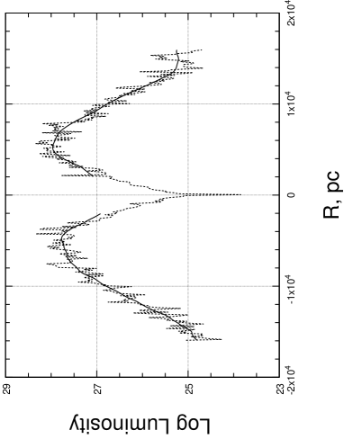
Figure 6: Slice at Z=+5 pc for NS for the characteristic kick velocity 200 km/s. $N_{NS}=10^{9}$. The accretion luminosity is shown in ergs per second per cubic parsec. With the solid line we show the smoothed curve.

4 Concluding remarks

As it is clearly seen from the figures, the distribution of the accretion luminosity in R-Z plane forms a toroidal structure with the maximum at approximatelly 5 kpc.

As expected, for BH we have relatively higher luminosity, than for NS, as BH have greater masses. But if the total number of BH is significantly lower than the number of NS, their contribution to the luminosity can be less than the contribution of NS. The total accretion lumiunosity of the Galaxy for $N_{NS}=10^{9}$ and $N_{BH}=10^{8}$ is about $10^{39}-10^{40}$erg/s. For the characteristic velocity 200 km/s for NS the maximum of the distribution is situated approximately at 5.0 kpc and for BH at 4.8 kpc. For NS with the characteristic velocity 400 km/s maximum is situated at 5.4 kpc, and for BH at 5.0 kpc. This result is also expected because of the same reason (higher masses of the BH with the same value of kick velocity).

The toroidal structure of the luminosity distribution of NS and BH is an interesting and important feature of the Galactic potential. As one can suppose, for low characteristic kick velocities and for BH we obtained higher luminosity.

As me made very general assumptions, we argue, that such a distribution is not unique only for our Galaxy, and all spiral galaxies can have such a distribution of the accretion luminosity, associated with accreting NS and BH.

- [1] Bochkarev, N.G. , 1992 ”Basics of the ISM physics”, Moscow, Moscow State Univ. Press
- [2] Gurevich, A. V., Beskin, V. S., Zybin, K. P., & Ptitsyn, M. O., 1993, ZhETF, 103, 1873
- [3] Heckler, A.F. & Kolb, E.W., 1996, ApJ 472, L85
- [4] Konenkov D.Yu., & Popov, S.B., 1997, PAZh, 23 (in press)
- [5] Lipunov, V.M. & Popov, S.B., 1995, AZh, 71, 711
- [6] Lipunov, V.M., Postnov,K.A. & Prokhorov, M.E., 1996, A&A, 310, 489
- [7] Lyne, A.G. & Lorimer, D.R., 1994, Nat 369, 127
- [8] Motch C., Guillout P., Haberl F., Pakull M., Pietsch W. & Reinsch K., 1997, A & A, 318, 111
- [9] Paczynski, B., 1990, ApJ 348, 485
- [10] Popov, S.B., 1994, Astron. Circ., N1556, 1
- [11] Popov, S.B. & Prokhorov, M.E., 1996, astro-ph/9609126, (A & A Trans. in press ) (paper I)
- [12] Prokhorov, M.E. & Postnov, K.A., 1994, A & A, 286, 437
- [13] Prokhorov, M.E. & Postnov, K.A., 1993, A & A Trans., 4, 81
- [14] Treves, A. & Colpi, M., 1991, A & A, 241, 107
- [15] Walter, F.M., Wolk, S.J., & Neuhauser, R., 1996, Nat , 379, 233
- [16] S. Zane, S., Turolla, R., Zampieri, L., Colpi, M., & Treves, A., 1995, ApJ, 451, 739
- [17] Zane, S., Turolla, R., & Treves, A., 1996, ApJ, 471, 248