Collimation of Highly Variable Magnetohydrodynamic Disturbances around a Rotating Black Hole

Abstract

We have studied non-stationary and non-axisymmetric perturbations of a magnetohydrodynamic accretion onto a rotating (Kerr) black hole. Assuming that the magnetic field dominates the plasma accretion, we find that the accretion suffers a large radial acceleration resulting from the Lorentz force, and becomes highly variable compared with the electromagnetic field there. In fact, we further find an interesting perturbed structure of the plasma velocity with a large peak in some narrow region located slightly inside of the fast-magnetosonic surface. This is due to the concentrated propagation of the fluid disturbances in the form of fast-magnetosonic waves along the separatrix surface. If the fast-magnetosonic speed is smaller in the polar regions than in the equatorial regions, the critical surface has a prolate shape for radial poloidal field lines. In this case, only the waves that propagate towards the equator can escape from the super-fast-magnetosonic region and collimate polewards as they propagate outwards in the sub-fast-magnetosonic regions. We further discuss the capabilities of such collimated waves in accelerating particles due to cyclotron resonance in an electron-positron plasma.

Hirotani Collimation of MHD Disturbances around Rotating Black Hole

1 Introduction

It is commonly accepted that extragalactic jets are intimately linked with accretion process onto supermassive black holes residing in the central regions of active galactic neuclei. These jets are initially relativistic, as indicated by superluminal proper motions of radio emitting knots (e.g., Wehrle et al. 1992) and by high-energy, rapidly variable $\gamma$-ray emissions (e.g., Montigny et al. 1995). Moreover, Hobble Space Telescope studies of the base of M87 jet reveal a rotating gas disk apparently lying normal to the jet direction (Ford et al. 1994; Harms et al. 1994). Despite intense study, the underlying formation mechanism is still uncertain. Nevertheless, hydrodynamic and magnetohydrodynamic processes associated with the accretion disk seem to be a promising candidate mechanism.

Possible flows of the energy conversion from the accretion to a small fraction of gas in jets have been suggested by Shakura and Sunyaev (1973) in the context of a thick supercritical accretion disk which exhibites inflow along the equator and outflow near to the poles. If the radiation-supported rotating gas adopts a hydrostatic toroidal configuration, then a pair of funnels are defined which could be responsible for the production of jets along the rotational axis (Lynden-Bell 1978). Blandford and Payne (1982) considered a magnetized disk and showed that a gas leaves the disk in a centrifugally driven wind provided that the magnetic field makes an angle of less than $60^{\circ}$ with the radius vector at the disk. Furthermore, the magnetohydrodynamic (MHD) disturbances produced at a galactic nucleus with a compact nuclear disk would be strongly collimated polewards resulting in jets, if the Alfvén velocity in the disk is much higher than its surroundings (Sofue 1980). Such a collimation would lead to an increase in the wave amplitude, resulting in shock waves which are conjectured to develop into a strongly compressed region of the magnetic field. In this region, high-energy particles are likely to be accelerated in the perpendicular direction to the equatorial nuclear disk.

The purpose here is to explore the issue whether MHD waves can convey some portions of accretion energy to the polar regions in the vicinity of a black hole. Causality requires that the MHD inflows should pass through the fast-magnetosonic point and become super-fast-magnetosonic at the horizon. The investigation of the so-called critical condition that the inflow should pass through this point smoothly offers, in fact, the key to an understanding of MHD interactions in a black hole magnetosphere.

The MHD interactions are expected to work most effectively in the magnetically dominated limit in which the rest-mass energy density of particles is negligible compared with the magnetic energy density. In this limit, the fast-magnetosonic point is located very close to the horizon (e.g., Phinney 1983); as a result, a general relativistic treatment is required. Analyzing the critical condition in a stationary and axisymmetric magnetically dominated black hole magnetosphere, Hirotani et al. (1992, hereafter Paper I) showed that roughly $10\%$ of the rest-mass energy and a significant fraction of the initial angular momentum are transported from the fluid to the magnetic field during the infall. Furthermore, if a small-amplitude perturbation is introduced into the magnetosphere, a lot of perturbation energy is deposited from the magnetic field to the fluid near to the fast-surface in the short-wavelength limit; accordingly, the plasma accretion becomes highly variable there ([Hirotani et al. 1993], hereafter Paper II). Subsequently, Hirotani and Tomimatsu (1994, Paper III) investigated the spatial structure of the disturbance in a Schwarzschild metric, assuming that the characteristic scale of the radial variations of perturbed quantities is comparable to that of unperturbed quantities instead of adopting the short-wavelength limit. They revealed that the magnetically dominated accretion becomes most variable at the fast-magnetosonic separatrix surface and that the large-amplitude fluid’s disturbance can escape into the sub-fast-magnetosonic regions by propagating meridionally almost along the separatrix. In this paper, we extend the analysis performed in Paper III to a Kerr metric, further examine the propagation of the escaped fast waves in the sub-fast regions, and discuss the possibilities of particle acceleration due to a collimation of such waves.

The outline of this paper is as follows. In §2, we formulate non-stationary non-axisymmetric perturbations of the MHD accretion and derive the wave equation describing the perturbation. Solving the wave equations, we show in §3 that the fluid becomes most variable slightly inside of the fast-surface, which is consistent with the results obtained in Paper II and III. We further demonstrate that the disturbances can escape into the sub-fast regions in the form of fast waves by propagating towards the equator provided that the fast-magnetosonic speed, $U_{\rm FM}$ is slower in the polar regions than in the equatorial regions. In §4, the escaped fast waves will be shown to collimate towards the rotational axis under such a distribution of $U_{\rm FM}$. We finally discuss the capabilities of such collimated waves in accelerating of particles due to nonlinear interactions between the waves and electron-positron plasmas in §5.

2 Magnetically Dominated Accretion

We will begin by considering basic equations describing a magnetosphere around a rotating black hole. Since the self-gravity of the electromagnetic field and plasma around a black hole is very weak, the background geometry of the magnetosphere is described by the Kerr metric,

$$ds^{2} = {\Delta-a^{2}\sin^{2}\theta\over\Sigma}dt^{2}+{4Mar\sin^{2}\theta\over\Sigma}dtd\phi$$ (1)

$$-{A\sin^{2}\theta\over\Sigma}d\phi^{2}-{\Sigma\over\Delta}dr^{2}-\Sigma d\theta^{2},$$

where $\Delta\equiv r^{2}-2Mr+a^{2}$, $\Sigma\equiv r^{2}+a^{2}\cos^{2}\theta$, $A\equiv(r^{2}+a^{2})^{2}-\Delta a^{2}\sin^{2}\theta$ and $a\equiv J/M$; $M$ is the mass of a hole. Throughout this paper we use geometrized units such that $c=G=1$.

Under ideal MHD conditions, since the electric field vanishes in the fluid rest frame, we have $F_{\mu\nu}U^{\mu}=0$, where $F_{\mu\nu}$ is the electromagnetic field tensor satisfying Maxwell equations, $F_{[\mu\nu,\rho]}=0$ and $U^{\mu}$ is the fluid four velocity. The motion of the fluid in the cold limit is governed by the following equations of motion:

$$T^{\mu\nu}{}_{;\nu} = \Biggl{[}\mu nU^{\mu}U^{\nu}+{1\over 4\pi}\bigl{(}F^{\mu\rho}F_{\rho}{}^{\nu}+{1\over 4}g^{\mu\nu}F_{\alpha\beta}F^{\alpha\beta}\bigr{)}\Biggr{]}_{;\nu}$$ (2)

$$= 0,$$

where the semicolon denotes a covariant derivative and $\mu$ the rest-mass of a particle. For electron-proton plasmas $\mu$ refers to a rest-mass of a proton, whereas for electron-positron plasmas $\mu$ refers to that of an electron (or a positron). The proper number density ($n$) obeys the continuity equation, $(nU^{\mu})_{;\mu}=0$. We adopt these basic equations for a description of stationary and axisymmetric black-hole magnetospheres in §2.1 and for an analysis of perturbed state in §2.2 and afterwards.

2.1 Unperturbed Magnetosphere

From an analysis of the stationary and axisymmetric ideal MHD equations, it is known that there exist four integration constants that are conserved along each flow line (e.g., [Bekenstein and Oron (1978)]; Camenzind 1986a,b). These conserved quantities are the angular velocity of a magnetic field line ($\Omega_{F}$), the particle flux per magnetic flux tube ($\eta$), the total energy ($E$) and the total angular momentum ($L$) per particle. They are defined as follows:

$$\Omega_{F}={F_{tr}\over F_{r\phi}}={F_{t\theta}\over F_{\theta\phi}},$$ (3)

$$\eta = -{\sqrt{-g}nU^{r}\over F_{\theta\phi}}=-{\sqrt{-g}nU^{\theta}\over F_{\phi r}}$$ (4)

$$= -{\sqrt{-g}n(U^{\phi}-\Omega_{F}U^{t})\over F_{r\theta}},$$

$$E\equiv\mu U_{t}-{\Omega_{F}\over 4\pi\eta}B_{\phi}$$ (5)

and

$$L=-\mu U_{\phi}-{1\over 4\pi\eta}B_{\phi},$$ (6)

where the toroidal magnetic field ($B_{\phi}$) is defined by

$$B_{\phi}=-{\rho_{\rm w}{}^{2}\over\sqrt{-g}}F_{r\theta};$$ (7)

$$\rho_{\rm w}{}^{2}\equiv\Delta\sin^{2}\theta,\qquad\sqrt{-g}\equiv\Sigma\sin\theta.$$ (8)

When $0<\Omega_{\rm F}<\Omega_{\rm H}$ holds, thereby hole’s rotational energy and angular momentum are extracted magnetohydrodynamically (Blandford and Znajek 1977; Phinney 1983), both $E$ and $L$ become negative. A poloidal flow line is identical with a poloidal magnetic field line, and is given by $\Psi(r,\theta)=$ constant, where $\Psi$ is the $\phi$-component of the unperturbed electromagnetic vector potential. The conserved quantities are functions of $\Psi$ alone.

We next describe a stationary plasma accretion in a black-hole magnetosphere. In a black-hole magnetosphere there are two light surfaces. One is called the outer light surface, which is formed by centrifugal force in the same manner as in pulsar models. The other is called the inner light surface, which is formed by the gravity of the hole. In a region between the horizon and the inner light surface, the plasma must stream inwards, while in a region beyond the outer light surface it must stream outwards. A plasma source in which both inflows and outflows start with a low poloidal velocity is located between these two light surfaces (Nitta et al. 1991); the injection region ($r={r}_{\rm I}$) of the accretion may be a pair-creation zone above the disk (Beskin et al. 1992; Hirotani and Okamoto 1997) or the disk surface whose inner edge corresponds to the innermost stable circular orbit in a Kerr geometry. Along the magnetic field lines the plasma inflows pass through the Alfvén point, the light surface, and the fast magnetosonic point ($r={r}_{\rm F}$), successively; they finally reach the event horizon ($r={r}_{\rm H}$). From now on we use the subscripts I, F and H to indicate that the quantities are to be evaluated at $r={r}_{\rm I}$, $r={r}_{\rm F}$ and $r={r}_{\rm H}$, respectively. In a magnetically dominated magnetosphere, the fast-magnetosonic point is located very close to the horizon (for explicit expression of ${r}_{\rm F}$ and ${r}_{\rm H}$ see Paper I).

2.2 Perturbed Magnetosphere

We next consider a small-amplitude non-axisymmetric perturbation superposed on the unperturbed state discussed in the last subsection. In the perturbed state all perturbation equations are solved self-consistently, including the trans-field equation. We wish to examine the behavior of fluid quantities (energy, angular momentum, and poloidal velocity) in response to small variations in the magnetic field at various points in the magnetosphere, especially at the fast-point.

Let the actual poloidal component of the electric and magnetic fields, as a result of the disturbance, be   $E_{A}+e_{A}$ and $B_{A}+b_{A}$ ($A=r,\theta$), respectively; the small letters ($e_{r}$, $e_{\theta}$, $b_{r}$, and $b_{\theta}$) are the Eulerian perturbations of the corresponding quantities. Let $e_{\phi}$ and $b_{\phi}$ denote perturbations of $F_{t\phi}$ and $-\sqrt{-g}F^{r}{}_{\theta}$, respectively. Furthermore, we introduce $u^{r}$ and $u^{\theta}$ such that the actual component of the poloidal fluid velocity field, as a result of the disturbance, becomes $U^{A}+u^{A}$. Let $u_{t}$ and $-u_{\phi}$ be the Eulerian perturbations of fluid energy and angular momentum per unit mass, respectively.

Making use of (4), we can simplify the $t$, $\phi$ components of the frozen-in conditions as follows:

$$U^{r}e_{r}+\Omega_{\rm F}\Psi_{\theta}u^{\theta}+U^{\phi}e_{\phi}=0,$$ (9)

$$-U^{t}e_{\phi}+U^{r}\sqrt{-g}b^{\theta}-\Psi_{\theta}u^{\theta}=0.$$ (10)

The $\theta$-component of the frozen-in condition in a little bit complicated. To take account of cancelations in the $\Delta$-expansion, we combine $U^{\mu}u_{\mu}=0$ with the $\theta$-component of the frozen-in condition. We then obtain

$$\frac{1}{\rho_{\rm w}{}^{2}}(G_{1}e_{\theta}+G_{2}\sqrt{-g}b^{r})+g_{rr}g_{\theta\theta}U^{r}\frac{b_{\phi}}{\sqrt{-g}}+\frac{\epsilon}{\mu}\frac{\Psi_{\theta}}{G_{1}}u_{\phi}$$ (11)

$$+\frac{\sqrt{-g}B_{\phi}[(\epsilon/\mu)U_{\phi}-(g_{t\phi}+g_{\phi\phi}\Omega_{\rm F})]}{(G_{1}+G_{2}\Omega_{\rm F})G_{1}}u^{r}=0.\quad$$

where

$$G_{1} \equiv g_{\phi\phi}U_{t}-g_{t\phi}U_{\phi},$$ (12)

$$G_{2} \equiv -g_{tt}U_{\phi}+g_{t\phi}U_{t}.$$ (13)

Since we are concerned with magnetohydrodynamical interactions near to the fast-surface located very close to the horizon, we evaluate unperturbed quantities appearing in the perturbed equations in the vicinity of the horizon ($\Delta\ll M^{2}$). Then equation (11) reduces to

$$\frac{2M{r}_{\rm H}\Sigma_{\rm H}\sin^{2}\theta}{\Delta}(U_{\rm H}^{r})^{2}\left[\frac{2M{r}_{\rm H}}{\Sigma_{\rm H}}h+\frac{b_{\phi}}{\sin\theta}\right]+\frac{\epsilon}{\mu}\Psi_{\theta}u_{\phi}$$ (14)

$$-\frac{\Psi_{\theta}}{U_{\rm H}^{r}}\left[\frac{\epsilon}{\mu}U_{\phi}^{\rm H}+(\Omega_{\rm H}-\Omega_{\rm F})g_{\phi\phi}^{\rm H}\right]u^{r}=0,$$

where

$$\epsilon \equiv E-\Omega_{\rm F}L,$$ (15)

$$h \equiv e_{\theta}-\Omega_{\rm H}\sqrt{-g}b^{r};$$ (16)

$\Omega_{\rm H}$ is the hole’s rotational angular frequency and defined by

$$\Omega_{\rm H}\equiv-g_{t\phi}^{\rm H}/g_{\phi\phi}^{\rm H}=-g_{tt}^{\rm H}/g_{t\phi}^{\rm H}.$$ (17)

Here use has been made of the fact that unperturbed fluid velocity $U_{\rm H}^{r}$ is related with fluid energy $U_{t}^{\rm H}$ and angular momentum $-U_{\phi}^{\rm H}$ as (Paper I)

$$U_{\rm H}^{r}=-\frac{2M{r}_{\rm H}}{\Sigma_{\rm H}}(U_{t}^{\rm H}+\Omega_{\rm H}U_{\phi}^{\rm H})+O(\Delta/M^{2}).$$ (18)

$U_{\rm H}^{r}$ and hence $U_{t}^{\rm H}$ and $-U_{\phi}^{\rm H}$, are of order of unity. The explicit expressions of these quantities are given in Paper I.

If we assume that the characteristic scales of meridional variations in the perturbed state are much shorter than those in the unperturbed state, the perturbation equations reduce significantly. For non-axisymmetric perturbations, all perturbed quantities may therefore be assumed to be proportional to $\exp(i\omega t-ik_{\theta}\theta-im\phi)$, where $|k_{\theta}|\gg 1$. Under this approximation, we obtain from the homogeneous part of Maxwell equations

$$imb_{\phi}+\Delta\sin^{2}\theta\left(-ik_{\theta}b^{\theta}+\frac{2M{r}_{\rm H}}{\Delta}\frac{db^{r}}{dr_{*}}\right)=0,$$ (19)

$$\frac{2M{r}_{\rm H}}{\Delta}\frac{de_{\phi}}{dr_{*}}+ime_{r}+i\omega\sqrt{-g}b^{\theta}=0,$$ (20)

$$ik_{\theta}e_{r}+\frac{2M{r}_{\rm H}}{\Delta}\frac{de_{\theta}}{dr_{*}}+i\omega\frac{\Sigma_{\rm H}}{\Delta\sin\theta}b_{\phi}=0,$$ (21)

where $r_{*}$ is the tortoise coordinate defined by

$${dr_{*}\over dr}\equiv\frac{r^{2}+a^{2}}{\Delta}.$$ (22)

It is convenient to introduce this coordinate when we describe waves near to the horizon, because the interval $(r_{\rm H},\infty)$ in the $r$-coordinate is stretched to $(-\infty,\infty)$ in $r_{*}$. We assume that the characteristic scale of the radial variations is comparable to that of the gravitational field, that is, $|df/dr_{*}|\approx|f/M|$, where $f$ denotes some perturbed quantity. In this paper we do not take the short-wavelength limit ($|df/dr_{*}|\gg|f/M|$) which was adopted in Paper II.

Eliminating $u^{\theta}$ from equations (9) and (10), we obtain a relation between $e_{r}$, $b^{\theta}$, and $e_{\phi}$. Combining this relation with equation (20), we can express $e_{r}$ and $b^{\theta}$ in terms of $e_{\phi}$ as follows:

$$(\omega-m\Omega_{\rm F})e_{r}=-i\Omega_{\rm F}\frac{2M{r}_{\rm H}}{\Delta}\left[\frac{de_{\phi}}{dr_{*}}+i\omega\frac{\Omega_{\rm H}-\Omega_{\rm F}}{\Omega_{\rm F}}e_{\phi}\right],$$ (23)

$$(\omega-m\Omega_{\rm F})\sqrt{-g}b^{\theta}$$ (24)

$$=i\frac{2M{r}_{\rm H}}{\Delta}\left[\frac{de_{\phi}}{dr_{*}}+im(\Omega_{\rm H}-\Omega_{\rm F})e_{\phi}\right].$$

Substituting equation (23) into equation (21), we have

$$\frac{de_{\theta}}{dr_{*}} = -\frac{k_{\theta}}{\omega-m\Omega_{\rm F}}\left[\Omega_{\rm F}\frac{de_{\phi}}{dr_{*}}+i\omega(\Omega_{\rm H}-\Omega_{\rm F})e_{\phi}\right]$$ (25)

$$-i\omega\frac{\Sigma_{\rm H}}{2M{r}_{\rm H}}\frac{b_{\phi}}{\sin\theta}$$

In the same manner, equations (19) and (24) give

$$\sqrt{-g}\frac{db^{r}}{dr_{*}} = -\frac{k_{\theta}}{\omega-m\Omega_{\rm F}}\left[\frac{de_{\phi}}{dr_{*}}+im(\Omega_{\rm H}-\Omega_{\rm F})e_{\phi}\right]$$ (26)

$$-im\frac{\Sigma_{\rm H}}{2M{r}_{\rm H}}\frac{b_{\phi}}{\sin\theta}$$

Equations (23)-(26) express poloidal components of perturbed electromagnetic fields in terms of their toroidal components.

Let us next consider the equations of motion. First, the definition of proper time $U^{\mu}u_{\mu}=0$ yields near the horizon with the aid of equation (18),

$$u^{r}=-\frac{2M{r}_{\rm H}}{\Sigma_{H}}(u_{t}+\Omega_{\rm H}v_{\phi})+O(\Delta/M^{2}).$$ (27)

Secondly, the $t$-component of the equation of motion gives

$$(\mu nU^{\mu}\nabla_{\mu}U_{t})^{(1)}+f_{t}^{(1)}=0;$$ (28)

in the vicinity of the horizon we have

$$(U^{\mu}\nabla_{\mu}U_{t})^{(1)}=\frac{2M{r}_{\rm H}}{\Delta}U_{\rm H}^{r}\Lambda u_{t},$$ (29)

$$\Lambda=-i(\omega-m\Omega_{\rm H})+\frac{d}{dr_{*}},$$ (30)

$$f_{t}^{(1)}=\frac{\Omega_{\rm F}\Psi_{\theta}}{4\pi\Sigma_{\rm H}}\frac{2M{r}_{\rm H}}{\Delta}$$ (31)

$$\left[i(\omega-m\Omega_{\rm H})\frac{2M{r}_{\rm H}}{\Sigma_{\rm H}}h+\frac{d}{dr_{*}}\left(\frac{b_{\phi}}{\sin\theta}\right)\right].$$

The subscript $(1)$ indicates that the quantity is evaluated in the perturbed state. In general, the $\alpha$-component of the Lorentz force is defined by

$$f_{\alpha}\equiv\frac{F_{\alpha}{}_{\mu}\partial_{\nu}(\sqrt{-g}F^{\mu\nu})}{4\pi\sqrt{-g}}.$$ (32)

Setting $\alpha=t$, taking the linear order in the perturbation, and evaluating in the vicinity of the horizon, we obtain equation (31).

The perturbed fluid’s density, $n_{1}$, can be eliminated from equation (28) with the aid of the continuity equation

$$U_{\rm H}^{r}\Lambda\left(\frac{n_{1}}{n_{0}}\right)+H(u)=0,$$ (33)

where

$$H(u) \equiv \frac{du^{r}}{dr_{*}}+i(\omega-m\Omega_{\rm H})\frac{2M{r}_{\rm H}}{\Sigma_{\rm H}}(u_{t}+\Omega_{\rm H}u_{\phi})$$ (34)

$$-ik_{\theta}\frac{\Delta}{2M{r}_{\rm H}}v^{\theta}.$$

Operating $\Lambda$ to the both sides of equation (33), and combining with (28) to eliminate $n_{1}$, we obtain

$$\mu n_{0}\left\{\frac{2M{r}_{\rm H}}{\Delta}U_{\rm H}^{r}\left(-\frac{{r}_{\rm H}-M}{M{r}_{\rm H}}+\Lambda\right)u_{t}-(\partial_{r}U_{t})H(u)\right\}$$

$$\qquad+\Lambda f_{t}^{(1)}=0$$ (35)

In the same manner, from the $\phi$-component of the equation of motion, we obtain

$$\mu n_{0}\left\{\frac{2M{r}_{\rm H}}{\Delta}U_{\rm H}^{r}\left(-\frac{{r}_{\rm H}-M}{M{r}_{\rm H}}+\Lambda\right)u_{\phi}-(\partial_{r}U_{\phi})H(u)\right\}$$

$$+\Lambda f_{\phi}^{(1)}=0,$$ (36)

where

$$f_{\phi}^{(1)}=-\frac{1}{\Omega_{\rm F}}f_{t}^{(1)}+O(\Delta/M^{2}).$$ (37)

Finally, $\theta$-component of the equation of motion becomes

$$(\mu nU^{\mu}\nabla_{\mu}U_{\theta})^{(1)}+f_{\theta}^{(1)}=0,$$ (38)

where

$$f_{\theta}^{(1)}=-\frac{2M{r}_{\rm H}}{4\pi\Delta\sin\theta}\left\{\left(\frac{2M{r}_{\rm H}}{\Sigma_{\rm H}}\right)^{2}(\Omega_{\rm H}-\Omega_{\rm F})\Psi_{\theta}\right.$$ (39)

$$\times\left[\Lambda(e_{r}+\Omega_{\rm H}\sqrt{-g}b^{\theta})-\frac{ik_{\theta}}{2M{r}_{\rm H}}h\right]$$

$$\left.-\frac{ik_{\theta}}{2M{r}_{\rm H}}B_{\phi}\frac{b_{\phi}}{\sin\theta}-i\frac{\omega-m\Omega_{\rm F}}{2M{r}_{\rm H}}\frac{\Psi_{\theta}}{\sin\theta}e_{\phi}\right\}$$

Eliminating $n_{1}$ with the aid of equation (33), taking the leading orders in $\Delta$-expansion and considering relative amplitude between perturbed quantities together with the dispersion relation for the outgoing fast-magnetosonic mode (Paper II), we can self-consistently neglect fluid contributions in equation (38) to obtain

$$\Lambda f_{(1)}^{\theta}=0.$$ (40)

Using equations (14), (23), (24), we can rewrite equation (40) into

$$\frac{(2M{r}_{\rm H})^{2}}{\Delta\Sigma_{\rm H}}\frac{\Omega_{\rm H}-\Omega_{\rm F}}{\omega-m\Omega_{\rm F}}\left(-\frac{{r}_{\rm H}-M}{M{r}_{\rm H}}+\Lambda\right)\Lambda e_{\phi}$$ (41)

$$-\frac{k_{\theta}}{2M{r}_{\rm H}}\left[\frac{2M{r}_{\rm H}}{\Sigma_{\rm H}}h+\frac{b_{\phi}}{\sin\theta}\right]=0.$$

We analyze a system which is formed by $10$ equations (equations [10], [14], [23]-[27], [35],[36], and [41]) in $10$ unknown functions ($b^{r}$, $b^{\theta}$, $e_{r}$, $e_{\theta}$, $b_{\phi}$, $e_{\phi}$, $u_{t}$, $u^{r}$, $u^{\theta}$, and $u_{\phi}$). The perturbed fluid density would be calculated if we solved the perturbed continuity equation. These 10 equations give some relations between two arbitrary perturbed quantities, and are further combined into a single differential equation.

Substituting equation (24) into equation (10), we obtain

$$(\omega-m\Omega_{\rm F})\Psi_{\theta}u^{\theta}=i\frac{2M{r}_{\rm H}}{\Delta}U_{\rm H}^{r}\Lambda e_{\phi}$$ (42)

We can use this equation to eliminate $u^{\theta}$ and examine the relative amplitude between $u^{\theta}$ and $e_{\phi}$.

One combination of equations (35) and (36) yields, with the aid of equation (27),

$$\Omega_{\rm F}\Psi_{\theta}\frac{\mu}{E}\Lambda u^{r}=-i(\omega-m\Omega_{\rm H})\frac{2M{r}_{\rm H}}{\Sigma_{\rm H}}h$$

$$-\frac{d}{dr_{*}}\left(\frac{b_{\phi}}{\sin\theta}\right)$$ (43)

Here, use has been made of the fact that the unperturbed fluid quantity

$$U_{t}+\Omega_{\rm F}U_{\phi}=\frac{\epsilon}{\mu}\equiv\frac{E-\Omega_{\rm F}L}{\mu}$$ (44)

is constant along each flow line. The other combination of equations (35) and (36) yields

$$u_{t}=-\Omega_{\rm F}u_{\phi}+O(\Delta/M^{2})$$ (45)

Using equation (27) and (45), we can eliminate $u_{\phi}$ in equation (14) to obtain

$$-\frac{K_{\rm I}-K_{\rm H}}{\Omega_{\rm H}-\Omega_{\rm F}}\Psi_{\theta}u^{r}=\frac{\Sigma_{\rm H}}{\Delta}(U_{\rm H}^{r})^{3}2M{r}_{\rm H}\sin^{2}\theta$$

$$\qquad\times\left[\frac{2M{r}_{\rm H}}{\Sigma_{\rm H}}h+\frac{b_{\phi}}{\sin\theta}\right],$$ (46)

where the effective potential $K$ is defined by (Takahashi et al. 1990)

$$K\equiv g_{tt}+2g_{t\phi}\Omega_{\rm F}+g_{\phi\phi}\Omega_{\rm F}^{2}.$$ (47)

At the injection point where $U^{r}$ vanishes, $K$ takes a positive value, $K_{\rm I}=(\epsilon/\mu)^{2}$, whereas at the horizon we have $K=K_{\rm H}=g_{\phi\phi}^{\rm H}(\Omega_{\rm H}-\Omega_{\rm H})^{2}<0$. Moreover, equations (25) and (26) give

$$-\frac{dh}{dr_{*}}=\frac{(\Omega_{\rm H}-\Omega_{\rm F})k_{\theta}}{\omega-m\Omega_{\rm F}}\Lambda e_{\phi}$$ (48)

$$-i(\omega-m\Omega_{\rm H})\frac{\Sigma_{\rm H}}{2M{r}_{\rm H}}\frac{b_{\phi}}{\sin\theta}$$

So far, we have obtained four independent equations (41), (43), (46), and (48) for four unknowns $u^{r}$, $h=e_{\theta}-\Omega_{\rm H}\sqrt{-g}b^{r}$, $e_{\phi}$, and $b_{\phi}$. Combining these four equations, we finally obtain the wave equation

$$\left\{(\Delta-\Delta_{\rm F})\frac{d^{2}}{dr_{*}{}^{2}}\right.$$ (49)

$$+\left[\frac{{r}_{\rm H}-M}{M{r}_{\rm H}}(\Delta+\Delta_{\rm F})+2i(\omega-m\Omega_{\rm H})\Delta_{\rm F}\right]\frac{d}{dr_{*}}$$

$$-i(\omega-m\Omega_{\rm H})\left[\frac{{r}_{\rm H}-M}{M{r}_{\rm H}}+i(\omega-m\Omega_{\rm H})\right](\Delta+\Delta_{\rm F})$$

$$-\left.\left(\frac{\Delta}{2M{r}_{\rm H}}\right)^{2}k_{\theta}{}^{2}\right\}u^{r}=0,$$

where $\Delta_{\rm F}$ is given by (Paper I)

$$\Delta_{\rm F}=\frac{2M{r}_{\rm H}\Sigma_{\rm H}\sin^{2}\theta\Omega_{\rm F}(\Omega_{\rm H}-\Omega_{\rm F})(U_{\rm H}^{r})^{3}}{K_{\rm I}-K_{\rm H}}\frac{\mu}{E}.$$ (50)

Introducing a new non-dimensional radial coordinate as

$$x\equiv\frac{\Delta}{\Sigma},$$ (51)

and recovering meridional derivatives by setting $k_{\theta}=i\partial_{\theta}$, we can rewrite equation (49) into

$$x^{2}(x-{x}_{\rm F})\frac{\partial^{2}u^{r}}{\partial x^{2}}+2x(x+i\sigma{x}_{\rm F})\frac{\partial u^{r}}{\partial x}$$ (52)

$$+\left[-i\sigma(1+i\sigma)(x+{x}_{\rm F})+\frac{\Sigma_{\rm H}\,x^{2}}{4({r}_{\rm H}-M)^{2}}\frac{\partial^{2}}{\partial\theta^{2}}\right]u^{r}$$

$$=0$$

where non-dimensional corotational frequency $\sigma$ is defined by

$$\sigma\equiv(\omega-m\Omega_{\rm H})\frac{M{r}_{\rm H}}{{r}_{\rm H}-M}.$$ (53)

Equation (52) becomes elliptic in the sub-fast region ($x>{x}_{\rm F}$), while it becomes hyperbolic in the super-fast region ($x<{x}_{\rm F}$).

From equations (27) and (45), we can see that fluid’s energy ($u_{t}$) and angular momentum ($-u_{\phi}$) obey the same equation as (52). Therefore, equation (52) describes the fluid’s disturbance near to the horizon. In the slowly rotating limit ($a\rightarrow 0$), equations (51)-(53) reduces to equation (25) in Paper III, in which axisymmetric ($m=0$) perturbations in a Schwarzshild metric were examined.

3 Highly Variable Accretion

To examine the spatial structure of $u^{r}(x,\theta)$, let us rewrite (52) as

$$\left\{\left(-1-i\sigma+x\frac{\partial}{\partial x}\right)D_{\rm FM}+\frac{\Sigma_{\rm H}\,x^{2}}{4({r}_{\rm H}-M)^{2}}\frac{\partial^{2}}{\partial\theta^{2}}\right\}=0$$ (54)

where $D_{\rm FM}$ refers to the differential operator associated with outgoing-fast-magnetosonic mode and is defined by

$$D_{\rm FM}\equiv x(x-{x}_{\rm F})\frac{\partial}{\partial x}+i\sigma(x+{x}_{\rm F})+x$$ (55)

Let us examine the radial($x$) dependence of $u^{r}$ by neglecting the $\theta$-derivative term as a first step. Under this assumption, the ingoing and the outgoing modes in equation (54) can be completely separated. Equation $D_{\rm FM}u^{r}=0$ gives a solution corresponding to the outgoing mode,

$$u^{r}=C_{1}\frac{x^{i\sigma}}{[x-{x}_{\rm F}(\theta)]^{1+2i\sigma}},$$ (56)

where $C_{1}$ is an integration constant. In order that the right-hand-side may not diverge at $x={x}_{\rm F}(\theta)$, the real part of $1+2i\sigma$ should be non-positive; this indicates that outgoing radial waves must decay, because no steady supply of perturbation energy across the fast-surface $x={x}_{\rm F}(\theta)$ is possible. In this paper, we postulate a steady excitation of perturbation induced by plasma injection from the equatorial disk or a pair production zone above the disk. It requires that $\sigma$ should be real. Then, to avoid divergence at $x={x}_{\rm F}$, we must consider the $\theta$-derivative term in (54) at least near to the fast-surface.

Let us modify the solution (56) into the form

$$u^{r}=C_{1}\frac{x^{i\sigma}}{[x-{x}_{\rm F}(\theta)+\delta(\theta)]^{1+2i\sigma}},$$ (57)

where $\delta$ should be a complex function of $\theta$, so that we may obtain a regular solution $u^{r}$ for real $\sigma$. Inserting (57) into (54) and evaluating the equation in the limit $\mid(x-{x}_{\rm F}+\epsilon)/{x}_{\rm F}\mid\ll 1$, we obtain a non-linear first-order differential equation for $\delta$,

$$\delta=\left(\frac{d{x}_{\rm F}}{d\theta}-\frac{d\delta}{d\theta}\right)^{2}.$$ (58)

As boundary conditions, we impose the following symmetry conditions,

$$\frac{d{\rm Re}(\delta)}{d\theta}=\frac{d{\rm Im}(\delta)}{d\theta}=0\qquad{\rm at}\quad\theta=0,$$ (59)

$$\frac{d{\rm Re}(\delta)}{d\theta}=\frac{d{\rm Im}(\delta)}{d\theta}=0\qquad{\rm at}\quad\theta=\frac{\pi}{2}.$$ (60)

As an example, numerical solutions satisfying these conditions for ${x}_{\rm F}=0.1\cos^{2}\theta+0.01$ (i.e., prolate shape of the fast-surface) are depicted in Figs. 1 and 2. In Fig. 1, ${\rm Re}(\delta)=(d{x}_{\rm F}/d\theta)^{2}=0.01\sin^{2}(2\theta)$, which approximately satisfy equation (58) when $d^{2}{x}_{\rm F}/d\theta^{2}\approx 0$ (i.e., at $\theta\approx\pi/4$), is depicted by the dashed line for comparison. It should be noted that the maximum amplitude surfaces, $x={x}_{\rm F}-{\rm Re}(\delta)$, where $u^{r}$ has a sharp peak, is located slightly within the fast surface, $x={x}_{\rm F}$.

Figure 1: Variation of the real part of $\delta$ as a function of $\theta$. The dashed lines, which plots $0.01\sin^{2}2\theta$, is depicted for comparison (see text).

What is most important here is that this maximum amplitude surface coincides with the separatrix of characteristics. To see this, it is convenient to introduce a new radial coordinate $\xi$ which denotes a deviation from the maximum-amplitude surface,

$$\xi\equiv x-{x}_{\rm F}+{\rm Re}(\delta)$$ (61)

The characteristics of equation (54) are expressed as

$$\frac{dx}{d\theta}=\mp\sqrt{{x}_{\rm F}(\theta)-x}$$ (62)

In the super-fast region, any waves must propagate inwards, $dx<0$. Therefore, waves propagating to lower latitudes ($d\theta>0$) are indicated by the upper sign, while those to higher latitudes are indicated by the lower sign. Combining (58), (61), and (62), we obtain an equation expressing how a characteristic deviates from the maximum-amplitude surface,

$$\frac{d\xi}{d\theta}=\mp\sqrt{{\rm Re}(\delta)-\xi}-\frac{d{x}_{\rm F}/d\theta}{|d{x}_{\rm F}/d\theta|}\sqrt{{\rm Re}(\delta)}.$$ (63)

It follows that for a prolate shape of the fast-surface ($d{x}_{\rm F}/d\theta<0$), $d\xi$ has the same sign as $\xi$ for waves propagating to lower latitudes ($d\theta>0$, upper sign). In other words, outside of the maximum amplitude surface, characteristics deviate from this surface outwards, whereas inside of this surface, they deviate inwards. Poleward propagating waves ($d\theta<0$, lower sign), on the other hand, always deviate inwards ($d\xi<0$) to be swallowed by the hole. That is, only waves propagating towards the equator can escape into to sub-fast regions, if the fast-surface is prolate (Fig. 3). Thus we can regard the maximum amplitude surface as separatrix of characteristics. The same discussion could be applied for a oblate shape of the fast-surface.

Figure 2: Logarithmic variation of $1/{\rm Im}(\delta)$ as a function of $\theta$.

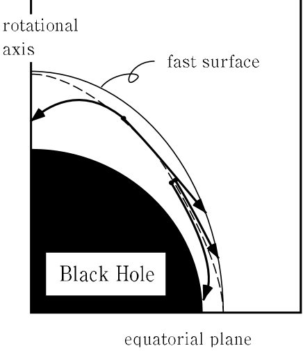
Figure 3: Schematic figure (side view) of a black hole magnetosphere. The thick solid curves denote the characteristics of equation (62). The fast-magnetosonic separatrix surface is denoted by the dashed line. The magnetic field lines are not drawn in order to avoid complication. The super-fast region is very thin in the magnetically dominated limit; however, the width of this region is exaggerated.

Since fluid obtains most of its perturbation energy from the electromagnetic field at the maximum amplitude surface, $\xi=0$, most of the fluid’s disturbance propagates almost along the separatrix (i.e., the maximum amplitude surface) and at last deviates inwards or outwards. In other words, meridional propagation is essential to examine the spatial structure of fluid disturbance near to the fast-surface. As a result of the deviation of waves, $1/{\rm Im}(\delta)$, and hence fluid amplitude, rapidly decreases with $\theta$ as indicated in Fig. 2 for a prolate shape of the fast-surface. We can quantitatively understand this behavior by considering an approximate solution

$$\rm{Im}(\delta)\propto\exp\left(-\frac{1}{2}\int_{0}^{\theta}\left[\frac{d{x}_{\rm F}}{d\theta}\right]d\theta\right),$$ (64)

which is applicable when $d^{2}{x}_{\rm F}/d\theta^{2}\approx 0$. Equation (64) indicates that $\rm{Im}(\delta)$ decreases exponentially as $\theta$ decreases.

Let us finally consider the relation of amplitude among various perturbed quantities. Combining equations presented in the last section, we obtain near to the fast-point

$$\frac{e_{r}}{E_{\theta}/M},\frac{b_{\theta}}{B^{r}},u^{\theta}\approx\sqrt{\frac{\mu}{E}}u^{r}\ll u^{r}$$ (65)

in order of magnitude because of $k_{\perp}\approx\sqrt{E/\mu}k_{r*}$. Other electromagnetic quantities have much smaller amplitude near to the fast-surface. It is interesting to note that the equipartition of energy ($[e_{r}]^{2}\approx\mu n[u^{r}]^{2}$) is achieved near to the fast-surface, although the perturbation energy is supplied mainly in the form of electromagnetic disturbances ($[e_{r}]^{2}\approx[E/\mu]\mu n[u^{r}]^{2}\gg\mu n[u^{r}]^{2}$) far from the horizon, In other words, a lot of perturbation energy is deposited from the electromagnetic field to the fluid during the infall as a result of effective MHD interactions. In a realistic magnetically dominated black hole magnetosphere, the fluid becomes highly variable ($[u^{r}]^{2}\approx[U^{r}]^{2}$) near to the fast-surface for a very small input of perturbation energy ($[e_{r}]^{2}\approx[\mu/E][E_{\theta}/M]^{2}$) from the surroundings. The existence of the horizon is essential to make the fluid be highly variable near to the fast-surface (PaperI, and II). If the fast-surface is located far from the hole, fluid quantities does not become highly variable.

So far, we have derived the following conclusions: (1) The fluid quantities become highly variable near to the fast-surface owing to MHD interactions near the horizon. (2) Their amplitude is a peaking function at the separatrix surface located slightly inside of the fast-surface. This is because a large-amplitude fluid disturbance propagates along the separatrix as a outgoing fast-wave. (3) For prolate shape of the fast-surface, for instance, The fast-waves that propagate towards the equator can reach the fast-surface and escape to the sub-fast region. These results drive us to the question how these fast-waves propagate in the sub-fast regions. In the next section, we will be concerned with this issue.

4 Wave propagation in sub-fast region

4.1 Geometrical optics in relativistic accretion

As we have seen, meridional wavelength is much less than the radius of curvature near to the fast surface. It follows that the propagation of wave packets of fast-magnetosonic mode follows the laws of geometric optics. In geometrical optics, the nature of the second-order partial differential equations describing the propagation can be well studied by the characteristic hypersurfaces of the system. The characteristic hypersurfaces, which play the role of wave fronts, can be expressed by a surface of $\psi(x^{\mu})=$ constant, where $\psi$ satisfies the following eikonal equation in the cold limit (Lichnerowicz 1967; see also Takahashi et al. 1990 for sound waves):

$$H\equiv s^{\alpha\beta}\psi_{,\alpha}\psi_{,\beta}=0,$$ (66)

where $s^{\alpha\beta}$ is defined by

$$s^{\alpha\beta}\equiv g^{\alpha\beta}+\frac{{U^{\alpha}}{U^{\beta}}}{U_{\rm FM}^{2}};$$ (67)

$U_{\rm FM}$ is the fast-magnetosonic speed in $d\tau$-basis and is defined by

$$U_{\rm FM}^{2} \equiv \frac{KB_{\rm p}^{2}+B_{\phi}^{2}/\rho_{\rm w}{}^{2}}{4\pi\mu n}$$ (68)

$$= \frac{K_{\rm I}-K}{4\pi\mu\eta}\frac{B^{r}}{U^{r}}.$$

The first term in equation (67) describes the influence of the gravitational field, while the second term that of cold, relativistic magnetohydrodynamic flows. If we were to replace $\psi_{,\alpha}$ with $k_{\alpha}$, we would obtain the dispersion relation for the fast-magnetosonic mode,

$$\left(U^{\mu}k_{\mu}\right)^{2}+U_{\rm FM}^{2}k^{\mu}k_{\mu}=0.$$ (69)

Instead of solving the partial differential equation (66), we can investigate the trajectories of wave packets by solving a set of the following ordinary differential equations:

$$\frac{dx^{\alpha}}{d\lambda} = \frac{\partial H(x^{\beta},p_{\beta})}{\partial p_{\alpha}},$$ (70)

$$\frac{dp_{\alpha}}{d\lambda} = -\frac{\partial H(x^{\beta},p_{\beta})}{\partial x^{\alpha}},$$ (71)

where $\lambda$ is the parameter along a ray path. Since the Hamiltonian $H$ contains neither $t$ nor $\phi$, both wave frequency $\omega=P_{t}$ and azimuthal wave number $m=-P_{\phi}$ are conserved along a ray path.

The unperturbed fluid’s velocity field, on which the wave packets propagate, must be solved consistently with the equations of motion. First, the definition of proper time gives the poloidal wind equation

$$g_{rr}(U^{r})^{2}+1=-\frac{g_{\phi\phi}(U_{t})^{2}-2g_{t\phi}U_{t}U_{\phi}+g_{tt}(U_{t})^{2}}{\rho_{\rm w}{}^{2}}$$ (72)

Secondly, combining the unperturbed continuity equation, Maxwell equations, and the frozen-in conditions with equations (5) and (6), we obtain (Camenzind 1986b)

$$\mu U_{t} = \frac{(g_{tt}+g_{t\phi}\Omega_{\rm F})\epsilon-{\cal M}^{2}E}{K-{\cal M}^{2}},$$ (73)

$$\mu U_{\phi} = \frac{(g_{t\phi}+g_{\phi\phi}\Omega_{\rm F})\epsilon+{\cal M}^{2}L}{K-{\cal M}^{2}},$$ (74)

where the Alfv$\acute{\rm e}$nic Mach number ${\cal M}$ is defined as

$${\cal M}^{2}\equiv\frac{4\pi\mu\eta^{2}}{n}=\frac{4\pi\mu\eta}{B^{r}}U^{r}.$$ (75)

We assume an appropriate functional form for $B^{r}$ instead of solving the unperturbed trans-field equation.

These three equations, (72)-(74), together with (75), give the fluid’s velocity field ($U_{t}$, $U^{r}$, $-U_{\phi}$) on the poloidal plane. We assume that the accretion along each radial field line starts from the point at which $K$ becomes 0.55. This condition defines a nearly spherical (but somewhat oblate) injection surface of accretion at ${r}_{\rm I}\approx 5M$ for a mildly rotating hole ($a\approx 0.5M$). We suppose that there is no flow of plasmas outside of the injection surface. This assumption alters the propagation of the fast waves negligibly, because plasma flows in the region $5M<r<10M$ is non-relativistic, whereas the fast-magnetosonic speed in $dt$-basis is slightly smaller than that of light. We further assume that the energy density of the magnetic field is nine times larger than that of the fluid’s rest-mass in the sense that $E/(\mu\sin^{2}\theta)=-10$.

In this section, we trace the ray paths of the fast-magnetosonic wave packets radiated meridionally with momentum $|k_{\perp}|\approx\sqrt{E/\mu}\,|k_{r*}|$ from the fast-magnetosonic surface rather than radiated spherically (i.e., in all directions), by solving equations (70) and (71) in the magnetically dominated accretion described by equations (72)-(74).

4.2 Collimation of MHD waves

Let us first demonstrate typical results when the fast-magnetosonic speed, $U_{\rm FM}$ is slower in polar regions than in equatorial regions. Such a distribution of $U_{\rm FM}$ will be realized when $|B^{r}|$ is smaller in the polar regions. A good example of such a magnetic field was presented by Blandford & Znajek (1977); they solved the vacuum Maxwell equations in a Kerr space time and derived a split monopole field, $B^{r}=B_{0}\sin\theta+O(a^{2}/M^{2})$ for a distribution of a toroidal surface current density of $I\propto r^{-2}$. Specifically, we assume that $B^{r}/(4\pi\mu\eta)=(-E/\mu\sin^{2}\theta)(1-0.8\cos\theta)^{2}$ in this paper and calculate $U_{\rm FM}$ along a ray path by solving equation (68). In this case, $|\eta|$ becomes larger in the polar regions; therefore, the distribution of the fast-surface (Paper 1)

$$\frac{{r}_{\rm F}-{r}_{\rm H}}{{r}_{\rm H}}=\frac{\pi\Sigma_{\rm H}{}^{2}}{({r}_{\rm H}-M)M{r}_{\rm H}}A_{1}(\theta)\mu\eta$$ (76)

becomes prolate. Here, the function $A_{1}(\theta)$ is of order of unity and has a weak dependence on $\theta$ as

$$A_{1}\equiv\frac{\sqrt{K_{\rm I}-K}}{(1-a\Omega_{\rm H}\sin^{2}\theta)(1-a\Omega_{\rm F}\sin^{2}\theta)^{3}W^{3}},$$ (77)

where $W$ is a function of $\theta$ and of order of unity. For radial distribution of field lines, $W^{2}$ becomes

$$W^{2}\equiv 1+\frac{2a{r}_{\rm H}(\Omega_{\rm H}-\Omega_{\rm F})\sin^{2}\theta}{({r}_{\rm H}-M)(1-a\Omega_{\rm H}\sin^{2}\theta)(1-a\Omega_{\rm F}\sin^{2}\theta)}.$$ (78)

The information on the injection point of accretion appears only through $K_{\rm I}=0.55$.

Examples of ray paths of axisymmetric waves ($m=0$) are presented in Fig. 4. All the wave packets are radiated from $0<\theta<\pi/2$ (the first quadrant) in this figure. Even though the wave packets have no angular momenta ($m=0$), they have non-zero angular velocities because of the space-time dragging and the rotational motion of the accretion flow. Therefore, the ray paths are projected on their instantaneous poloidal plane and are depicted in the figure. Since $U_{\rm FM}$ is smaller in higher latitudes, the fast-surface becomes prolate; thus the waves that propagate towards the equator can escape into the sub-fast regions. As a result, the wave packets radiated from the first quadrant propagate clockwise as depicted in this figure. Because of the accretion, waves are pushed backwards to the hole and revolve around it. The heavy solid line on the equatorial plane denotes a dense disk which possibly resides around an active bole. If a wave packet collides with the disk, it will be totally absorbed to heat the plasma there.

Figure 4: Side view of ray paths of fast-magnetosonic wave packets in a magnetically dominated accretion flow around a mildly rotating black hole of $a=0.5M$. Ray paths are radiated meridionally from the fast-surface every $5$ degrees in the first quadrant: Solid curves denote ray paths radiated from the high latitudes ($5^{\circ}$, $10^{\circ}$, $15^{\circ}$, $20^{\circ}$, $25^{\circ}$, and $30^{\circ}$). Dashed curves from the middle latitudes ($35^{\circ}$, $40^{\circ}$, $45^{\circ}$, $50^{\circ}$, $55^{\circ}$, and $60^{\circ}$ degrees), while dotted curves from the low latitudes ($65^{\circ}$, $70^{\circ}$, $75^{\circ}$, $80^{\circ}$, and $85^{\circ}$). Fast-magnetosonic speed is lower in the polar regions than in the equatorial regions. As a result, fast waves collimate towards the rotation axis.

Figure 5: Side view of the ray paths of non-axisymmetric mode. The solid lines denote $m=2$ mode, while the dashed, dash-dotted, dotted, and dash-dot-dot-dotted lines denote $m=4$, $m=6$, $m=8$ $m=10$ modes, respectively. Waves propagating in the right hemisphere are radiated meridionally at $\theta=30^{\circ}$, whereas those in the left one are radiated at $\theta=-45^{\circ}$.

Figure 6: The same figure as Fig. 4; however, the fast-magnetosonic speed is slower in the equatorial regions than in the polar regions. As a result, fast waves are bent towards the equatorial plane to form a focal ring.

This figure indicates that most of the wave packets which are radiated meridionally from the fast-surface, collimate into the polar regions where $U_{\rm FM}$ is small. Qualitatively the same results are obtained for non-axisymmetric waves. In Fig. 5, $m=2,4,6,8,10$ waves are depicted. Ray paths in the first and the fourth quadrant originate at $\theta=30^{\circ}$, whereas those in the second and the third quadrant originate at $\theta=-45^{\circ}$ (in the second quadrant). Wave packets with negative angular momentum ($m<0$) are not drawn, because they are soon swallowed by the hole. As the figure indicates, non-axisymmetric waves cannot reach the rotational axis because of their non-zero angular momenta; therefore, the tendency of collimation is somewhat weakened compared with $m=0$ modes depicted in Fig.  4.

In section 6, we discuss that the collimated waves may experience resonance and mode-convert itself into electromagnetic waves to result in a particle acceleration by non-linear interactions. Before we come to this issue, one more point must be clarified: if $U_{\rm FM}$ are larger in the polar regions than in the equatorial regions, ray paths must be bent towards the equatorial plane. We examine briefly this case in the next subsection.

4.3 Formation of a focal ring

We demonstrate here typical results when the fast-magnetosonic speed, $U_{\rm FM}$, is faster in the polar regions than in the equatorial regions. In this case, the distribution of the fast-surface becomes oblate. Examples of ray paths for axisymmetric modes ($m=0$) are presented in Fig. 6. All the wave packets are radiated from $0<\theta<\pi/2$ (the first quadrant) in this figure. Since the fast-surface is oblate, the wave packets that propagate initially towards the rotational axis can escape into the sub-fast regions. Therefore, the waves propagate counterclockwise.

This figure indicates that most of the wave packets bent towards the equatorial disk to form a focal ring of radius $\sim 5M$ and do not collimate towards the rotational axis. For non-axisymmetric waves, this tendency is strengthened because of their non-zero angular momenta.

5 Discussion

We have demonstrated that the magnetically dominated plasma accretion becomes highly variable near to the fast surface located close to the horizon and that such fluid’s disturbance propagates as a fast-magnetosonic wave and collimates towards the rotational axis (especially for an axisymmetric mode) when the fast-magnetosonic speed is slower in the polar regions than in the equatorial regions. In the framework of MHD, the collimated fast waves will not cause interesting phenomena such as particle acceleration, even in nonlinear regimes. However, if we take the effects of plasma oscillation and cyclotron motion of particles into account, interesting results such as particle acceleration at a resonant point may be obtained (Holcomb and Tajima 1992; Daniel and Tajima 1977). For this reason, we consider in this section a plasma wave in a pure electron-positron plasma (for observational and theoretical discussion on the existence of electron-positron plasmas in AGN jets, see Ghisellini et al. 1992; Morrison et al. 1992; Xie et al. 1995; Reynolds et al. 1996).

As Fig. 4 indicates, wave vectors ($\vec{k}$) of collimated fast waves are nearly parallel to the magnetic field ($\vec{B}$), of which poloidal components dominate the toroidal one near the rotational axis. It is, therefore, possible to regard that the collimated waves propagate as shear Alfvén waves.

In fact, a shear Alfvén mode is one of the two primary modes in a pure electron-positron plasma when $\vec{k}\parallel\vec{B}$. The other mode is an electromagnetic mode. Their dispersion relation is given by

$$k^{2}=(k_{r})^{2}=\frac{\omega^{2}(\omega^{2}-\Omega_{\rm e}{}^{2}-2\omega_{\rm p}{}^{2})}{c^{2}(\omega^{2}-\Omega_{\rm e}{}^{2})},$$ (79)

where the plasma and cyclotron frequencies are defined by

$$\omega_{\rm p} \equiv \sqrt{4\pi ne^{2}/m_{\rm e}},$$ (80)

$$\Omega_{\rm e} \equiv \frac{eB^{r}}{m_{\rm e}c}.$$ (81)

If we would set $\Omega_{\rm e}\gg\omega,\ \omega_{\rm p}$, we could recover the dispersion relation of an usual Alfvén mode, which is identical with that of a fast-magnetosonic mode when $\vec{k}\parallel\vec{B}$ in a cold plasma. Exactly speaking, we must take account of geometrical correction due to hole’s gravity in the definitions (80) and (81); however, at the height where $r>10M$, such effects become negligible.

From the dispersion relation (79), it follows that a shear Alfvén mode exists for frequencies less than $\Omega_{\rm e}$ (the resonance frequency), while an electromagnetic mode exists for frequencies greater than $\sqrt{\Omega_{\rm e}{}^{2}+2\omega_{\rm P}}$ (the cut-off frequency). In a realistic black hole magnetosphere, $\Omega_{\rm e}$ is a decreasing functions of distance ($r$) from the hole, because $B^{r}$ decreases with $r$.

It is important to note that the point of cut-off is located slightly outside of the point of resonance in a magnetically dominated magnetosphere ($m_{\rm e}n_{\rm e}c^{2}\ll B^{2}/8\pi$). Therefore, we can depict the following scenario according to [Budden (1961)]: A shear Alfvén wave packet is injected outwards by the mechanism described in the preceding sections. As the wave approaches the point of resonance (a magnetic beach), it increases the amplitude owing to a nonlinear effect. After reaching the point of resonance, it evanesces through the thin evanescent region to transmit as an electromagnetic wave above the point of cut-off.

When the amplitude of injected shear Alfvén wave is high and nonlinear effects become important, the wave may capture many particles to hide the singularity. In this case, they continue to propagate as an Alfvén mode after passing the ‘singularity’ owing to the so-called self-induced tunneling (e.g., McCall, Hahn 1969). As a result, the trapped particles may be accelerated through long distances to become relativistic. According to the nonlinear simulations performed by Daniel and Tajima (1977), who adopted a very thin evanescent layer corresponding to a magnetic dominance of $B^{2}/8\pi\sim 9n_{\rm e}m_{\rm e}c^{2}$, particle acceleration up to energies of $8m_{\rm e}c^{2}$ can be realized if the injected wave is highly nonlinear. On these grounds, it seems reasonable to conclude that the process of wave amplification and collimated demonstrated in this paper triggers initial acceleration of jet due to a cyclotron resonance in an electron-positron plasma.