Two Dimensional Galaxy Image Decomposition

Abstract

We propose a two dimensional galaxy fitting algorithm to extract parameters of the bulge, disk, and a central point source from broad band images of galaxies. We use a set of realistic galaxy parameters to construct a large number of model galaxy images which we then use as input to our galaxy fitting program to test it. We find that our approach recovers all structural parameters to a fair degree of accuracy. We elucidate our procedures by extracting parameters for 3 real galaxies – NGC 661, NGC 1381, and NGC 1427.

1 Introduction

The luminosity profile of a typical spiral or S0 galaxy most often contains two components, a spheroidal bulge and a circular disk. If the galaxy possesses an active nucleus, then a high central point intensity may also be present. The projected bulge intensity profile is usually represented by an $r^{1/4}$ law (de Vaucouleurs , 1948), where $r$ is the distance along the major axis, say. For disks an exponential law is frequently used (Freeman, 1970). These profiles are entirely empirical, and have not been derived from a formal physical theory. However, numerical simulations in simplified situations such as those by van Albada (1982) have been able to recreate $r^{1/4}$ profiles for the bulge.

The photometric decomposition of galaxies into bulge and disk and the extraction of the parameters characterizing these components has been approached in a number of ways. Early attempts at such decomposition assumed that the disk would be the dominant component in the outer regions of galaxies and that the bulge would dominate the inner regions. Disk and bulge parameters were extracted by fitting for each component separately in the region in which it was dominant by authors such as Kormendy (1977) and Burnstein (1979). Schombert and Bothun (1987) employed such a technique for initial estimation of bulge and disk parameters of simulated galaxy profiles, with standard laws describing the bulge and the disk with simulated noise. These parameters were then used as initial input to a $\chi^{2}$ fitting procedure. Tests on simulated profiles indicated good recovery of both bulge and disk parameters. For a review of various 1-D decomposition techniques see Simien (1989). The conventional technique of fitting standard laws to a 1-D intensity profiles extracted from galaxy images was critically examined by Knapen and van der Kruit (1991). They found that even for the same galaxy different authors derive disk scale length values with a high average scatter of 23%. Such large uncertainty in the extracted structural parameters is a hindrance in the study of structure, formation and evolution of the bulge and disk of galaxies. Accurate, reliable determination of bulge and disk parameters is a prerequisite for differentiating between competing galaxy formation and evolution models. The conventional one dimensional technique is also limited because it assumes 1-D image profiles can be uniquely extracted from galaxy images. This is not possible if a strong but highly inclined disk is present.

A two dimensional technique which uses the entire galaxy image rather than a major axis profile overcomes this difficulty. Such a technique was proposed by Byun and Freeman (1995), henceforth BF95. A similar approach was used by R. S. de Jong to extract parameters for a sample of 86 face on disc dominated galaxies (de Jong, 1996), henceforth DJ96.

In this paper, we describe a 2-D decomposition technique similar to the one employed in BF95. Extending this work, we fit for a central point source in addition to a bulge and a disk. In addition, our method takes into account the effects of convolution with a PSF and of photon shot noise from sky background and the galaxy. We believe that PSF convolution will significantly affect parameters, especially those of the bulge. We also study the effects of the convolution on the extraction of a point source. We also try to quantify effects of other features such as foreground stars on parameter extraction. We illustrate the efficacy of our methods by extracting bulge and disk parameters for three galaxies in two different filters. We also briefly discuss reliability of error bars on parameters extracted.

In the next section, we describe our method of constructing artificial galaxy images as tests for our bulge–disk–point decomposition procedure. Section 3 describes the decomposition procedure. Section 4 is a detailed analysis of the testing we performed on it, using artificial galaxy images.. Section 5 is a description of application of the technique to three real galaxies. Section 6 contains a discussion about error bars on the parameters extracted. Section 7 contains the conclusions.

2 Simulation of Galaxy Images

In order to test the bulge and disk decomposition procedure, we have developed a galaxy image simulation code to generate images closely resembling those obtained using CCD detectors on optical telescopes. Using the code it is possible to simulate a CCD image of a galaxy with an arbitrary bulge, disk and point at an arbitrary position and orientation on the CCD. The image can be convolved with a given circular or elliptic PSF and Poisson noise can be added if required. Stars can be introduced into the image at random positions and additional features of galaxies such as absorbing dust lanes can be added. All parameters used by the program can be easily modified by the user through a parameter file.

Galaxy profiles are the projections of three dimensional luminosity profiles onto the plane of the sky. The disk is inherently circular, so it projects as an ellipse. The inclination angle of the disk with respect to the plane of the sky completely determines the ellipticity of the disk in the image. Bulges, taken to be triaxial ellipsoids in the general case, also project as ellipses. The ellipticity of the bulge does not reach such high values as the disk. For a triaxial ellipsoid with major axis $a$, minor axis $b$, and an intermediate axis $c$, the highest possible ellipticity will be $1-b/c$. Therefore the projected galaxy shows elliptical bulge isophotes and in many cases – more elliptical disk isophotes.

For an arbitrary point on the image plane, intensity contribution comes from the bulge and the disk, and depends on their respective central intensities, ellipticities and scale lengths. Near the galaxy center there is an additional contribution from the point source, if one is present.

In our galaxy simulation, the projected bulge component is represented by the $r^{1/4}$ de Vaucouleurs law with effective (half light) radius $r_{e}$ (which is the radius within which half the total light of the galaxy is contained), intensity at the half light radius $I_{e}$ and a constant ellipticity $e_{b}=1-\rm(minor\ axis\ length/major\ axis\ length)$:

$$I_{bulge}(x,y) = I_{e}e^{-7.67[(r_{bulge}/r_{e})^{1/4}-1]},$$ (1)

$$r_{bulge} = \sqrt{x^{2}+y^{2}/(1-e_{b})^{2}},$$

where $x$ and $y$ are the distances from the center along the major and minor axis respectively.

The projected disk is represented by an exponential distribution with central intensity $I_{s}$, scale length $r_{s}$ and a constant ellipticity $e_{d}$,

$$I_{disk}(x,y) = I_{s}e^{-r_{disk}/r_{s}},$$ (2)

$$r_{disk} = \sqrt{x^{2}+y^{2}/(1-e_{d})^{2}}.$$

The disk is inherently circular. The ellipticity of the disk in the image is due to projection effects alone and is given by:

$$e_{d} = 1-\cos(i)$$ (3)

where $i$ is the angle of inclination of the circular disk with the image plane. Finally, the point source is represented by an intensity added to the central pixel of the galaxy prior to convolution.

We use these empirical laws for the bulge and the disk keeping in mind that they do not satisfactorily describe all galaxies. Features such as stars can be added if required. Stars are added at random positions as intensities at a single pixel prior to convolution with the PSF. The convolution with the PSF is performed in the Fourier domain. For adding photon shot noise, a constant sky background is added to every pixel. The resultant count in each pixel (which includes intensity from the galaxy as well as the sky background) is multiplied by the gain (electrons/ADU). A random Poisson deviate about this value is obtained. The deviate is then divided by the gain and the background is subtracted out.

The program takes about 15 seconds to generate a galaxy image, when running on a Sparcstation 10 for a 256 $\times$ 256 pixel image. A copy of this code (written entirely in ANSI C) is available upon request.

3 2-D Decomposition Technique

3.1 Building The Model

The model to be fit is constructed using the same procedure as the simulated images described in the previous section, except that features of the image that are not contributed by the galaxy such as stars and Poisson noise are not added.

3.2 The Decomposition Procedure

To effect the decomposition, we attempt to iteratively minimize the difference between our model and the observed galaxy (or a simulated one), as measured by a $\chi^{2}$ value. For each pixel the observed galaxy counts are compared with those predicted by the test model. Each pixel is weighted with the variance of its associated intensity as determined by photon shot noise of the combined sky and galaxy counts at that pixel. Photon shot noise obeys Poisson statistics and so the variance is equal to the intensity value. Hence:

$$\chi_{\nu}^{\,2}={1\over\nu}\sum_{i,j}{[I_{model}(i,j)-I_{obs}(i,j)]^{2}\over I_{obs}(i,j)},$$ (4)

where $i,j$ range over the whole image, $\nu=N-$ (number of fitted parameters) is the number of degrees of freedom with $N$ being the number of pixels in the image involved in the fit, and $I_{obs}$ is assumed to be greater than zero in all cases.

CCD images of galaxies contain features such as foreground stars and bad pixels that may contaminate the decomposition procedure. We take care to block out bad pixels and visible foreground stars before commencing decomposition.

For real galaxies, our decomposition program assumes that pixel values $I$ represent real photon counts. If the image has been renormalized in any way (divided by the exposure time for example), the extracted $\chi^{2}$ value should be multiplied by the appropriate factor to account for that normalization.

Seven fitting parameters are used in our scheme. These are $I_{e},I_{s},r_{e},r_{s},$ $e_{b},e_{d},$ and a central point source intensity $I_{p}$. The first 4 parameters were used by Schombert and Bothun (1987), and the first six were used by the authors of BF95 and DJ96. We have added capability in our code to fit for position angle and a constant background. During our preprocessing we estimate the background carefully and subtract it out. Where it is possible in real cases, fitting for sky background is not required.

The minimization uses MINUIT 94.1, a multidimensional minimization package from CERN, written in standard FORTRAN 77. MINUIT allows the user to set the initial value, the resolution, and the upper and lower limits of any parameter in the function to be minimized. Values of one or more parameters can be kept fixed during a run. MINUIT has several strategies to perform the minimization. Our method of choice is MIGRAD, a stable variation of the Davidon–Fletcher–Powell variable metric algorithm. It calls the user function (in our case $\chi_{\nu}^{\,2}$) iteratively, adjusting the parameters until certain criteria for a minimum are met. Our code typically takes 0.1 seconds per iteration on a SGI Indigo 2 workstation, when working on a 64 $\times$ 64 pixel galaxy image. On a slower Sparcstation 10, time taken increases by a factor of about 1.5. Since we are using fast Fourier transforms to convolve the model with a gaussian PSF, the execution time can be expected to scale as $N\log N$, with $N$ the total number of pixels in the image. We do find that execution time scales almost linearly with the number of pixels in the image. About 1000 iterations are required for convergence criteria to be satisfied when all 7 parameters are kept free, so a typical run takes less than two minutes. Computation time is reduced as the number of free parameters is reduced.

A copy of this code (written mostly in ANSI C with some optional display routines in IDL) is available upon request.

4 Reliability of Galaxy Image Decomposition

We conducted elaborate tests of the effectiveness of the program in extracting parameters under different input conditions. The tests of error in PSF measurements serve as warnings against claiming too much accuracy in the extraction of a point without very accurate measurements of the PSF.

4.1 Large-Scale Testing under Idealized Conditions

To test the accuracy and reliability of our algorithm, we constructed a wide range of model galaxies with idealized bulge and disk components. Images of 500 model galaxies were generated by random uniform selection of intensities, scale lengths and ellipticities. The ranges we used for each of the parameters are,

1. for the bulge

   $$18< \mu_{\em eff} <24\ {\rm mag\ arcsec^{-2}},$$

   $$3< r_{e} <30\ {\rm pixels},$$

   $$0.0< e_{b} <0.4,$$

2. and for the disk

   $$15.5< \mu_{s} <21.5\ {\rm mag\ arcsec^{-2}},$$

   $$3< r_{s} <30\ {\rm pixels},$$

   $$0< e_{d} <0.9.$$

The ranges chosen for the parameters encompass most values encountered in real galaxies, and the intensities were chosen to correspond to the above magnitudes using photometric data on a 1m class telescope. Note that we fit in intensity space, not magnitude space, so the values were distributed approximately uniformly in intensity space. The galaxies generated by the galaxy simulation program were then used as input to the bulge disk decomposition program. We studied how accurate and reliable the decomposition program is in recovering the input parameters.

We place no additional relative constraints on permissible parameter values such as those used in BF95. We find that the $\chi_{\nu}^{\,2}$ for the fits is worse than 2 in only 25 cases out of 500, giving a 5% failure rate. These failures are caused by the presence in parameter space of local minima close to the starting values given to MINUIT, or by one or more parameters hitting their limits, causing the gradient-driven minimization routine to fail. It is possible to completely eliminate such failure by changing the initial value and constraining the range of parameters around the expected value. Such a procedure cannot be adopted while working with real galaxies as it is not possible to constrain the parameters a priori. We find that a $\chi_{\nu}^{\,2}<2$ almost always corresponds to good recovery of input parameters, and a $\chi_{\nu}^{\,2}>2$ always corresponds to poor recovery of input parameters. Poor recovery of one parameter almost always implies poor recovery of all other parameters, and a high value of $\chi_{\nu}^{\,2}$. In the instances of poor recovery deviations from true values for different parameters are not correlated, which is consistent with the high values of $\chi_{\nu}^{\,2}$ obtained for them.

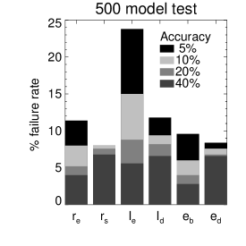
Figure 1: Failure level in 500 point test. The Y axis shows percentage of cases in which the program fails to recover the parameter indicated on the X axis at a level indicated by the shading (see text)

The parameter errors are summarized in Fig. 1. There is a column for each parameter, with the shading indicating which failure level the bar represents. For example, for 5% of models, the program failed to extract the bulge scale length with an accuracy of better than 20%, and for 7% it failed to extract the same parameter with an accuracy of better then 10%. Accuracy is defined here as the the difference of the input parameter and the recovered parameter, divided by the input parameter and expressed as a percentage.

Figure 2: Scatter plots of extracted versus input parameters. Parameters extracted with $\chi_{\nu}^{\,2}>2$ are indicated by a $\times$

From Fig. 1 we see that all input parameters except bulge intensity are extracted with less than 10% error in over 90% of the test cases. The bulge intensity seems to have been extracted less accurately than the other quantities. The extracted versus input data have been plotted in Fig.  2, with points having $\chi_{\nu}^{\,2}>2$ marked with a $\times$. Note that the points with a bad fit generally lie far away from the line on which the input value equals the extracted value. Most of the remaining points (those with $\chi_{\nu}^{\,2}<2$) plotted on these graphs are tightly grouped along this line. There is no systematic trend in the deviation of extracted parameters from their true value for any of the parameters plotted. The scatter plot in Fig. 2 is tighter than a similar plot presented in BF95.

In a real situation, one would not be running blind, and if minimization failed with one set of parameters, one would use different starting values and try again. It should be noted that failure in recovering parameters is easy to detect as it is always flagged by a high $\chi^{2}$ value. We conclude that for our test cases at least, the input parameters are recovered very well, and without systematic or significant deviations.

4.2 Tests of stability

We conducted a series of tests to determine how the program responds to deviations from the idealized conditions assumed in the previous section. We looked at some of the problems encountered when dealing with real images rather than simulated ones.

4.2.1 Effect of changing S/N ratio

The S/N ratio improves with increase in exposure time. We examined the image of the same simulated galaxy using pixel counts for a bright galaxy and sky background corresponding to exposure times ranging from about 5 seconds to 8 minutes on a 1   m class telescope. The exposure times (and hence the pixel counts) varied by a factor of 96 and S/N ratio by a factor of about 10 ($\simeq\sqrt{96}$). The background counts used were estimated from observations made on a 1m class telescope in the Cousins R filter. We expected that as S/N got better, the fit would improve and parameter recovery would get more accurate. We found that the accuracy of the extracted parameter values is strongly dependent on the exposure time only for very short exposures ($<$ 30 seconds) (Table LABEL:tab:sbyn). Peak counts of less than one thousand for galaxies are not very useful for the purpose of bulge disk decomposition.

Exp. time	$\chi_{\nu}^{\,2}$	Peak	Input	Extracted	% Error in
(sec)		Counts	$I_{e}$	$I_{e}$	$I_{e}$
5	1.00	302	4.17	6.4	53.0
15	1.00	914	12.5	11.1	8.9
30	1.02	1923	25	24.2	3.2
60	1.04	3665	50	51.2	2.4
120	1.07	7623	100	101	1.0
240	1.11	14826	200	202	1.0
480	1.14	29740	400	415	3.75

Table 1: Effect of changing exposure time on extraction of bulge intensity

It is seen that $\chi_{\nu}^{\,2}$ increases slowly but monotonically with exposure time. This is an artifact of the way sky background is used in the program creating the input galaxies. When simulating galaxies, background is added, Poisson noise is calculated using the intensity of both background and galaxy, and the background is subtracted out. Then, when the fitting program runs, it estimates the noise at each pixel as the square root of the number of counts at that pixel, but the actual noise is the square root of the sum of the number of counts and the background. This causes the points with low counts to be weighted more than they should be, (resulting in higher $\chi_{\nu}^{\,2}$) but the difference is small.

4.2.2 Effect of erroneous measurement of PSF

With real data it is often impossible, even if a large number of stars are used, to measure the PSF to an accuracy of better than about 5%. One reason is variation of the PSF in different regions of the CCD. Therefore, it is important to know how the fit will react to an over– or under–estimation of the PSF, and to an elliptical PSF. The value of the point source is expected to be affected the most because of errors in PSF estimation. If the bulge scale length $r_{e}$ is very small, then bulge parameters will also be seriously affected by an incorrect estimation of the PSF. We ran two separate tests, one with a circular PSF, overestimated or underestimated by up to 20%, and another where only one axis of the PSF changed by 20% while the other remained constant thereby generating elliptical PSFs. For the fitting we used a circular PSF with FWHM of 1 pixel in all the test cases.

Our simulated images are generated using a PSF with FWHM $\sigma_{image}$; this corresponds to the psf determined by seeing conditions in an actual observing situation. The psf used as input to the decomposition program has FWHM $\sigma_{fit}$. $\sigma_{image}/\sigma_{fit}\neq 1$ corresponds to the situation where an error is made in the estimation of $\sigma_{image}$ in an observing run. Here we are assuming that the psf is circular and the only error is in estimating its FWHM. When $\sigma_{image}/\sigma_{fit}<1$ the spreading of the image due to seeing is over estimated. The excess deconvolved intensity at the center seen by the decomposition program then causes it to generate a fictitious point source. The minimum value for the ratio we have used in the test is 0.8. At this ratio the value of the point is very high intensity of the fictitious point source is very high, as can be seen from Fig. 3. The bulge intensity is at its minimum value. The intensity of the fictitious point source decreases and that of the bulge increases continuously as $\sigma_{image}/\sigma_{fit}\rightarrow 1$ If the FWHM of the psf is underestimated, i.e. $\sigma_{image}/\sigma_{fit}>1$, the point intensity becomes negative.

The variation $\sigma_{image}/\sigma_{fit}$ did not affect the extracted disk scale length, which only once deviated by more than 1 pixel. The disk intensity increased with increasing input PSF, analogous to the increase in bulge intensity discussed above. The extracted bulge and point source intensities, and bulge radius, all vary systematically and approximately linearly with the error in PSF estimation. $\chi_{\nu}^{\,2}$, is very good in all cases, decreasing somewhat as the PSF gets to be closer to our estimate of 1. These results are plotted on the left panel of Fig. 3.

To see the effect of errors in determining the shape of the PSF, we generated galaxies with different elliptical PSFs. Such PSFs are observed, for example, if the plane of the CCD is inclined to the focal plane of the telescope. The decomposition program continued to use a fixed circular PSF. The sequence of image PSFs was generated by keeping one of the principal axis of the ellipses always equal to $\sigma_{fit}$, and varying the other principal axis so that ratio of the two changed from 0.8 to 1.2. The results of parameter extraction are plotted on the right panel of Fig. 3, as a function of $\sigma_{image}/\sigma_{fit}$, where the ratio is now taken along the changing principal axis.

When the PSFs used in the simulation as well as fitting are both circular, but unequal, the fitting procedure leads to a positive or negative fictitious point source. A good overall fit is obtained with $\chi_{\nu}^{\,2}$ close to unity in the latter case, i.e. when $\sigma_{image}/\sigma_{fit}>1$, because here the overall intensity at the centre remains small and best fit bulge parameters which give a good fit, together with the negative point source can be found. In the case of a positive point source, changed bulge parameters cannot compensate for the error in the PSF and the quality of the fit is diminished. In the case of the elliptical PSFs, $\chi_{\nu}^{\,2}$ is greater than unity on both sides of $\sigma_{image}/\sigma_{fit}=1$.

Bulge ellipticity, which was set to 0.1 in all simulated images, was extracted very well in the case of the circular PSF as it varied over its range of FWHM. When the PSF becomes elliptical, we expect the extracted ellipticity to increase as well, and it does, but only to 0.12 for the most elliptic PSF, which had ellipticity 0.2. The ellipticity close to the centre of the galaxy is of course wholly determined by the shape of the PSF, while further away, the effects on the extracted ellipticity are much smaller.

Figure 3: Effects of incorrect estimation of PSF’s on extracted parameters. The panels show changes in point intensity, bulge intensity and bulge scale length under a changing circular PSF (left panel) and a changing ellipticity of the PSF . The dashed lines indicate the values of input intensities, which were held constant. The Y–axis shows the corresponding fitted intensity. See the text for an explanation

4.2.3 Fitting in the presence of stars

We added upto 20 randomly positioned stars to a 128 $\times$ 128 pixel image, where the star brightnesses were clearly visible in a magnitude plot, and ran the program without blocking out the stars. The presence of the stars worsened the $\chi^{2}$ considerably but the extracted parameters were not affected in any significant or systematic way. Masking out the stars improved the $\chi^{2}$ to normal values ($\approx 1$), without affecting the accuracy of the parameter recovery.

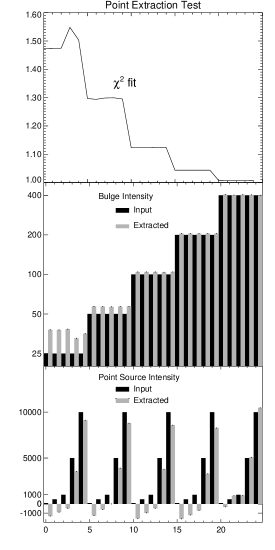
Figure 4: Results for test of point extraction in 25 runs. The top panel shows the $\chi_{\nu}^{\,2}$value. The bulge intensity increases after every 5 runs resulting in a steep drop in $\chi^{2}$. The middle panel shows 25 input values for bulge intensity and the corresponding recovered value adjacent to each other. Panel 3 shows input point source intensities for each run and the corresponding recovered value. See the text for an explanation.

4.3 Detecting a point source

We aim to model a point source in addition to the disk and bulge. The de Vaucouleurs bulge intensity has a very sharp peak near the center, so it should be easy for a point source to be swamped by the bulge unless it is very bright. The objective here is to find powerful sources, and we will not be concerned with the point source if its intensity is less than the bulge intensity over the central pixel. We looked at various strengths of the point relative to the bulge, by examining a uniform grid of $5\times 5$ values of point and bulge intensities, over which the bulge and point each varied by a factor of thirty. There was no detection of a fictitious point. Weak points were absorbed into the bulge, while strong points were extracted well, as shown in Fig. 4. For higher bulge intensities, the point intensity was extracted better, because higher S/N far from the center served to constrain the bulge intensity more precisely.

5 Fitting real galaxy images

The ultimate goal of this program is to extract parameters from a large sample of galaxies of different morphological types. Work on a large sample of spiral galaxies has been reported in RF96 and Byun, 1992. We report here parameters we extracted for two ellipticals and a lenticular galaxy. These galaxies were chosen to illustrate the algorithm’s ability to find the disk and bulge self-consistently. We selected the two ellipticals NGC 661 and NGC 1427 as simple tests, and one disk galaxy, NGC 1381, to illustrate how well the program is able to detect the disk. We expect to extract similar scale lengths in different bands and to get good fits ($\chi_{\nu}^{2}<2.0)$ in most cases.

5.1 Possible pitfalls

Going from fitting models to fitting real galaxies has several attendant dangers. Significant errors in the PSF can cause the detection of a fictitious point (Section 4.2.2). Since the PSF is never known exactly, any extraction of a point must be examined very carefully. Very close to the center, de Vaucouleurs law has not been shown to be correct, and there is evidence from HST data to the contrary (Byun et al 1996). Without very precise knowledge of the PSF, measuring systematic deviations from the law is not reasonable. Images are often normalized, averaged, or background subtracted in processing. Knowledge of the normalization used is required before we get an accurate estimate of the S/N ratio which is a prerequisite for determining the weighting function for our $\chi^{2}$ minimization.

5.2 NGC 661

NGC 661 has been classified as a possible cD galaxy with total magnitude in the B system $m_{\rm B}=12.88$ in the literature (RC3). We used images in two bands, V and R. We ran the processing twice in each band, once with the center masked out, and once with the center left unmasked. The results are shown in Table 2 and, for the particular of the $R$ band analysis with the central pixels included, in Figure 5. It is clear from panel C of the figure that the difference between the real and model galaxy profiles is very difficult to see with the eye. The difference becomes more discernible at large radii because of the poorer signal to noise ratio. The observed and model profiles appear irregular because we have plotted intensities along the major axis, rather than average isophotal intensities. The latter is usually done when considering results from 1-D profile fits.

We have included a bulge and a disk in our fits to NGC 661. It is seen from Table 2 that a weak disk, with total luminosity $\sim 4\%$ of the bulge, is detected. The disk has a scale length comparable to the FWHM of the PSF. It is therefore not possible to really distinguish between the disk and a point source. Moreover the detected disk simply could be an artifact of departures of the bulge profile, near the centre, from the de Vaucouleurs law form that we have assumed in our analysis. The ambiguity is evident from the large change in best fit disk scale length and intensity obtained in the $V$ band, in the cases with the central pixels masked and unmasked. Inclusion of a disk in the fit can affect the bulge parameters significantly as can be seen in the Table. Since the disk parameters cannot be trusted because of the reasons cited, the better alternative for a galaxy like NGC 661 is to fit a pure bulge profile. We shown the results of such a fit in Table 3. It is seen that the bulge parameters obtained in the two filters are equal to within the margin of error we found in parameter extraction for our simulated images in Section 4.1. The result obtained here is that the bulge scale lengths in the two filters are equal within errors expected in parameter extraction. The results shown in Table 2 are also consistent with this, but the bulge scale lengths obtained there are $\sim 25\%$ smaller. This example shows that features which are not clearly discernible given the PSF and the signal to noise ratio, should not be included in profile fits. Even though such features appear to be weak, they can significantly alter the fitted parameter values of the stronger features.

NGC 661: Bulge and Disk
$\chi^{2}$ $I_{e}$ $r_{e}$ $e_{b}$ $I_{d}$ $r_{s}$ $e_{d}$ $D/B$ R band 1.097 540.3 21.11 0.3042 7283 2.23 0.755 0.042 R band^† 1.075 522.6 21.45 0.3024 4681 2.701 0.7133 0.040 V band 1.378 381.6 19.63 0.3087 14078 0.0755 0.764 0 V band^† 1.092 638.2 14.91 0.2945 3988 2.374 0.1104 0.045

Table 2: Extracted parameters for NGC 661 in the R and V bands. $\dagger$ : Central pixels masked out.

NGC 661: Bulge only
$\chi^{2}$ $I_{e}$ $r_{e}$ $e_{b}$ R band 1.220 556.883 26.83 0.3315 V band 1.220 584.746 26.90 0.3195

Table 3: Extracted parameters for NGC 661 in the R band : Central pixels masked out

Figure 5: NGC 661 in the R band and our fit with the center unmasked. (a) is the 128 $\times$ 128 pixel image of the galaxy, with contours plotted at intervals of 1 magnitude. (b) is the contour of our extracted model, with the same contour levels. (c) is the profile along the major axis. When finished with the fitting, we step along the major axis, and produce a list of galaxy intensities and (PSF convolved) model, bulge and disk intensities at each point. On this plot the model is represented by a dashed line, and the real galaxy by a solid line. The difference between the real galaxy magnitude and the model is plotted just below. (d) shows the decomposition into bulge and disk, also convolved with the PSF.

5.3 NGC 1381

NGC 1381 is a galaxy of Hubble type SA0 and total magnitude in the B system $m_{\rm B}=12.60$ (RC3). We used images of this galaxy in the r,v, and g Gunn filters. Information about how this image was normalized was not available to us, so our estimate of $\chi_{\nu}^{\,2}$ should be taken as a relative measure only. It has a significant, highly elliptical disk, serving as a good test of our program’s ability to extract parameters when the isophotes are highly non-elliptical, and one-dimensional fitting programs are inapplicable (BF95).

Figure 3 shows the R band decomposition of the this galaxy. As in NGC 661, the difference between our model profile and the galaxy profile is very difficult to see with the eye, and is never more than 0.1 magnitude.

The bulge intensities are very similar both when the central pixels are masked out and when they are unmasked. The bulge scale length varies by $\sim 25\%$ in the v and r bands. The disk intensities are recovered consistently as well. We find that the disk scale length in Table 4 is very large compared to the size of the image, making the disk intensity approximately constant along its length, as is apparent from panel (d) of Fig 3. Since the disk ellipticity is high, we are looking at an edge on disk. This galaxy illustrates the capability of 2-D fitting to detect components with very high ellipticities. 1-D fitting that involves fitting ellipses to the image to generate ellipse profiles.

Bulge and disk ellipticities are extracted very consistently, with a maximum deviation of less than 4%.

NGC 1381
$\chi^{2}$ $I_{e}$ $r_{e}$ $e_{b}$ $I_{d}$ $r_{s}$ $e_{d}$ D/B Gunn g band 1.75 122.1 41.1 0.2885 294.4 357.5 0.9767 51.08 g band^† 1.419 117.4 42.72 0.2873 296.2 389.9 0.9775 58.85 v band 1.378 31.78 32.4 0.2808 47.93 255 0.9654 26.16 v band^† 1.363 48.04 24.76 0.2821 47.21 195.8 0.9585 22.28 r band 2.887 381.5 35.1 0.2816 828.2 236.5 0.9640 27.60 r band^† 2.774 513.5 28.72 0.2584 867.8 174.6 0.9496 17.49

Table 4: Extracted parameters for NGC 1381 in the Gunn g, v, and r bands. $\dagger$ : Central pixels masked out.

Figure 6: NGC 1381 in the R band and our fit with the center unmasked. For a description of the four panels see Fig. 5. The rectangular regions in the image were blocked out in preprocessing. Note that there are some deformed contours in the extreme upper right and lower left of the model image. These are an artifact of the convolution in Fourier space, and were masked out in the fit.

5.4 NGC 1427

This galaxy has been classified as a cD galaxy with total magnitude in the B system $m_{\rm B}=11.85$ (RC3). In this decomposition we only found a bulge. Since we had two images in the Gunn v and g filters and once in the r filter, we performed the decomposition separately on each image, to check the self-consistency of the algorithm. We find that it agrees well with itself where we have two images in the same wavelength, suggesting that the differences in scale length between different filters may have physical significance. The difference between scale lengths with and without masking of the central pixels is remarkable in the R band image. The intensities compensate for the difference, however so that the final $\chi_{\nu}^{\,2}$ are almost equal. In the R band, the disk is not wholly negligible unlike the other two bands where the $D/B$ ratio is extremely small. This is, however, a small perturbation on the bulge, as the bulge intensity is greater than that of the disk out to a large radius (about 40 pixels), and it is doubtful, but possible, that there is physical significance to this disk in the R band. The extracted bulge ellipticity is almost constant in all filters. However the extracted disk ellipticities show quite a wide scatter. This is not surprising considering that the disk is very weak and our estimate of the image PSF is only approximate.

NGC 1427
$\chi^{2}$ $I_{e}$ $r_{e}$ $e_{b}$ $I_{d}$ $r_{s}$ $e_{d}$ D/B g band (1) 2.218 109.3 46.67 0.3008 -1516 0.5579 0.9963 0.00 g band (1)^† 1.974 83.39 56.97 0.2948 108149 1.2184 0.8906 0.16 g band (2) 1.660 169.1 46.15 0.2822 4204 1.9594 0.5199 0.01 g band (2)^† 1.401 271.5 38.48 0.3193 -1976 7.6429 0.4728 -0.01 v band (1) 1.363 23.09 46.69 0.2819 -3775 0.451 0.1435 0.00 v band (1)^† 1.363 22.51 47.34 0.2784 1.448 175.9 0.9005 0.25 v band (2) 1.416 34.14 49.84 0.2750 -49330 0.1935 0.0777 0.00 v band (2)^† 1.413 32.58 51.64 0.2748 5.931 2465 0.7326 116.14 r band 1.306 423.50 27.80 0.2502 495.8 43.865 0.4034 0.82 r band^† 1.334 187.68 54.68 0.2680 130.02 71.213 0.5827 0.33

Table 5: Extracted parameters for NGC 1427 in the Gunn g, v, and r bands. Disk is much like either a point source or background in g and v bands. Two images each in g and v and one image in the r band was used. $\dagger$ : Central pixels masked out

Figure 7: NGC 1427 in the R band and our fit with the center unmasked. For a description of the 4 panels see Fig. 5.

6 Error estimation

In minimization problems, two methods are commonly employed for parameter error estimation. The first is to estimate the error from the second derivative of the function being minimized with respect to the parameter under consideration. The second is to gradually move away from the the minima until a predetermined $\chi^{2}$ is exceeded. The second method will work for a single parameter fit irrespective of whether the minima is parabolic in shape or of a more complicated nature. MINUIT can perform error estimations using both methods.

In any multi–parameter minimization process, formal errors on the parameters can be generated from the the covariance matrix of the fit only if: (i) the measurement errors are normally distributed and, (ii) the model is linear in its parameters or (ii) the sample size is large enough that the uncertainties in the fitted parameters do not extend extend outside a region where the model could be replaced by a suitable linearized model. It should be noted that this criterion does not preclude the use of a non-linear fitting technique to find the fitted parameters(Press et al, 1992).

Amongst the bulge and disk parameters that we use in the fit, two are linear ($I_{e}$ and $I_{s}$) and the rest are non-linear. Non-linearity is highest for $e_{b}$ and $e_{d}$. Leaving all parameters free results in rather large formal error bars on extracted parameters (about 20- 30 %). The $\chi^{2}$ function is not parabolic near the minima causing erroneous error estimation by MINUIT when the derivative method is used. Even moving away from the minima till some $\chi^{2}$ is exceeded does not work as there are multiple free parameters that are correlated. MINUIT is unable to compute errors using this technique. Fixing the most non-linear parameters i.e. the ellipticities to their extracted value enables MINUIT to compute formal errors using this technique as the function can be approximated by a linearized model. The errors are however still large. Fixing more parameters reduces the error bars. Formal errors match those obtained from parameter recovery in the 500 model test if only one parameter is left free. Given the strong inherent non-linearity in our formulation of the minimization problem, the problem of obtaining formal error bars on extracted parameters, when more than one parameter is left free, may be mathematically intractable.

7 Conclusions

Extensive tests on simulated galaxy images show that two dimensional fitting is very successful at extracting the input parameters in an overwhelming majority of cases, and that the cases where it fails can be easily detected by looking at the $\chi^{2}$ value since failure was always accompanied by a high $\chi^{2}$ value.

One major limitation of our method is that it assumes that the luminosity profile of the galaxy under consideration actually follows the empirical laws we have chosen to model it irrespective of the great variation seen in galaxy morphologies. Studies of the effects of morphology such as dust absorption in disks modeled by Evans (1982) on scale parameters are required if we are to develop a reliable methodology to extract parameters for galaxies with strong features such as bars, spiral arms etc.

7.1 Applicability of 2-D minimization methods

Whether 1-D or 2-D methods are appropriate for fitting depends on the morphology of the galaxy under consideration. In a very general sense the following statements apply:

• For galaxies with very steep luminosity profiles 1-D fitting provides a better solution than 2-D methods because in such galaxies, a very large fraction of pixels have poor signal to noise which would work against a good determination by the 2-D method.

• When there is large isophotal twist in the galaxy, a 1-D method works better than the 2-D one, because the 1-D method tends to follow the twisting of the ellipses by changing the position angle with radius while all 2-D methods proposed to date hold the position angle constant.

• When effects of shape parameters are significant then a 1-D technique is better. As an example when a highly inclined disk is present, 1-D fits might miss it altogether.

We intend to apply our technique to a sample of radio loud low $z$ elliptical galaxies currently being studied by us.

References

- (1) Burnstein, D., 1979, ApJ, 234, 435
- (2) Byun and Freeman, 1995, ApJ, 448, 563
- (3) Byun et al, 1996, AJ, 111, 5
- (4) Evans Rhodri, 1994, MNRAS, 266, 511
- (5) Freeman, K., 1970, ApJ, 160, 811
- (6) Kormendy, 1977, ApJ, 217, 406
- (7) Knapen and van der Kruit, 1991, A&A, 248, 5
- (8) Press et al, 1992, Numerical Recipes in C (Cambridge)
- (9) Schombert and Bothun, 1987, AJ, 93, 60
- (10) Simien, 1989, in Le Monde des Galaxies, ed. H.G. Corwin, Jr. & L. Bottinelli (Berlin:Springer), 293
- (11) de Jong R. S., 1996, A&AS, 118, 557
- (12) de Vaucouleurs, 1948, Ann. d’Astrophys., 11, 247
- (13) de Vaucouleurs et al, 1991, Third Reference Catalog of Bright Galaxies (Berlin:Springer)
- (14) van Albada, 1982, MNRAS, 201, 939