CMB MAPPING EXPERIMENTS: A DESIGNER’S GUIDE

Abstract

Abstract: We apply state-of-the art data analysis methods to a number of fictitious CMB mapping experiments, including $1/f$ noise, distilling the cosmological information from time-ordered data to maps to power spectrum estimates, and find that in all cases, the resulting error bars can we well approximated by simple and intuitive analytic expressions. Using these approximations, we discuss how to maximize the scientific return of CMB mapping experiments given the practical constraints at hand, and our main conclusions are as follows. (1) For a given resolution and sensitivity, it is best to cover a sky area such that the signal-to-noise ratio per resolution element (pixel) is of order unity. (2) It is best to avoid excessively skinny observing regions, narrower than a few degrees. (3) The minimum-variance mapmaking method can reduce the effects of $1/f$ noise by a substantial factor, but only if the scan pattern is thoroughly interconnected. (4) $1/f$ noise produces a $1/\l$ contribution to the angular power spectrum for well connected single-beam scanning, as compared to virtually white noise for a two-beam scan pattern such as that of the $MAP$ satellite.

I INTRODUCTION

Over the next decade, precision measurements of the cosmic microwave background (CMB) are likely to radically tighten existing constraints on cosmological models. Although some upcoming experiments, e.g., the NASA MAP Satellite, already have their design and observing strategy essentially frozen in, many others do not, and face important tradeoffs between figures of merit such as resolution, sky coverage, frequency coverage and sensitivity. For instance, is it better to concentrate a given amount of observing time on a small patch, thereby improving the signal-to-noise per pixel, or to map a large area with lower accuracy? The purpose of this paper is to investigate how such tradeoffs affect the accuracy with which cosmological models can be constrained, thereby providing some guidance for observers attempting to maximize the scientific “bang for the buck” of their experiments.

A From maps to cosmology

The approach taken with the first CMB experiments was to use numerical likelihood or Monte Carlo calculations to assess the accuracy with which various parameters could be measured from the data. It has gradually become clear that although such calculations are useful post hoc, to compute accurate error bars once the experiment has taken place and the data set is in hand, simple and intuitive analytic approximations exist that are often accurate enough for studying the effects of design tradeoffs. For instance, it was shown that the effect of incomplete sky coverage is well approximated by two simple effects: to increase the sample variance by a factor $1/f_{sky}$ [1], where $f_{sky}$ is the fraction of the sky area that is observed, and to smear out features in the power spectrum on a scale $\Delta\l\sim 1/\Delta\theta$ [2], where $\Delta\theta$ is the size of the patch (in radians) in its narrowest direction. In a similar spirit, Knox showed that the effect of uniform instrumental noise could be accurately modeled as simply an additional random field on the sky, with an angular power spectrum given by [3, 4]

$$C^{noise}_{\l}={\Omega\sigma^{2}\over NB_{\l}^{2}}={\Omega s^{2}\over t_{obs}B_{\l}^{2}}={f_{sky}\over wB_{\l}^{2}},$$ (1)

and we give a detailed proof of this in Appendix A. Here $\sigma$ is the r.m.s. noise in each of the $N$ pixels, the solid angle covered is $\Omega=4\pi f_{sky}$, $s$ is the detector sensitivity in units ${\rm\mu K}\,s^{1/2}$, $t_{obs}$ is the total observation time, and $w$ is the raw sensitivity measure defined by [3]

$$w^{-1}\equiv{4\pi\sigma^{2}\over N}={4\pi s^{2}\over t_{obs}}.$$ (2)

$B_{\l}$ is the experimental beam function, which for a Gaussian beam with standard deviation $\theta_{b}$ is well approximated by

$$B_{\l}=e^{-\theta_{b}^{2}\l(\l+1)/2}.$$ (3)

Thus early estimates of how accurately cosmological parameters could be measured based on Monte Carlo maps (e.g.[5]) could be substantially accelerated. A further simplification was achieved by altogether eliminating the likelihood minimization (performed say by simulated annealing [3]), and computing the attainable error bars directly from the power spectrum and its derivatives [6]. This procedure involves the formalism of the Fisher Information Matrix (described in detail in [7]), and has now been used to study the accuracy with which about a dozen cosmological parameters can be simultaneously measured by MAP and the ESA Planck mission [8, 9, 10], going substantially beyond the obvious conclusions that it helps to increase the sky and frequency coverage, the resolution and the sensitivity. It was found that by increasing the angular resolution to FWHM$\ll 1^{\circ}$, thereby measuring the power spectrum well beyond the first “Doppler peak”, much of the degeneracy between different parameters that had been termed “cosmic confusion” [11] could be lifted, with Planck measuring most parameters to within a few percent. Measuring polarization as well was found to improve the accuracy by a further factor of two assuming that foreground and systematics problems could be controlled [10]. Using the same method, a number of experimental design issues for both single-dish experiments and interferometers have been discussed with the attention limited to measuring the density parameter $\Omega$ [12] (“weighing the Universe”) and the observability of a second Doppler peak [13].

B From time-ordered data to maps

All the above-mentioned results focused on the link between completed CMB maps and cosmological constraints. In the presence of detector $1/f$ noise, however, it is important to pay attention also to the previous step in the data-analysis pipeline, where the time-ordered data (TOD) is reduced to a map. Handy approximations for the impact of $1/f$ noise when circular scans are averaged have been derived [14], and it is clear that the scan strategy (by which we mean not merely how many times different pixels are observed, but also in what order) has a substantial impact on the attainable noise levels in the map. It has been argued [15] that it is desirable to have a scan strategy that is as “connected” as possible, where each pixel is scanned through in many different directions.

C New data-analysis techniques

Substantial progress has recently been made on the issue of how to analyze a given data set. Computationally feasible methods are now available for reducing data sets as large as those of the upcoming satellite missions from time-ordered data to maps and from maps to power spectra and cosmological parameter constraints in a way that destroys no cosmological information, in the sense that parameters can be measured just as accurately as they could with a (computationally unfeasible) brute force likelihood analysis of the entire time ordered data set. A recent clever implementation of the minimum-variance method for reducing TOD to maps [15] is both feasible and lossless in this sense [16] (all the cosmological information from the TOD is distilled into the map with nothing leaking out of the pipeline). A feasible and lossless power spectrum estimation has also been found [17, 18] for the case of Gaussian fluctuations. The signal-to-noise eigenmode method (see [20, 21, 22, 7, 24] and references therein) offers a feasible and lossless way of constraining parameters directly from maps as long as the number of pixels $n\lesssim 10^{4}$, as do the orthogonalized spherical harmonic [25] and brute-force [26, 27] methods.

D Outline

In this paper, we will adopt an approach to experimental design which combines the accuracy of these new numerical methods with the intuitive understanding of the analytical approximations. This has essentially not been done before. For instance, the published $1/f$ approximations [14] were not based on the lossless mapmaking method [15, 16], but on a straight pixel averaging which can be improved upon in many situations, and the resulting angular power spectrum of the noise was not computed exactly given $1/f$ noise, merely estimated with Monte Carlo simulations [14]. Similarly, the above-mentioned sample variance approximation was derived assuming a Gaussian autocorrelation function [1], although as we will see, it is readily generalized to a signal-to-noise or power spectrum analysis. We will present a number of worked examples, using the above-mentioned lossless data analysis methods, and show how in each case, these results can be accurately matched by simple approximations. We then use these approximations to arrive at rules of thumb for experimental design. Section 2 discusses the effect of varying four attributes of a map; its size, shape, sensitivity and resolution. (For a discussion on the best choice of frequency channels with regard to foreground removal, see e.g. [28, 29, 4].) Section 3 discusses the preceding mapmaking step, and how two attributes of the scan pattern (the $1/f$ noise level and the amount of interconnectedness in the scan pattern) affect the noise power spectrum in the map.

II FROM MAP TO COSMOLOGY

In this section, we analyze a number of different types of maps with the signal-to-noise eigenmode method and the lossless power spectrum method, focusing on the effect of varying the map size, shape, sensitivity and resolution.

A Signal-to-noise eigenmodes: demystifying the black box

The signal-to-noise (S/N) eigenmode method distills the information content of a CMB map into a set of mutually exclusive and collectively exhaustive chunks which have a number of properties that make them useful for measuring the CMB power spectrum and constraining cosmological models. Although it has traditionally been a “black box” method, where all the details are hidden in the numerical diagonalization of a large matrix, we will see below that the workings of this box are in fact easy to understand both qualitatively and quantitatively by making some simple approximations.

B A minimalistic review of the S/N method

The S/N eigenmode method was introduced into CMB data analysis by Bond [20] and Bunn [22], who both reinvented the method independently. It is a special case of the Karhunen-Loève method [23], and since our focus here is not on data analysis methods but on experimental design, our review below is very brief and the interested reader is referred to other recent papers [7, 24] for method details. Suppose the CMB map is pixelized into $N$ pixels whose center positions in the sky are given by the unit vectors ${\widehat{\bf r}}_{1},{\widehat{\bf r}}_{2},...,{\widehat{\bf r}}_{N}$. The map consists of $N$ numbers ${\tilde{x}}_{i}\equiv x_{i}+n_{i}$, where $x_{i}\equiv\delta T({\widehat{\bf r}}_{i})$ are the true sky temperatures and $n_{i}$ are the instrumental noise contributions. We group these numbers into $N$-dimensional vectors $\tilde{\bf x}$, ${\bf x}$ and ${\bf n}$, respectively, so $\tilde{\bf x}={\bf x}+{\bf n}$. The signal ${\bf x}$ and noise ${\bf n}$ are assumed to have zero mean ($\langle{\bf x}\rangle=\langle{\bf n}\rangle={\bf 0}$), to be uncorrelated ($\langle{\bf x}{\bf n}^{t}\rangle={\bf 0}$), and to have a multivariate Gaussian probability distribution with covariance matrices ${\bf S}\equiv\langle{\bf x}{\bf x}^{t}\rangle$ and ${\bf N}\equiv\langle{\bf n}{\bf n}^{t}\rangle$. The data covariance matrix is thus ${\bf C}\equiv\langle\tilde{\bf x}\tilde{\bf x}^{t}\rangle={\bf S}+{\bf N}$. The signal-to-noise eigenmodes are the $N$ vectors ${\bf b}_{i}$ satisfying the generalized eigenvalue equation

$${\bf S}{\bf b}_{i}=\lambda_{i}{\bf N}{\bf b}_{i}.$$ (4)

Grouping them together as the columns of the $N\times N$ matrix ${\bf B}$, one computes a new data vector ${\bf y}\equiv{\bf B}^{t}\tilde{\bf x}$. These $N$ numbers $y_{i}$ are the above-mentioned information chunks. They are mutually exclusive in the sense that they are uncorrelated ($\langle y_{i}y_{j}\rangle={\bf b}_{i}^{t}{\bf C}{\bf b}_{j}=[1+\lambda_{i}]\delta_{ij}$) and collectively exhaustive in the sense that they retain all the information from the original data set (since $\tilde{\bf x}$ can be recovered by computing ${\bf B}^{-t}{\bf y}$, as ${\bf B}$ is invertible). Moreover, the eigenvalues $\lambda_{i}$ can be interpreted as signal-to-noise ratios for the coefficients $y_{i}$, and sorting them by decreasing signal-to-noise, $y_{1}$ can be shown to contain the most information about the power spectrum normalization, followed by $y_{2}$, $y_{3}$, etc. Typically, the bulk of the coefficients are so noisy that they can be thrown away without appreciable loss of cosmological information, and such data compression has the advantage of greatly accelerating subsequent analysis such as likelihood computations, where the CPU time typically scales as the cube of the size of the data set.

The expectation value $\langle y_{i}^{2}\rangle$ generally equals a noise term stemming from ${\bf N}$ plus a linear combination of $\delta T_{\l}^{2}\equiv\l(\l+1)C_{\l}/2\pi$, where the weights given to the different $\delta T_{\l}^{2}$ are denoted $W^{(i)}_{\l}$, the window function. Here $C_{\l}$ is the customary angular power spectrum, and the window functions are given by (e.g.[2])

$$W^{(i)}_{\l}\propto{2\l+1\over\l(\l+1)}B_{\l}^{2}\sum_{j=1}^{N}\sum_{k=1}^{N}{\bf B}_{ji}{\bf B}_{ki}P_{\l}({\widehat{\bf r}}_{j}\cdot{\widehat{\bf r}}_{k}),$$ (5)

where $P_{\l}$ denotes Legendre polynomials. $W$ is normalized so that $\sum_{\l}W^{(i)}_{\l}=1$, so we can think of $y_{i}^{2}$ as measuring a weighted average of the power spectrum coefficients $\delta T_{\l}^{2}$, with the window function giving the weights. As the examples below will illustrate, the coefficients ${\bf y}_{i}$ generally have the additional advantage of being fairly localized in the Fourier (multipole) domain, by which is meant that they have narrow window functions, and this makes them useful for band power measurements.

C Case study 1: round maps

Let us first consider a CMB map with an angular resolution $\theta_{b}$ covering the sky area within an angle $\theta$ from some given point. For $\theta\ll 1$, this region will simply be a (rather flat) disk of radius $\theta$, whereas $\theta=\pi$ gives a full sky map. The sky fraction covered is

$$f_{sky}=\sin^{2}{\theta\over 2}.$$ (6)

We discretize the map into $N$ equal-area pixels which we assume to have uncorrelated Gaussian noise with an r.m.s. amplitude $\sigma$. To keep things simple, we use a flat fiducial power spectrum $C_{\l}\propto 1/\l(\l+1)$ with a $Q=30{\rm\mu K}$ quadrupole normalization, corresponding to $\delta T_{\l}=(12/5)^{1/2}Q\approx 47{\rm\mu K}$, a ball park figure for recent degree-scale measurements.

Fig. 1 shows the eigenmodes for the case $\theta=5^{\circ}$. Some of the corresponding window functions are plotted in Fig. 2, and the eigenvalues $\lambda_{i}$ are shown in Fig. 3. As we will now describe, the contents of all of these figures could have been approximately predicted without ever carrying out the full numerical calculation.

1 Eigenmodes:

Let us first consider the eigenmodes. The exact choice of pixelization is clearly irrelevant as long as the pixel separation is much smaller than the beamwidth, so let us simplify the problem by considering an infinitely fine pixelization, where the eigenmodes are smooth functions $b_{i}({\widehat{\bf r}})$. The spherical harmonics $Y_{\l m}$ are eigenfunctions of the Laplacian $\Delta$ with eigenvalues $\l(\l+1)$, so multiplying by $\l(\l+1)$ in the Fourier (multipole) domain is equivalent to applying the angular Laplace operator on the sphere. When the fiducial power spectrum is $C_{\l}\propto 1/\l(\l+1)$, we can thus think of the signal covariance matrix in Eq. (4) as essentially ${\bf S}\propto\Delta^{-1}$. Since ${\bf N}\propto{\bf I}$, the eigenmodes are thus basically eigenfunctions of the Laplacian. When $\theta\ll 1$, sky curvature is negligible and this reduces to the 2D Helmholtz equation. For the circular case at hand, the solutions are well-known to correspond to Bessel functions:

$$b_{\l m}({\bf r})\propto J_{m}(k_{\l}r)e^{im\phi},$$ (7)

where ${\bf r}=(x,y)=r(\cos\phi,\sin\phi)$. Thus each mode is specified by some integer $m$ and some radial wave number $k_{\l}$. This is verified by our numerical results. Since the discrete eigenvectors of Eq. (4) are orthogonal when ${\bf N}\propto{\bf I}$, the combination of $m$ and $k_{\l}$ will be such that the functions $b_{\l m}({\bf r})$ are orthogonal as well.

2 Window functions:

Fig. 1 also shows that the larger mode numbers tend to oscillate more. This reflects the fact that the window functions probe increasingly small scales (large $\l$) as the mode number increases, which is more clearly illustrated in Fig. 2. This is quite a general property of the CMB S/N method [22], and holds because whereas the signal $C_{\l}$ generally decreases with $\l$, the noise power $C^{noise}_{\l}$ stays constant and eventually increases. Thus the mode with the highest S/N-ratio will probe the largest scales to which the map is sensitive, the runner up will be the largest scale mode remaining (which is uncorrelated with the first one), etc.

The finite size of the survey places a crude lower limit on the width of the any window function [2]:

$$\Delta\l\gtrsim 1/\Delta\theta,$$ (8)

where $\Delta\theta$ is the angular extent of the survey in the smallest direction, in our case $\Delta\theta\sim 2\theta$ (a more careful discussion of this is given in Section II E 2). This limit is typically attained with the decorrelated quadratic method [17], whereas the S/N-method sometimes does significantly worse. We find that the mean of a window function, which we will denote $\langle\l\rangle$ or $\l^{eff}$ and define by

$$\l^{eff}_{k}\equiv\sum_{\l}\l\,W_{\l}^{(k)}$$ (9)

is numerically well approximated by

$$\l^{eff}_{k}\approx\sqrt{k\over f_{sky}}.$$ (10)

This can be understood as follows. If we Fourier transform a finite patch of a homogeneous random field, the Fourier coefficients become correlated over a coherence volume in Fourier space whose size is roughly the inverse of that of the patch — this is a well-known effect in the context of galaxy surveys [30]. The situation is quite analogous with spherical harmonics [1, 13]: the number of multipole coefficients that become correlated are roughly $1/f_{sky}$. There are $\l_{max}^{2}$ multipoles $Y_{\l m}$ with $\l<\l_{max}$, so one expects to be able to form roughly $f_{sky}\l_{max}^{2}$ uncorrelated linear combinations of them. Since the S/N-coefficients are all by construction uncorrelated, one therefore expects there to be of order $k=f_{sky}\l^{2}$ of them probing scales out to $\l^{eff}\sim\l$, in agreement with Eq. (10).

3 The signal-to-noise eigenvalues

As mentioned, a S/N-coefficient measures a weighted average of the power spectrum. As long as $\Delta\l\ll\l$ and the power spectrum lacks sharp features, this average is well approximated by the power at $\l^{eff}$, and we arrive at the useful approximation

$$\lambda_{k}\approx\left.{C_{\l}\over C^{noise}_{\l}}\right|_{\l=\l^{eff}_{k}},$$ (11)

where $\l^{eff}_{k}$ and $C^{noise}_{\l}$ are given by equations (10) and (1), respectively. As shown in Fig. 3, this approximation is generally quite accurate. Symmetries tend to cause groups of modes to be degenerate, with identical eigenvalues, causing horizontal lines to be visible for the first modes. For the all-sky case, the $2\l+1$ multipoles corresponding to different $m$-values are degenerate, and for azimuthally symmetric regions, the eigenvalues come in pairs corresponding to a sine and a cosine mode. At the opposite end, the very last modes are seen to contain even less signal than predicted by Eq. (11). This is because the effect of discrete pixelization becomes noticeable when the number of modes approaches the number of pixels.

We have tested our approximation for maps of a garden variety of shapes and sizes, and in all cases find an accuracy comparable to that in Fig. 3. Because it is both accurate and computationally trivial, it is a useful alternative to full-blown simulations and S/N-calculations when studying experimental design issues.

D Lesson 1: how to choose the map size

Above we found that the accuracy with which band powers could be measured was accurately fit by the simple approximation given by equations (1) and (10). Let us now use this result to address the following question: given a fixed amount of observing time, how large a sky area should one spread it over? It is better to scan as large an area as practically feasible, or to map a smaller patch with a lower noise per pixel (resolution element)?

1 How accurately can you measure band power?

Let $\bar{C}_{\l}$ denote the power $C_{\l}$ averaged over a multipole band $\l-L/2\leq\l\leq\l+L/2$, i.e., a band of width $L$ centered on $\l$. How accurately can we measure the band power $\bar{C}_{\l}$? Eq. (11) showed that as long as $L\gg\Delta\l$, each S/N eigenmode whose window function fell into this band would measure the power with a signal-to-noise ratio $\lambda\approx C_{\l}/C^{noise}_{\l}$, which corresponds to measuring the band power with an r.m.s. error $\sqrt{2}(C_{\l}+C^{noise}_{\l})$ since the S/N-coefficient has a Gaussian distribution. (These two terms correspond to sample variance and noise variance, respectively.) From our mode counting above, we know that there are ${\cal N}\sim(2\l+1)Lf_{sky}$ such eigenmodes probing the multipole band, so since they are by construction uncorrelated, the r.m.s. error simply drops by a factor $\sqrt{\cal N}$ when we use all of them, giving

$$\Delta\bar{C}_{\l}\approx\sqrt{2\over(2\l+1)Lf_{sky}}\left[C_{\l}+C^{noise}_{\l}\right]$$ (12)

This is to be compared with the equation

$$\Delta C_{\l}\approx\sqrt{2\over(2\l+1)f_{sky}}\left[C_{\l}+C^{noise}_{\l}\right],$$ (13)

which has frequently appeared in the literature and follows if we naively set $L=1$ in Eq. (12). This is of course not legitimate when $f_{sky}<1$, since Eq. (12) is only valid when $L\gg\Delta\l$, which is just another way of saying that one cannot measure an individual multipole $C_{\l}$ alone when faced with incomplete sky coverage. There is, nonetheless, a sense in which Eq. (13) can be used, with the appropriate precautions: as long as the power spectrum is smooth enough to be featureless on the scale $\Delta\l$, calculations assuming that we can make uncorrelated measurements of the individual multipoles with standard deviation given by Eq. (13) will always give the right answer. For example, with this assumption, Eq. (13) can be used to derive Eq. (12). Also, the Fisher information matrix ${\bf F}$, which determines the accuracy with which cosmological parameters $\theta_{1},\theta_{2},...$ can be measured [7], is correctly given by

$${\bf F}_{ij}=\sum_{\l}(\Delta C_{\l})^{-2}{\partial C_{\l}\over\partial\theta_{i}}{\partial C_{\l}\over\partial\theta_{j}}$$ (14)

in this case, where $\Delta C_{\l}$ is given by Eq. (13).

2 Maximizing the accuracy

Let us now vary $f_{sky}$ to minimize the measurement error on the band power $\bar{C}_{\l}$. Substituting Eq. (1) into Eq. (12) gives

$$\Delta{\bar{C}}_{\l}\propto f_{sky}^{-1/2}\left[C_{\l}+{f_{sky}\over wB_{\l}^{2}}\right].$$ (15)

Requiring the derivative of this with respect to $f_{sky}$ to vanish shows that the best choice of $f_{sky}$ is

$$f_{sky}=wB_{\l}^{2}C_{\l}={NB_{\l}^{2}C_{\l}\over 4\pi\sigma^{2}}.$$ (16)

Substituting this back into Eq. (1), we obtain $C^{noise}_{\l}=C_{\l}$, so we see that this choice corresponds to making the noise and sample variance contributions equal.

This choice of $f_{sky}$ depends on the multipole $\l$ that we are trying to measure, so which $\l$ should be tailor the experiment for? We argue that the natural choice is $\l\sim\l_{b}\equiv 1/\theta_{b}$, the scale set by the beam resolution, for the following reasons:

1. If one focuses on $\l\ll\l_{b}$, using the narrow beam is like throwing pearls before swine, since one would obtain about as good results even with inferior angular resolution.

2. If one focuses on $\l\gg\l_{b}$, the beam factor $B_{\l}^{2}$ will be exponentially small and the resulting error bars will be exponentially large.

To obtain a rule of thumb for choosing the map size, we will therefore maximize the sensitivity to the scale $\l\sim\l_{b}$, i.e., where the experiment has its strongest comparative advantage over others. Since $B_{\l_{b}}\sim 1$, this gives simply $f_{sky}\sim wC_{\l_{b}}$. Let us translate this into a more intuitive expression. In terms of a flat band power $Q^{2}$, the power spectrum at $\l=\l_{b}$ is by definition

$$C_{\l}={24\pi\over 5}{Q^{2}\over\l_{b}(\l_{b}+1)}\sim{24\pi Q^{2}\theta_{b}^{2}\over 5}.$$ (17)

If we divide the map area $4\pi f_{sky}$ into $N$ pixels of area $FWHM^{2}$, $FWHM\equiv\sqrt{8\ln 2}\theta_{b}$, then equations (2) and (17) together with our result $f_{sky}\sim wC_{\l_{b}}$ gives

$$N={4\pi f_{sky}\over FWHM^{2}}\sim{3\pi\over 5\ln 2}{Q^{2}t_{obs}\over s^{2}}\sim 3{Q^{2}t_{obs}\over s^{2}}$$ (18)

In other words, for a given resolution and sensitivity, it is best to cover a sky area of order the beam area times the signal-to-noise factor $Q^{2}t_{obs}/s^{2}$. Again using Eq. (2), this tells us that the the noise per pixel should be of order

$$\sigma\sim 2Q.$$ (19)

Since the r.m.s. CMB fluctuation $\sigma_{cmb}$ in each pixel, given by

$$\sigma_{cmb}=\left[\sum_{\l}{2\l+1\over 4\pi}B_{\l}^{2}C_{\l}\right]^{1/2},$$ (20)

differs from $Q$ only by a logarithmic factor of order a few for typical angular resolutions and cosmological models, we arrive at the following useful rule of thumb:

• Choose the map size such that the signal-to-noise ratio per pixel, $\sigma_{cmb}/\sigma$, is of order unity.

Thus if an experiment has a noise level per resolution element (pixel) of $\sigma\ll 50-100{\rm\mu K}$, it will be dominated by sample variance, and better results can be obtained by spreading the scan out over a larger sky patch. (Since $f_{sky}$ cannot exceed unity, it of course still makes sense to aim for lower noise levels for full-sky experiments, such as for instance the upcoming satellite missions.) This rule of thumb agrees well with detailed calculations performed for the specific case of the MSAM2 experiment [19].

E Case study 2: oblong maps

Above we used the fact that both noise and sample variance depends only on the area of a map to determine the best choice of map size. Changing the shape while keeping the area fixed leaves the variance unchanged but affects the width of the window functions, the spectral resolution. To study this in more detail, we will now study the effect of elongating a map, returning to a discussion of how to best choose the map shape in the next section. Consider a small rectangular map of size $\theta_{x}\times\theta_{y}$, where $\theta_{x}\leq\theta_{y}\ll 1$, so that we can neglect the effect of sky curvature.

1 The eigenmodes

As discussed above, we expect the signal-to-noise eigenmodes to be eigenfunctions of the Laplacian, which for rectangular symmetry take the form

$$b_{mn}(x,y)\propto\cos(k_{x}x+\alpha)\cos(k_{y}y+\beta),$$ (21)

where the wave numbers $k_{x}$ and $k_{y}$ and the phases $\alpha$ and $\beta$ are such that the modes are orthogonal. (We are using coordinates where the map is centered on the north pole, so ${\widehat{\bf r}}\approx(x,y,1)$, $|x|\leq\theta_{x}$, $|y|\leq\theta_{y}$.) Eq. (21) is verified by our numerical computations, and illustrated in Fig. 4 and Fig. 5, where six sample modes are plotted together with their window functions.

2 The window functions

Fig. 4 shows that more oblong regions generally produce inferior (wider) window functions, but Fig. 5 illustrates that there is also a strong dependence on whether the oscillations are mainly in the narrow or wide direction. All of this can be readily understood by considering two-dimensional rather than one-dimensional window functions, as illustrated in Fig. 6. In the context of 3D galaxy redshift surveys, a mode probes a weighted average of the power in three-dimensional Fourier space, and it is well-known that this weight function (3D window function) is simply the square modulus of the Fourier transform of the mode itself. The situation is analogous in the CMB case [12]: in the flat sky approximation, we can replace the $(\l,m)$ multipole space by a 2D Fourier space $(k_{x},k_{y})$, and we can compute the 2D window function by simply Fourier transforming the signal-to-noise eigenmodes of Eq. (21), as illustrated in Fig. 6. The shape of the 2D window, schematically illustrated by the ellipses, basically only depends on the shape of the sky patch. It is of order $(\Delta k_{x},\Delta k_{y})\sim(\theta_{x}^{-1},\theta_{y}^{-1})$, so since the $32^{\circ}\times 2^{\circ}$ map is 16 times wider than it is high, the ellipses corresponding to its window functions are drawn 16 times higher than wide. The central location of a window function is determined by the wave vector $(k_{x},k_{y})$ in Eq. (21). For instance, mode C in Fig. 6 has $k_{y}\sim 0$, i.e., virtually no vertical oscillations, so its window function lies straight to the right of the origin (the careful reader will notice that since the eigenmodes contain $\cos(k_{x}x)$ rather than $\exp(ik_{x}x)$, there should be a mirror image to the left, but this is omitted to avoid cluttering up the figure).

The 1D window functions plotted in Fig. 4 and Fig. 5 depend only $\l$ (which corresponds to the radius $k$ in Fig. 6), not on $m$ (roughly corresponding to the angular direction), and are essentially the angular average of the 2D window functions. The width of the 1D window functions is therefore determined by how many of the concentric circles are crossed in Fig. 6:

• In Fig. 5, mode A has the worst window function, because its longest extent is in the radial direction. Its spectral resolution is thus determined by $\theta_{y}$, the narrowest dimension of the patch.

• Mode C has the best window function, because its shortest extent is in the radial direction. In the limit $\l^{eff}\gg\Delta\l$ (where it is very far from the origin in Fourier space), its spectral resolution is thus determined by $\theta_{x}$, the broadest dimension of the patch.

• Modes like A and C constitute only a small minority, with typical modes being more like B, with comparable oscillations in the horizontal and vertical directions. For very oblong patches, the window function is a factor of $\sqrt{2}$ narrower for mode B than for mode A, i.e., it is still determined by the narrowest direction alone.

• The three cases compared in Fig. 4 are all “typical” modes like B, but with patches whose aspect ratios are 1, 4 and 16, respectively. These modes are illustrated to the lower left in Fig. 6, and show why the skinniest patch produces the worst result.

F Lesson 2: how to choose the map shape

Above we saw how the window functions resulting from oblong sky patches could readily be understood in a two-dimensional Fourier space picture. What does this tell us as regards the best choice of patch shape?

1 What spectral resolution is needed?

We want to be able to resolve all small-scale features in the power spectrum that carry information about cosmological parameters. What is this scale? Acoustic oscillations occur on a scale set by the horizon size at last scattering, corresponding to $\Delta\l\sim 200$ [31] for an $\Omega=1$ CDM universe, and if $\Omega<1$, this scale $\Delta\l$ increases. To accurately measure the power spectrum, we clearly need more than one measurement per Doppler peak, but a spectral resolution $\Delta\l\sim 40$ would appear adequate for crude measurements, and $\Delta\l\sim 10$ should retain virtually all cosmological information. The main exception is on the very largest scales, where the late integrated Sachs-Wolfe effect can cause variations on a scale $\Delta\l\sim 1$ if the universe has curvature of a non-zero cosmological constant. However, this is rather irrelevant to our present discussion, which is geared towards ground and balloon based experiments, since COBE has already measured these low multipoles with high spectral resolution, to near the cosmic-variance limit, and these measurements are unlikely to be improved before the MAP mission flies. Thus although some speculative models (e.g., [32]) introduce sharp features into the power spectrum, a spectral resolution $\Delta\l\sim 10-40$ appears sufficient for constraining the parameters of both standard inflationary and defect-based cosmologies.

2 A rule of thumb

Above we saw that the signal-to-noise eigenmodes had $\Delta\l\sim 40$ for round regions of diameter $\sim 5^{\circ}$. By eliminating ringing, the maximum-resolution method [2] can reduce this to $\Delta\l\sim 10-20$, but there are fewer uncorrelated modes that are this narrow, so to avoid increasing the sample variance, it is preferable to not go below this map size. We also saw that the picture was more complex for oblong regions. Although there are typically a small number of modes (which used alone would give a large sample variance) with narrow window functions like case C, the bulk of the modes have their width determined by the narrowest direction of the survey. It is easy to see that a skinny mode centered at $(k_{x},k_{y})=k(\cos\varphi,\sin\varphi)$ will have a window function width $\Delta\l\sim[\theta_{x}^{-2}\cos^{2}\varphi+\theta_{y}^{-2}\sin^{2}\varphi]^{1/2}$, so if we use all the modes (which is necessary to attain the sample variance from Section II D), then $(\Delta\l)^{2}$ gets averaged over $\varphi$ and we obtain

$$\Delta\l\sim\sqrt{{\theta_{x}^{-2}+\theta_{y}^{-2}\over 2}}.$$ (22)

This means that if the patch is fairly oblong $(\theta_{x}\gg\theta_{y})$, then $\theta_{x}$ becomes completely irrelevant to the resolution, which is determined only by the narrowest direction, $\theta_{y}$. Thus although it is possible to extract some useful constraints from even narrower maps, we conclude our shape discussion with the following rule of thumb:

• Avoid maps that are skinnier than a few degrees in the narrowest direction.

We have seen that as long as the narrowest direction $\gtrsim 5^{\circ}$, the situation is greatly simplifies, since all modes will be narrow enough in Fourier space to be cosmologically useful. This means that one need not worry about weeding out the widest modes, and can attain the minimal sample variance that the map area permits.

III FROM SCAN PATTERN TO MAP

The previous section discussed measuring the power spectrum and cosmological parameters from a map, focusing on how to best chose its size, shape, sensitivity and resolution. In this section, we turn to the preceding step in the data analysis pipeline: reducing time-ordered data (TOD) to a map. Our focus will be on $1/f$ noise, and how the power spectrum of the TOD noise in the time-domain becomes processed into a map noise power spectrum in the multipole domain. Specifically, once the shape and size of the map have been decided as above, what is the best choice of scan pattern if we want to minimize the map noise? To what extent is it worth complicating the scan pattern to reduce the map noise?

A Mapmaking with 1/f-noise

1 The mapmaking problem

The CMB mapmaking problem (see [16] for a recent review) is to estimate the map vector ${\bf x}$ of the previous section from $M$ measured numbers $y_{1},...,y_{M}$, which we will refer to as the time-ordered data (TOD), and group into an $M$-dimensional vector ${\bf y}$. Assuming that the TOD depends linearly on the map, we can write

$${\bf y}={\bf A}{\bf x}+{\bf n}$$ (23)

for some known matrix ${\bf A}$ and some random noise vector ${\bf n}$. Without loss of generality, we can take the noise vector to have zero mean, i.e., $\langle{\bf n}\rangle=0$, so the noise covariance matrix is

$${\bf N}\equiv\langle{\bf n}{\bf n}^{t}\rangle.$$ (24)

2 The solution

All linear methods can clearly be written in the form

$$\tilde{\bf x}={\bf W}{\bf y},$$ (25)

where $\tilde{\bf x}$ denotes the estimate of the map ${\bf x}$ and ${\bf W}$ is some $N\times M$ matrix that specifies the method. If we make the choice

$${\bf W}=[{\bf A}^{t}{\bf M}{\bf A}]^{-1}{\bf A}^{t}{\bf M},$$ (26)

where ${\bf M}$ is an arbitrary $M\times M$ matrix, then ${\bf W}{\bf A}={\bf I}$, which means that the reconstruction error ${\bf\varepsilon}$, defined as

$${\bf\varepsilon}\equiv\tilde{\bf x}-{\bf x}=[{\bf W}{\bf A}-{\bf I}]{\bf x}+{\bf W}{\bf n}$$ (27)

is independent of ${\bf x}$. In other words, the recovered map $\tilde{\bf x}$ is simply the true map ${\bf x}$ plus some noise that is independent of the signal one is trying to measure. We will therefore refer to ${\bf\varepsilon}$ as the noise map, and study how its statistical properties depend on the scan strategy (specified by ${\bf A}$) and the detector noise characteristics (given by ${\bf N}$). Equations (25) and (27) show that its covariance matrix ${\bf\Sigma}\equiv\langle{\bf\varepsilon}{\bf\varepsilon}^{t}\rangle$ is given by

$${\bf\Sigma}={\bf W}{\bf N}{\bf W}^{t}=[{\bf A}^{t}{\bf M}{\bf A}]^{-1}[{\bf A}^{t}{\bf M}{\bf N}{\bf M}{\bf A}][{\bf A}^{t}{\bf M}{\bf A}]^{-1}$$ (28)

if the matrix ${\bf M}$ is symmetric.

When chosing ${\bf M}$, it is clearly desirable to minimize the diagonal elements of ${\bf\Sigma}$, the noise variance in the map, which gives ${\bf M}={\bf N}^{-1}$ and ${\bf\Sigma}=[{\bf A}^{t}{\bf M}{\bf A}]^{-1}$. However, noise correlations manifested as off-diagonal elements in ${\bf\Sigma}$ may also appear undesirable, and one might fear that there is a tradeoff between these two evils that muddles the issue as to how to choose ${\bf M}$. Fortunately, this is not the case. ${\bf M}={\bf N}^{-1}$ is the best possible method in the sense that the map it produces can be shown [16] to retain all the cosmological information from the TOD, even if the map is non-Gaussian, and it has also been shown to be numerically feasible [15], so there is no need to settle for anything less. If for instance Wiener-filtered or Maximum-Entropy filtered maps are desired, these can always be computed directly from $\tilde{\bf x}$ afterwards, without recourse to the TOD.

3 Practical issues

Although direct application of equations (25) and (28) using a standard linear algebra package gives what we need ($\tilde{\bf x}$ and ${\bf\Sigma}$) in principle, this would be too slow to be useful in practice, since ${\bf N}$ is an $M\times M$ matrix and $M$ is typically between $10^{6}$ and $10^{10}$ [15]. Fortunately, this can be remedied by some numerical tricks. A useful way of implementing the mapmaking algorithm described above was recently presented by Wright [15]. It handles the inversion implicit in Eq. (25) by solving for the vector $\tilde{\bf x}$ iteratively, with the conjugate gradient method, never computing ${\bf\Sigma}$, which means that one avoids inverting large matrices explicitly. In the present paper, we specifically need the map noise covariance matrix ${\bf\Sigma}$, to compute the noise power. Below we present tricks enabling explicit calculation of ${\bf\Sigma}$ for huge data sets as long as the number of pixels $N\lesssim 10^{4}-10^{5}$, which should prove useful for some upcoming ground and balloon based CMB experiments. The tricks make use of the fact that all three of the huge matrices involved have very special properties: ${\bf A}$ is extremely sparse, and ${\bf N}$ and ${\bf M}$ can be replaced by matrices that are both band-diagonal and circulant. Our treatment is slightly more general than Wright’s Fourier approach [15] in that it treats discreteness and edge effects exactly and is applicable also if data blocks are too short to allow one to pre-whiten the noise exactly.

4 The circulant matrix trick

As this and the subsequent section are rather technical, the reader not interested in data analysis per se is encouraged to jump directly to Section III B.

A square matrix ${\bf C}$ is said to be circulant [33] if each of its rows is merely the one above it cyclically shifted one notch to the right, i.e., if ${\bf C}_{i+1,j+1}={\bf C}_{ij}$, understood (mod $M$) for an $M\times M$ matrix. As we will return to below, circulant matrices have the useful property of being extremely fast to invert and multiply.

Assuming that the statistical properties of the detector noise are independent of time, the correlation between the noise $n(t)$ at two different times will depend only on the time separation: $\langle n(t)n(t^{\prime})\rangle=c(t-t^{\prime})$ for some time correlation function $c$ (which is by definition symmetric; $c(-\tau)=c(\tau)$). Assuming that the measurements in the TOD are made at a uniform rate in time, separated by some constant time interval $\Delta t$ and starting at some time $t_{0}$, the noise covariance matrix $N$ thus takes the form

$${\bf N}_{ij}=\langle n(t_{0}+i\Delta t)n(t_{0}+j\Delta t)\rangle=c(|i-j|\Delta t).$$ (29)

For instance, the $M=5$ case can be written

$${\bf N}=\left(\begin{tabular}[]{ccccc}$c_{0}$&$c_{1}$&$c_{2}$&$c_{3}$&$c_{4}$\\ $c_{1}$&$c_{0}$&$c_{1}$&$c_{2}$&$c_{3}$\\ $c_{2}$&$c_{1}$&$c_{0}$&$c_{1}$&$c_{2}$\\ $c_{3}$&$c_{2}$&$c_{1}$&$c_{0}$&$c_{1}$\\ $c_{4}$&$c_{3}$&$c_{2}$&$c_{1}$&$c_{0}$\end{tabular}\right),$$ (30)

where we have defined the noise correlations

$$c_{n}\equiv c(n\Delta t).$$ (31)

It would be numerically useful if this were a symmetric circulant matrix. However, the above definition shows that the $M=5$ symmetric circulant matrix takes the form

$${\bf N}_{c}=\left(\begin{tabular}[]{ccccc}$c_{0}$&$c_{1}$&$c_{2}$&$c_{2}$&$c_{1}$\\ $c_{1}$&$c_{0}$&$c_{1}$&$c_{2}$&$c_{2}$\\ $c_{2}$&$c_{1}$&$c_{0}$&$c_{1}$&$c_{2}$\\ $c_{2}$&$c_{2}$&$c_{1}$&$c_{0}$&$c_{1}$\\ $c_{1}$&$c_{2}$&$c_{2}$&$c_{1}$&$c_{0}$\end{tabular}\right).$$ (32)

In other words, the requirement that it wraps around modulo $M$ specifies the upper right and lower left corners, requiring that $c_{4}=c_{1}$ and $c_{2}=c_{3}$, which would correspond to the correlation between the first and last observation equaling that between the first and second one, etc. However, it is useful to decompose ${\bf N}$ as a sum of a circulant and a non-circulant matrix, as

$${\bf N}={\bf N}_{c}+{\bf N}_{s},$$ (33)

where for our $M=5$ example, the latter is given by

$${\bf N}_{s}=\left(\begin{tabular}[]{ccccc}$0$&$0$&$0$&$c_{3}-c_{2}\>$&$\>c_{4}-c_{1}$\\ $0$&$0$&$0$&$0$&$\>c_{3}-c_{2}$\\ $0$&$0$&$0$&$0$&$0$\\ $c_{3}-c_{2}\>$&$0$&$0$&$0$&$0$\\ $c_{4}-c_{1}\>$&$\>c_{3}-c_{2}$&$0$&$0$&$0$\end{tabular}\right).$$ (34)

The subscript $s$ denotes sparse, since as we will see in the next section, we can make the correlations $c_{n}$ vanish for $n\gg 1$. If there is some integer $L\ll M$ such that $c_{n}=0$ for $n>L$, then ${\bf N}_{s}$ will contain merely $L(L+1)$ non-zero elements, and it will be trivial to multiply by (which as we will see is all we need to do with it). The circulant matrix $N_{c}$ will be band-diagonal and contain $(2L+1)M$ nonzero numbers, i.e., a factor $\sim 2N/L\gg 1$ more than ${\bf N}_{s}$. For typical applications, $L\sim 10-100$ and $M\sim 10^{6}-10^{10}$, so when performing matrix operations with ${\bf N}$, the ${\bf N}_{c}$-term will completely dominate over the ${\bf N}_{s}$-term. Specifically, ${\bf N}^{-1}\approx{\bf N}_{c}^{-1}$. We now come to our first speed trick. Our mapmaking algorithm computes the correct ${\bf\Sigma}$ for the resulting map $\tilde{\bf x}$ for any choice of ${\bf M}$. Minimizing the map noise variance gave ${\bf M}={\bf N}^{-1}$, so this variance will clearly increase only to second order if we change ${\bf M}$ slightly. Let us take advantage of this by replacing the strictly optimal choice ${\bf M}={\bf N}^{-1}$ by the more convenient choice

$${\bf M}={\bf N}_{c}^{-1}.$$ (35)

To proceed, we need to be able invert the $M\times M$ matrix ${\bf M}$. Being able to compute ${\bf N}_{c}^{1/2}$ is also useful at times, since it enables one to make Monte Carlo simulations of the noise using the equation ${\bf n}={\bf N}^{1/2}{\bf z}\approx{\bf N}_{c}^{1/2}{\bf z}$, where ${\bf z}$ is a vector of uncorrelated normalized Gaussian random variables. We now describe how to do both. The action of any function on a symmetric matrix is defined as the corresponding real-valued function acting on its eigenvalues: Since all symmetric matrices ${\bf C}$ can be diagonalized as

$${\bf C}={\bf R}{\bf\Lambda}{\bf R}^{t},$$ (36)

where ${\bf R}$ is orthogonal (${\bf R}{\bf R}^{t}={\bf I}$) and ${\bf\Lambda}=\>{\rm diag}\{\lambda_{i}\}$ is diagonal and real, one can extend any mapping $f$ on the real line to symmetric matrices by defining

$$f({\bf R}\>{\rm diag}\{\lambda_{i}\}{\bf R}^{t})\equiv{\bf R}\>{\rm diag}\{f(\lambda_{i})\}{\bf R}^{t},$$ (37)

or more explicitly,

$$f({\bf C})_{mn}=\sum_{k}{\bf R}_{mk}{\bf R}_{nk}f(\lambda_{k}).$$ (38)

It is easy to see that this definition is consistent with power series expansions whenever the latter converge.

Circulant matrices have the great advantage that they all commute. This is because they can all be diagonalized by the same matrix ${\bf R}$, an orthogonal version of the discrete Fourier matrix. If ${\bf C}$ is symmetric, positive-definite, circulant and infinite-dimensional (the latter is an excellent approximation as long as $M\gg L$), then Eq. (38) simplifies to [34]

$$f({\bf C})_{mn}={1\over 2\pi}\int_{-\pi}^{\pi}f[\lambda(\varphi)]cos[(m-n)\varphi]d\varphi,$$ (39)

where $\lambda(\varphi)$, the spectral function of the matrix, is the function whose Fourier coefficients are row zero of ${\bf C}$, i.e.,

$$\lambda(\varphi)=\sum_{n=-\infty}^{\infty}c_{n}e^{in\varphi}.$$ (40)

Note that $f({\bf C})$ is circulant as well. In particular, the inverse ${\bf N}_{c}^{-1}$, which we can compute by chosing $f(x)=1/x$ in Eq. (39), will also be circulant. It is easy to see that multiplying two circulant matrices also produces a circulant matrix, and that this corresponds to multiplying their spectral functions. This is equivalent to convolving their $0^{th}$ rows, which is also extremely quick if both matrices are band-diagonal. Thus all the operations on circulant matrices in Eq. (28) (inverting ${\bf N}_{c}$ to obtain ${\bf M}$, multiplying ${\bf M}$ with ${\bf N}_{c}$, etc.), produce new circulant matrices, so all we ever need to store is row zero of each square matrix being manipulated.

What about the matrix ${\bf A}$? For a single-horned experiment, all its entries are zero except that there is a single “1” on each row. Letting $N_{i}$ denote the number of the pixel pointed to at the $i^{th}$ observation (at time $t=t_{0}+i\Delta t$), we have ${\bf A}_{ij}=1$ if $N_{i}=j$, ${\bf A}_{ij}=0$ otherwise. This makes it very simple to multiply by both ${\bf A}$ and ${\bf A}^{t}$. For instance, for any vector ${\bf a}$, we can compute the vector ${\bf b}\equiv{\bf A}^{t}{\bf a}$ by a single loop over $i=1,...,M$ [15]: $b(N_{j}):=b(N_{j})+a(i)$, simply summing the temperature measurements of each pixel. Multiple beams introduce virtually no additional difficulty. For double-horned experiments like COBE and MAP, there are simply two non-zero entries in each row, a “1” and a “$-$1”.

5 A trick for making the matrices band-diagonal

The computation of the matrices $[{\bf A}^{t}{\bf M}{\bf A}]$ and $[{\bf A}^{t}{\bf M}{\bf N}{\bf M}{\bf A}]$ can be further accelerated by making the circulant matrices ${\bf N}_{c}$ and ${\bf M}$ band-diagonal.

a The noise model:

The noise correlations $c_{n}$ from Eq. (31) can be computed as

$$c_{n}={1\over\pi}\int_{0}^{\infty}P(\omega)\cos(n\omega\Delta t)d\omega,$$ (41)

where the noise (time) power spectrum $P(\omega)$ is simply the Fourier transform of the time correlation function $c(\tau)$. The noise characteristics of most CMB detectors can be well fit by an expression of the form:

$$P(\omega)=\sigma^{2}\left[1+{\omega_{k}\over\omega}+{\left(\omega_{b}\over\omega\right)^{2}}\right]|\widehat{W}(\omega)|^{2}.$$ (42)

The three terms in square brackets correspond to white noise, $1/f$ noise and so-called brown noise, respectively, and the “knee” frequencies $\omega_{k}$ and $\omega_{b}$ determine where they yield the same power as the white noise. (The angular frequency $\omega$ is related to the frequency $f$ by $\omega=2\pi f$.) Most CMB detectors have no brown noise component ($\omega_{b}=0$) — we are including it here for pedagogical reasons, since it turns out to be very simple to understand its effects, and the properties of $1/f$ noise are intermediate between the simple white and brown cases. $W$ is a window function specifying what kind of analog smoothing (convolution) was performed on the time signal before sampling it. Here we will follow [14] by assuming “boxcar” smoothing where $y_{i}$ is the average of the signal measured during a time interval $\Delta t$. This corresponds to $W(\tau)=\theta(\Delta t/2-|\tau|)/\Delta t$. Fourier transforming this gives

$$\widehat{W}(\omega)=j_{0}(\omega\Delta t/2),$$ (43)

where $j_{0}(x)=\sin x/x$.

Substituting Eq. (41) into Eq. (40), we see that the relation between the power spectrum and the spectral function is

$$\lambda(\varphi)=\sum_{n=-\infty}^{\infty}P[(\varphi+2\pi n)/\Delta t],$$ (44)

where $P(-\omega)=P(\omega)$. In other words, the power spectrum simply “wraps around” onto itself many times, with all power above the Nyquist sampling frequency $\pi/\Delta t$ getting aliased down to lower frequencies.

b The white noise case:

White noise alone ($\omega_{k}=\omega_{b}=0$) gives the trivial case of uncorrelated noise: $c_{n}$ vanishes except for $n=0$, so ${\bf N}\propto{\bf I}$, ${\bf M}\propto{\bf I}$, and the mapmaking reduces to simply averaging measurements of each pixel in the map. The variance ${\bf\Sigma}_{ii}$ in each map pixel is simply $\sigma^{2}$ divided by the number of times it was observed, so if the sky patch has been covered uniformly, we obtain the familiar case ${\bf\Sigma}\propto{\bf I}$ corresponding to white noise in the map, whose angular power spectrum is given by Eq. (1).

c The correlated noise case:

If $1/f$ noise or brown noise is present, then the integral in Eq. (41) diverges at low frequencies. This means that slow drifts will completely dominate the noise, and that all the coefficients $c_{n}$ will be equal (the noise at any two times will be perfectly correlated). This is of course not a problem in practice, since we can remove these slowly varying offsets – it is merely a numerical nuisance, and is easily eliminated by replacing the TOD ${\bf y}$ by a high-pass filtered data set

$${\tilde{\bf y}}\equiv{\bf D}{\bf y},$$ (45)

where ${\bf D}$ is some appropriate circulant matrix. The new noise covariance matrix becomes

$${\tilde{\bf N}}\equiv\langle({\bf D}{\bf n})({\bf D}{\bf n})^{t}\rangle={\bf D}{\bf N}{\bf D}^{t}.$$ (46)

Using ${\tilde{\bf y}}$ instead if ${\bf y}$ as the starting point for the mapmaking process, Eq. (23) becomes ${\tilde{\bf y}}={\tilde{\bf A}}{\bf x}+{\tilde{\bf n}}$, where ${\tilde{\bf A}}\equiv{\bf D}{\bf A}$, so equations (25) and (28) follow with tildes on all matrices, or explicitly, eliminating all tildes,

$${\bf\Sigma} = [{\bf A}^{t}{\bf D}^{t}{\bf M}{\bf D}{\bf A}]^{-1}[{\bf A}^{t}{\bf D}^{t}{\bf M}{\tilde{\bf N}}{\bf M}{\bf D}{\bf A}][{\bf A}^{t}{\bf D}^{t}{\bf M}{\bf D}{\bf A}]^{-1},$$ (47)

$${\bf W} = [{\bf A}^{t}{\bf D}^{t}{\bf M}{\bf D}{\bf A}]^{-1}{\bf A}^{t}{\bf D}^{t}{\bf M}{\bf D}$$ (48)

where ${\tilde{\bf N}}={\tilde{\bf N}}_{c}+{\tilde{\bf N}}_{s}$ as before and ${\bf M}={\tilde{\bf N}}_{c}^{-1}$.

Fig. 7 shows the effect of the simple choice where all components of ${\bf D}$ vanish except ${\bf D}_{ii}=-1$ and ${\bf D}_{i,i+1}=1$. This corresponds to simply taking differences of consecutive observations: ${\tilde{y}}_{i}=y_{i+1}-y_{i}$, and row zero of $D$ (the convolution filter) is plotted in the top panel. The bottom three panels show that whereas ${\bf N}$ was pathological with non-zero and constant correlations extenting arbitrarily far from the diagonal, ${\tilde{\bf N}}$ is almost diagonal. These correlation functions were computed as follows. Eq. (40) shows that the spectral function of ${\bf D}$ is $\lambda(\varphi)=e^{i\varphi}-1$, so that of the matrix ${\bf D}{\bf D}^{t}$ is $|e^{i\varphi}-1|^{2}=4\sin^{2}(\varphi/2)$. ${\tilde{\bf N}}={\bf D}{\bf N}{\bf D}^{t}\approx{\bf D}{\bf N}_{c}{\bf D}^{t}={\bf N}_{c}{\bf D}{\bf D}^{t}$ can therefore be computed explicitly by combining equations (39) and (44), which gives

$$c_{n}\propto\int_{0}^{\infty}j_{0}^{2}\left({x\over 2}\right)\sin^{2}\left({x\over 2}\right)x^{\alpha}\cos(nx)dx,$$ (49)

where $\alpha=$0, -1 and -2 corresponds to white, 1/f and brown noise, respectively. Performing the integral for these three cases gives

$$c_{n}\propto\left\{\begin{tabular}[]{ll}$2\delta_{0n}-\delta_{1|n|}$&for white noise,\\ $\phi(n)$&for 1/f noise,\\ $\delta_{0n}$&for brown noise,\\ \end{tabular}\right.$$ (50)

where the function $\phi$ is given by

$$\phi(n) = (n-2)^{2}\ln|n-2|-4(n-1)^{2}\ln|n-1|+6n^{2}\ln|n|$$ (51)

$$- 4(n+1)^{2}\ln|n+1|+(n+2)^{2}\ln|n+2|,$$ (52)

and $0\ln 0$ is to be interpreted as 0. For $n>2$, this is accurately approximated by

$$\phi(n)\approx-\left[{2\over n^{2}}+{2\over n^{4}}+{3\over n^{6}}\right],$$ (53)

which shows that even the $1/f$ noise, which produces the widest correlation function of the three types, is roughly band-diagonal and can be safely truncated at say $n>L\sim 100$.

As the figure shows, brown noise has the property that all the differences are uncorrelated. Thus the noise $n(t)$ exhibits Brownian motion over time, which explains its nickname. Brown noise drifts like $t^{1/2}$ over time, whereas $1/f$ noise is much milder in that it drifts only logarithmically in $t$.

When faced with a noise time stream ${\bf n}$ from real data, a good way to diagnose is is to compute the differences ${\tilde{n}}_{i}=n_{i+1}-n_{i}$ and estimate $c_{k}$ as the time average of the product ${\tilde{n}}_{i}{\tilde{n}}_{i+k}$. Fitting this with a linear combination of the three templates in Fig. 7 will indicate the level at which the three basic types of noise are present, although for a more accurate model, it is better to compute the noise spectral function directly by substituting the measured $c_{n}$-coefficients into Eq. (40).

d Pre-whitening

To be able to make maps with Eq. (47), we want all the circulant matrices that appear to be close to diagonal. We saw that when ${\bf D}$ is simply the differencing matrix, ${\bf D}$ and ${\tilde{\bf N}}_{c}$ are indeed band-diagonal. But what about ${\bf M}$, the inverse of ${\tilde{\bf N}}_{c}$? Fig. 9 shows the spectral function $\lambda(\varphi)$ of ${\bf N}_{c}$ and ${\tilde{\bf N}}_{c}$ when all three types of noise are present. For this case, $\lambda(\varphi)>0$ for all $\varphi$, so its inverse, which is the spectral function of ${\bf M}$, will be smooth and well-behaved, giving a band-diagonal ${\bf M}$ as desired. If there is no brown noise component, however, we will have $\lambda(\varphi)\propto|\varphi|$ for $|\varphi|\approx 0$ (lower panel), so the spectral function of ${\bf M}$ blows up near the origin and ${\bf M}$ will have inconvenient non-zero elements arbitrarily far from the diagonal. (Differencing multiplies by $f^{2}$ near the origin, so this “overkill” of $1/f$ noise produces an ${\bf M}$-matrix with $1/f$ noise.) This can be remedied by a better choice of ${\bf D}$, whose spectral function exactly neutralizes the 1/f-noise at the origin. A simple choice that does this is the ${\bf D}$ whose spectral function is $|\sin(\varphi/2)|^{1/2}$, and is a “half-difference” in the sense that doing it four times is equivalent to double differencing, which we saw multiplied the spectral function by $\sin^{2}(\varphi/2)$. The explicit convolution filter is plotted in Fig. 8, and is seen to keep both white and $1/f$ noise close to diagonal. Another attractive option [15] is to prewhiten the data, by chosing the high-pass filter ${\bf D}$ to have a spectral function that is the inverse square root of the spectral function of ${\bf N}_{c}$. This reduces ${\bf N}_{c}$ (and hence also ${\bf M}$) to the identity matrix, so ${\bf D}^{t}{\bf D}$ is the only circulant matrix remaining in Eq. (47). We remind the reader that all choices of ${\bf D}$ produce the exact same answer, so the choice is merely one of numerical convenience. The choice of ${\bf D}$ makes very little difference in practice as well, as long as one ensures that the resulting spectral function of ${\tilde{\bf N}}_{c}$ is smooth and non-zero, since multiplying the various circulant matrices together in Eq. (47) is virtually instantaneous compared to the other numerical steps.

B Case study 3: four scan patterns

Let us consider a square sky patch of diameter $8^{\circ}$, divided into $N=32\times 32$ pixels, scanned in four different ways as illustrated in Fig. 10:

1. Serpentine scan: the beam sweeps back and forth horizontally, gradually shifting downward, not crossing its path until the entire patch has been covered. This is reversed, then everything is repeated.

2. Grating scan: a serpentine scan is augmented with an equal amount of time spent scanning up and down along the left and right edges.

3. Fence scan: two sets of serpentine scans are performed in succession, one horizontal and one vertical (rotated by $90^{\circ}$).

4. Random scan: The beam jumps to a random pixel after each observation, but in such a way that all pixel pairs are connected equally many times.

In all cases, we make $M=2^{21}\sim 2\times 10^{6}$ observations. These simple scanning strategies span the entire range of “connectedness” available in real-world experiments, with the serpentine scan being the least connected one possible and the random scan at the other extreme. An experiments with disjoint strips such as Tenerife is more similar to the serpentine case, whereas double-beam differencing experiments such as COBE are very well connected and more similar to the random case. A Planck scan strategy pattern with great circles (pointing $90^{\circ}$ away from the spin axis) would be reminiscent of the grating case, with disjoint strips (in this case circular arcs) connected together at two points (at the poles, where they circles). Several recently flown and proposed balloon experiments have linear or circular scans intersecting at a variety of angles, which makes them similar to the fence case. If Planck points $70^{\circ}$ away from the spin axis, as originally proposed, its scan pattern would also be rather fence-like.

To be able to isolate how the features of these scan patterns affect the ability to minimize various types of noise, let us first study the effect of white and $1/f$ noise separately, then compute some cases where they are present in combination.

C Measuring the noise power spectrum

We first note that pixel noise strictly speaking does not have a power spectrum at all in general, since its statistical properties are not isotropic. Rather, the quantity of interest is how much power it adds to our estimates of the CMB power spectrum coefficients (the expectation value of this noise contribution is of course subtracted out to make the $C_{\l}$-estimates unbiased, but the noise still contributes to the error bars on these estimates). We will therefore compute the noise power just as we would compute the CMB power, using the minimum-variance method [17]. Using a simple white noise prior, this corresponds to computing

$$C^{noise}_{\l}={\hbox{tr}\>{\bf P}^{\l}{\bf\Sigma}\over\hbox{tr}\>{\bf P}_{\l}{\bf C}},$$ (54)

where the matrix ${\bf P}^{\l}$ is given by

$${\bf P}^{\l}_{ij}=P_{\l}({\widehat{\bf r}}_{i}\cdot{\widehat{\bf r}}_{j})$$ (55)

and the $P_{\l}$ are Legendre polynomials. ${\bf C}$ is the covariance matrix that would result from a white noise power spectrum; ${\bf C}=\sum_{\l}(2\l+1){\bf P}^{\l}B_{\l}^{2}/4\pi$.

D Pure white noise

Our four scan patterns were chosen such that all pixels are observed the same number of times (except for the pixels on the left and right edges of the grating scan). This means that if only white noise is present, we will have uniform uncorrelated map noise (${\bf\Sigma}\propto{\bf I}$), and the simple expression in Eq. (1) applies. This is the lowermost line plotted in Fig. 12. To draw attention to the simple shapes of the noise power spectra, we are not including the beam smearing effect here ($B_{\l}=1$), which would otherwise make $C^{noise}_{\l}$ blow up exponentially for large $\l$. Note that the curve is only horizontal (as predicted by Eq. (1)) on the scales probed by the experiment. On scales comparable to the pixel separation, artifacts appear (this is irrelevant when the map is properly oversampled, since beam smoothing destroys any CMB signal on these scales). On scales larger than the patch size (corresponding to $\l\lesssim 30$), the noise power drops as $\l^{2}$ since the mapmaking algorithm is insensitive to the monopole (mean) of the map – this occurs automatically when $1/f$ noise is present, as the method removes baseline drifts. (The matrix $[{\bf A}^{t}{\bf D}^{t}{\bf M}{\bf D}{\bf A}]$ to be inverted in Eq. (47) will have one vanishing eigenvalue, corresponding to the mean, which is dealt with using the pseudo-inverse approach described in the appendix of [17]).

E Pure $1/f$ noise

The other curves in Fig. 12 show the effect of pure 1/f-noise. Note that there is no scale in the problem other than the patch size (to the left of which the monopole removal starts suppressing the power) and the pixel separation scale (where irrelevant artifacts appear and we have truncated the curves), so it should come as no surprise that the curves are rather featureless between these two scales. (The $1/f$ knee frequency cannot imprint a feature here, since it is of course only defined when there is white noise present.) The normalization is arbitrary – doubling the receiver noise merely doubles the power spectrum.

The random scan pattern is seen to produce a beautiful white noise power spectrum, indistinguishable in shape from the above-mentioned white noise spectrum plotted beneath it. This is quantitative verification of the claim [15] that a well-connected “messy” scan differencing widely separate parts of the sky produces a map with virtually uncorrelated pixel noise. This is also seen in Fig. 11, which shows how correlated different map pixels are with the one in the center. Numerical inspection of the covariance matrix ${\bf\Sigma}$ shows that it is to a good approximation proportional to the identity matrix, with the mean of all rows and columns subtracted off due to the monopole removal. Both the fence and grating scans have roughly

$$C^{noise}\propto\l^{-1}$$ (56)

over the range of scales probed by the experiment. In other words, their angular power spectrum obeys the same power law in $\l$ as their time power spectrum does in $f$. Thus although the r.m.s. noise per pixel (which is dominated by the contribution from $\l$ around the pixel separation scale, where the three power spectra are comparable in magnitude) are quite similar for the grating, fence and random scans, the first two give substantially more power than the third on larger scales. This is because there are no “short cuts” from one part of the map to the other, so that large-scale drifts inevitably leak from the time stream into the spatial noise distribution. Another way of interpreting this excess large-scale noise is that although the pixel r.m.s. may be small, neighboring pixels are correlated so that the effective number of independent pixels is reduced.

Small-scale connectedness helpful as well, as the figure shows. The four power spectra rank in the same order as their degree of connectedness on all scales (the only exception being the grating scan, where the small-scale noise is raised since half of the time was spent on the side bars). The serpentine scan is a particularly poor performer, with a full order of magnitude more noise power than the fence scan on most scales. The source of the problem with the serpentine scan is illustrated in Fig. 11. The fence scan would produce correlation stripes shaped like a $+$ symbol if the map were made by simply averaging the observations of each pixel, as is optimal for white noise. Because of the high degree of interconnectedness, however, the data analysis method is able to eliminate this striping, and the correlation region is seen to be fairly round. For the serpentine scan, however, the correlation stripe along the scan path persists. This is because, as is easy to show, the matrix ${\bf W}$ of Eq. (25) becomes the same as for the white noise case in the absence of interconnections, apart from removing an overall drift over the entire serpentine. In other words, the sophisticated mapmaking method is powerless against $1/f$ noise when the scan pattern is poorly connected.

The situation is seen to be rather intermediate for the grating scan: the correlation is strong along the scan path until it reaches the side bars, where it gets connected with all the other rows.

F White and $1/f$ noise combined

Fig. 13 shows the noise power spectra resulting from a combination of white and $1/f$ noise, where the knee frequency is a tenth of the sampling rate. Once again, the better connected scan strategies are seen to produce less noise power, although the fence scan is actually very marginally better at the smallest scales. The random scan is seen to produce white noise as usual, whereas the logarithmic slope of $C^{noise}_{\l}$ for the other scan strategies is intermediate between the $1/f$ and white cases of $-1$ and $0$. (We have omitted the grating case to avoid over-crowding this plot.) The noise power from maps containing the white and $1/f$ components alone are also plotted here for comparison, and it should be noted that the total power when both are present is always slightly greater than the sum of these curves (even though all noise components of course add when ${\bf W}$ is held fixed), since we cannot optimize for two different types of noise at the same time.

G Lesson 3: how to choose the scan strategy

Connectedness is clearly desirable since it reduces the contribution from $1/f$ noise to $C^{noise}_{\l}$. It is also useful for reducing the susceptibility to systematic errors [15], and makes the maps easier to analyze by making noise correlations more isotropic. However, complicated interconnected scan patterns can also create problems. They might complicate the experimental design, perhaps requiring additional moving parts which can cause systematic problems. For ground and balloon based experiments, a strategy requiring scans with non-constant elevation can introduce systematic modulations, since the amount of atmosphere that the beam must penetrate will vary with time. The relevant question is therefore how great efforts it is worth expending to increase the connectivity of the scan pattern.

Eq. (14) shows that to accurately constrain cosmological models, we want to minimize the variance $(\Delta{\bf C}_{\l})^{2}$ for each multipole. As we discussed in Section II D, it is best to chose the map size so that noise and sample variance contribute roughly equally to $\Delta{\bf C}_{\l}$ on the pixel scale, i.e., at the right edge of the curves in Fig. 13. The sample variance scales with $\l$ like the CMB power spectrum, which is included in Fig. 13 for comparison. It lacks the familiar rise at the Doppler peaks simply because we have plotted $C_{\l}$ rather than the more familiar quantity $\l(\l+1)C_{\l}$. Since we found that $C^{noise}_{\l}$ never falls of faster than $\l^{-1}$ (this was for pure $1/f$ noise, and a white noise component further reduces the slope) whereas $C_{\l}\,{\lower 3.0pt\hbox{$\propto$}\atop\raise 1.0pt\hbox{$\sim$}}\,\l^{-2}$, $\Delta C_{\l}$ will be almost completely dominated by sample variance for all but the largest $\l$-values probed. This means that the huge visual differences between the noise power spectra are in fact relatively unimportant when it comes to measuring cosmological parameters, with the only really important quantity being the power on the pixel scale, which is roughly proportional to the pixel variance $\sigma^{2}$. $\sigma$ turns out to to be only 16% smaller for the random scan than for the fence scan for pure $1/f$ noise, and when we included white noise, the fence scan was actually the marginally better one (by 6%). Our only clearly undesirable scan is the serpentine option, which adds noise power even on the smallest scales and whose r.m.s. pixel noise is almost a factor of two worse than the fence and random scans (this ratio of course depends strongly on the knee frequency $f_{k}$).

In conclusion, it is desirable to invest a moderate but not extreme effort into making the scan pattern more connected than the technically most convenient option. For a ground- or balloon-based experiment, a serpentine-like scan can be readily made more fence-like by moving the sky patch to be mapped further away from the equator, so that repeated scans at constant elevation will cross due to Earth’s rotation. Likewise, a grating-like Planck great circle scan pattern can be made more fence-like by reducing the angle between the beam and spin axis, and still more by occasionally tilting the spin axis out of the ecliptic plane. On the other hand, going beyond fence connectivity, where one already has nice isotropic pixel noise with good systematics cross-checks, does probably not warrant the effort unless it can be done in a technically elegant way such as for MAP that does not introduce new potential systematic problems.

IV CONCLUSIONS

We have discussed the various tradeoffs faced when designing a CMB mapping experiment from the point of view of maximizing the scientific “bang for the buck”.

Although the traditional approach to this problem has been numerically expensive Monte Carlo simulations, we have taken a no-simulation approach. We found that although state-of-the art data analysis techniques such as signal-to-noise eigenmode analysis and minimum-variance power spectrum estimation are normally treated as black-box methods, their results can often be accurately approximated by simple analytic expressions. This allows an intuitive understanding of how changing the various experimental parameters affects the ability to constrain cosmological models. Illustrating these causal relationships with simple case studies, we arrived at the following rules of thumb.

• Size: For a given resolution and sensitivity, it is best to cover a sky area such that the signal-to-noise ratio per resolution element (pixel) is of order unity.

• Shape: It is best to avoid excessively “skinny” observing regions, narrower than a few degrees.

• 1/f-noise: Scan strategies of both the fence type and the random type allow the map-making algorithm to substantially reduce the effect of $1/f$ noise, which makes the noise correlations more isotropic and produces a noise power spectrum of slope between $\l^{0}$ and $\l^{-1}$. Since this is much flatter than the true CMB spectrum is expected to be, slight large-scale noise modulations are cosmologically unimportant when the map size is chosen as suggested above, being dwarfed by sample variance.

The author wishes to thank Steve Meyer, Phil Lubin and John Staren for asking questions that stimulated this work, Uroš Seljak and Matias Zaldarriaga for use of their CMBFAST Boltzmann code, and Ned Wright, the referee, for helpful comments. Support was provided by NASA through a Hubble Fellowship, #HF-01084.01-96A, awarded by the Space Telescope Science Institute, which is operated by AURA, Inc. under NASA contract NAS5-26555.

Appendix A: The noise power spectrum with incomplete sky coverage

In this Appendix, we derive Eq. (1). Knox first treated the case $f_{sky}=1$ [3, 4], and early incorrect generalizations to the general case were corrected by Magueijo & Hobson [12]. Since no detailed derivation has yet been published for this case, we provide one here for completeness.

When the pixel noise is uniform and uncorrelated, the quantities $n_{i}$ (the noise in the $i^{th}$ pixel) are random variables satisfying

$$\langle n_{i}n_{j}\rangle=\delta_{ij}\sigma^{2}.$$ (57)

Ignoring beam smoothing for the moment, we want to show that the effect of this discrete pixel noise is the same as if there were a continuous random field $n({\widehat{\bf r}})$ on the sky with power spectrum $C^{noise}_{\l}=C\equiv\Omega\sigma^{2}/N$. This is a white noise power spectrum, since it is independent of $\l$, which corresponds to a Dirac delta correlation function

$$\langle n({\widehat{\bf r}})n({\widehat{\bf r}}^{\prime})\rangle=C\delta({\widehat{\bf r}},{\widehat{\bf r}}^{\prime}).$$ (58)

As long as the pixelization is uniform and fine enough, we can approximate the integral of any function $f$ over our patch (of solid angle $\Omega$) by a sum:

$$\int f({\widehat{\bf r}})d\Omega\approx{\Omega\over N}\sum_{i=1}^{N}f({\widehat{\bf r}}_{i}).$$ (59)

When performing a statistical analysis of a CMB map (for instance a signal-to-noise eigenmode analysis), we always expand it in some functions, say $\psi,\psi^{\prime},...$, so the noise in these expansion coefficients, say $a,a^{\prime},...$, is given by

$$a={\Omega\over N}\sum_{i=1}^{N}\psi({\widehat{\bf r}}_{i})n_{i}.$$ (60)

For Gaussian noise, the statistical properties of these coefficients are completely specified by their covariance, which using Eq. (57) is given by

$$\langle aa^{\prime}\rangle = \left({\Omega\over N}\right)^{2}\sum_{i=1}^{N}\sum_{j=1}^{N}\psi({\widehat{\bf r}}_{i})\psi^{\prime}({\widehat{\bf r}}_{j})\langle n_{i}n_{j}\rangle$$ (61)

$$= \left({\Omega\sigma\over N}\right)^{2}\sum_{i=1}^{N}\psi({\widehat{\bf r}}_{i})\psi^{\prime}({\widehat{\bf r}}_{i})$$ (62)

When computing this covariance as if the noise where a continuous random field, Eq. (59) gives

$$a\approx\int\psi({\widehat{\bf r}})n({\widehat{\bf r}})d\Omega,$$ (63)

and using Eq. (58), we obtain

$$\langle aa^{\prime}\rangle \approx \int\int\psi({\widehat{\bf r}})\psi^{\prime}({\widehat{\bf r}}^{\prime})\langle n({\widehat{\bf r}})n({\widehat{\bf r}}^{\prime})\rangle d\Omega d\Omega^{\prime}$$ (64)

$$= C\int\psi({\widehat{\bf r}})\psi^{\prime}({\widehat{\bf r}})d\Omega$$ (65)

$$\approx {\Omega C\over N}\sum_{i=1}^{N}\psi({\widehat{\bf r}}_{i})\psi^{\prime}({\widehat{\bf r}}_{i}).$$ (66)

Comparing equations (61) and (64), we see that the two ways of treating the noise give the same answer if $C=\Omega\sigma^{2}/N$. All that remains to prove Eq. (1) is to divide the right hand side by the beam correction $B_{\l}^{2}$, noting that the noise is added to the sky signal after it has been smoothed by the experimental beam.

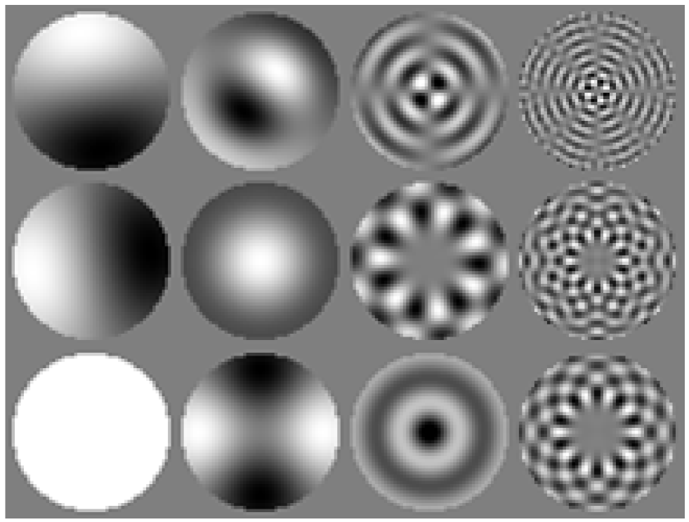
FIG. 1.: The signal-to-noise eigenmodes are plotted for a circular sky patch of $10^{\circ}$ diameter using a flat fiducial power spectrum. The modes plotted are, from left to right, top to bottom, 1, 2, 3, 4, 6, 10, 30, 50, 100, 150, 300 and 500.

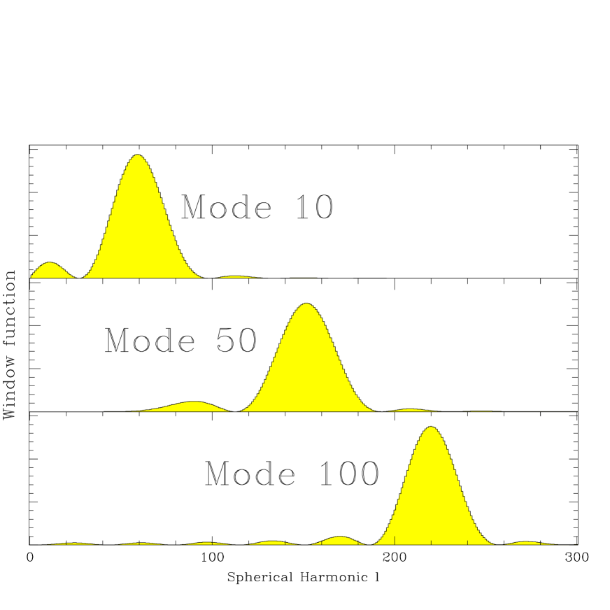
FIG. 2.: The window functions are shown for three of the signal-to-noise eigenmodes from the previous figure.

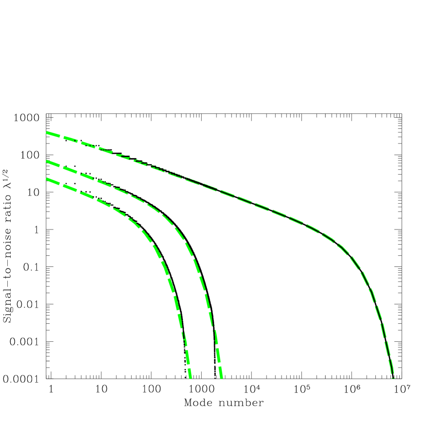
FIG. 3.: Understanding signal-to-noise eigenmodes: exact calculations and approximations. The signal-to-noise ratio $\lambda^{1/2}$ is plotted (dots) for three exact numerical calculations together with the approximation of Eq. (11) (dashed lines). From top to bottom, the three cases correspond to complete sky coverage with $w^{-1}=7\times 10^{-15}$, a disk of diameter $10^{\circ}$ with $w^{-1}=9\times 10^{-16}$, and a $5^{\circ}$ disk with $w^{-1}=2\times 10^{-15}$.

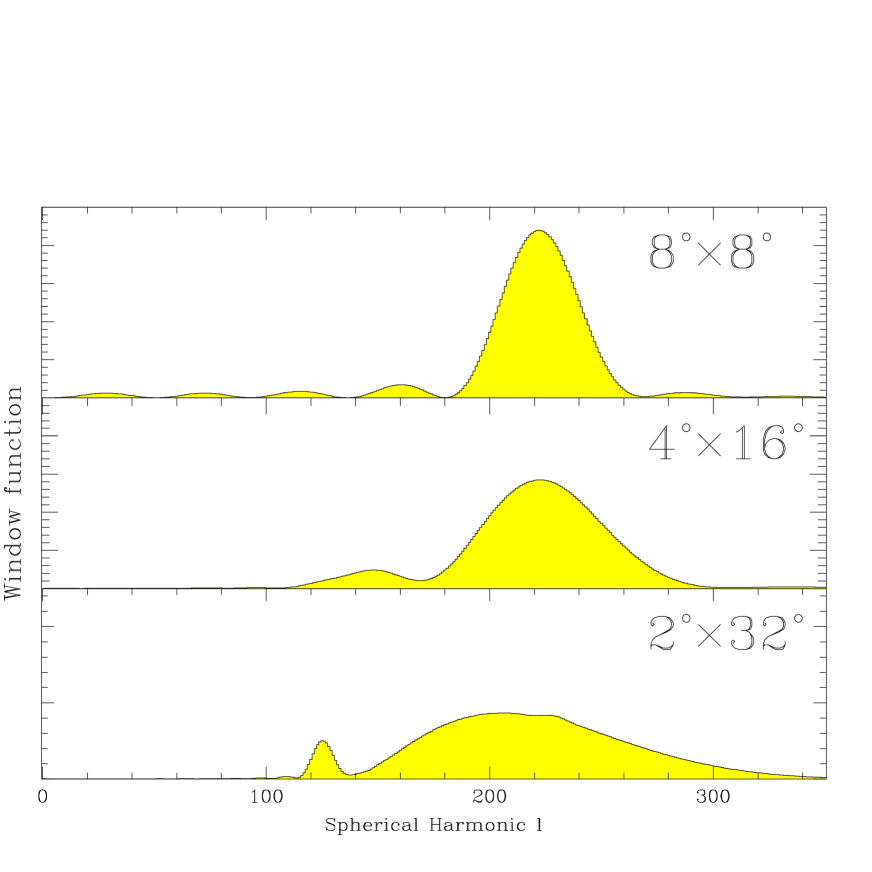
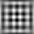
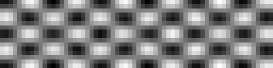
FIG. 4.: Eigenmodes in real space and Fourier space. The window functions are plotted for the signal-to-noise eigenmodes with $\l^{eff}\sim 220$ for three rectangular sky patches of the same area (64 square degrees), and are seen to be wider for the skinnier patches. The spatial eigenmodes themselves are also shown (inset).

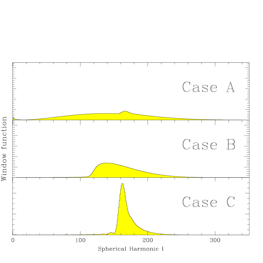
FIG. 5.: The signal-to-noise eigenmodes 53, 52 and 51 (from top to bottom) and the corresponding window functions are plotted for a $2^{\circ}\times 32^{\circ}$ rectangular sky patch.

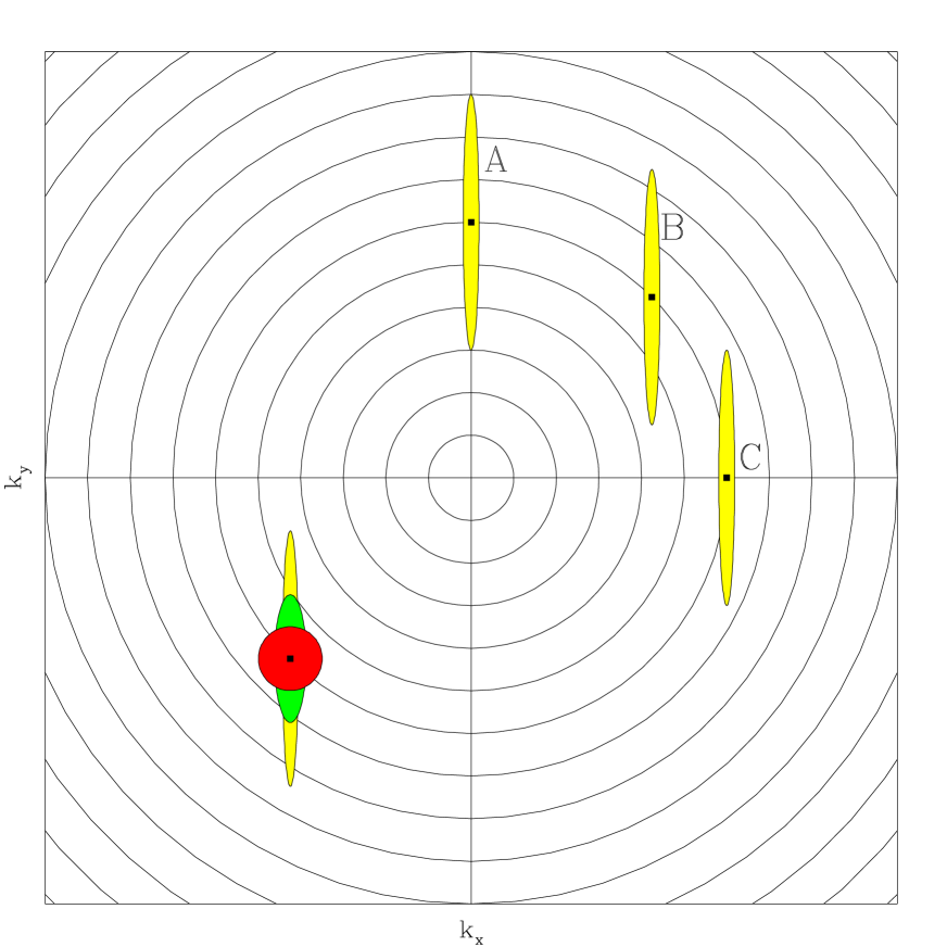
FIG. 6.: Understanding window functions. The two-dimensional Fourier transforms of the three eigenmodes from the previous figure are schematically illustrated by the ellipses at A, B and C. The width of the one-dimensional window functions corresponds to their radial extent, i.e., to how many of the circles they cross, so C gives a much narrower window than A in Fig. 5. The situation for the eigenmodes in Fig. 4 is illustrated by the ellipses to the lower left.

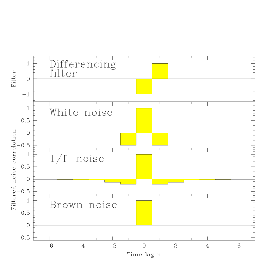
FIG. 7.: When each measurement is subtracted from the one following it (using the differencing filter in the top panel), the correlation functions resulting from white, $1/f$ and brown noise take the form shown in the three lower panels.

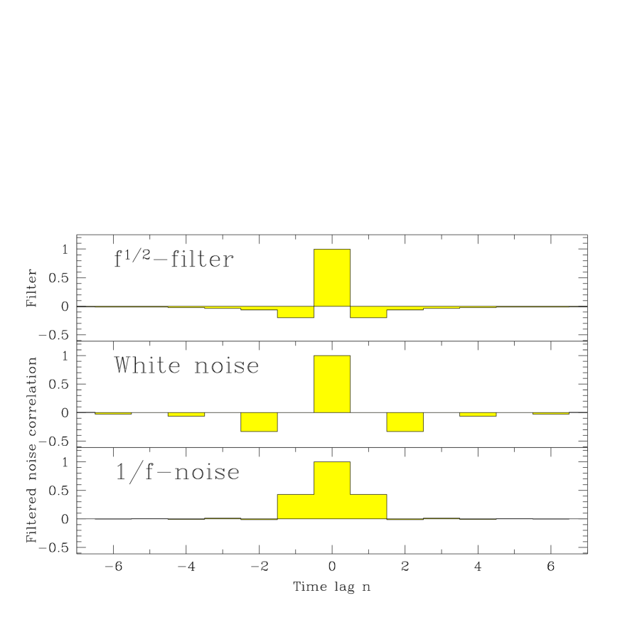
FIG. 8.: When the time stream is convolved with the “half differencing” filter in the top panel, the correlation functions resulting from white and $1/f$ noise are as shown in the lower panels. As opposed to in the previous figure, the $1/f$ correlation function does not sum to zero, which makes ${\bf M}$ band-diagonal.

FIG. 9.: Spectral functions. The top panel shows the spectral function for a sample noise covariance matrix (solid line) and its decomposition into white, 1/f and brown noise (dashed curves). The bottom panel shows the same spectral function after differencing the data (dashed curve), corresponding to multiplication with $\sin^{2}(\varphi/2)$. In the absence of brown noise (lower solid curve), $\lambda(0)=0$ which is inconvenient for computing ${\bf N}^{-1}$, but this problem can be eliminated by using different high-pass filter – the upper solid curve differs by a factor $|\sin(\varphi/2)|$.

FIG. 10.: Schematic illustration of the four scan patterns described in the text.

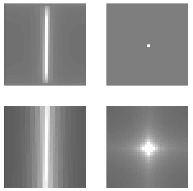
FIG. 11.: The correlation between the various pixels and the one in the center is plotted for the serpentine (upper left), grating (upper right), fence (lower left) and random (lower right) scan patterns for the case of pure $1/f$ noise.

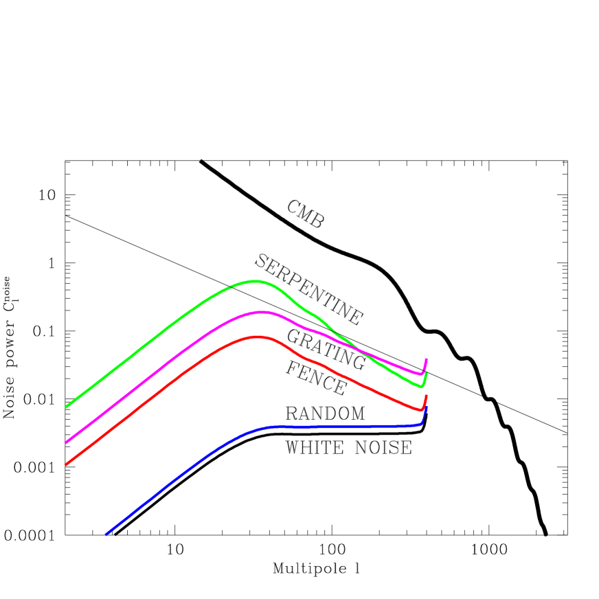
FIG. 12.: The noise power spectrum $C^{noise}_{\l}$ is plotted for our four scan patterns given pure $1/f$ noise. The corresponding noise power for white detector noise (which is identical for the serpentine, fence and random scans) is plotted below for comparison, as well as a standard CDM power spectrum (top). The straight line has slope $\l^{-1}$, just like the serpentine and fence power spectra.

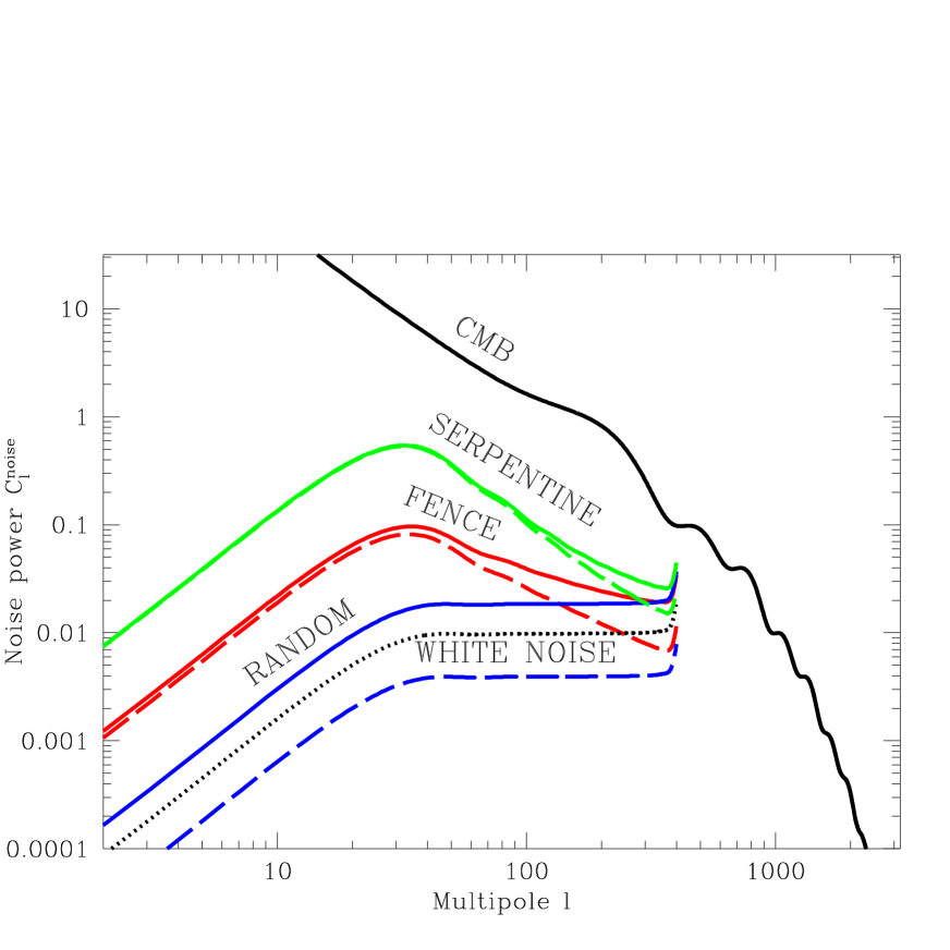
FIG. 13.: The noise power spectrum $C^{noise}_{\l}$ is plotted for the serpentine, fence and random scans with a combination of white and $1/f$ noise (solid curves), only the $1/f$ component (dashed curves) and only the white component (dotted curve, identical for all three scan patterns). A standard CDM power spectrum is plotted for comparison (top).

REFERENCES

- [1] D. Scott, M. Srednicki & M. White, ApJ 421, L5 (1994).
- [2] M. Tegmark, MNRAS 280, 299 (1996).
- [3] L. Knox, Phys. Rev. D 48, 3502 (1995).
- [4] M. Tegmark and G. Efstathiou, MNRAS 281, 1297 (1996).
- [5] G. Hinshaw, C.L. Bennett & A. Kogut, ApJ 441, 1 (1995).
- [6] G. Jungman, M. Kamionkowski, A. Kosowsky, and D. N. Spergel, Phys. Rev. Lett. 76, 1007 (1996).
- [7] M. Tegmark, A. N. Taylor, and A. F. Heavens, ApJ 480, 22 (1997).
- [8] G. Jungman, M. Kamionkowski, A. Kosowsky, and D. N. Spergel, Phys. Rev. D 54, 1332 (1996).
- [9] J. R. Bond, G. Efstathiou, and M. Tegmark, preprint astro-ph/9702100.
- [10] M. Zaldarriaga, D. Spergel, and U. Seljak 1997, preprint astro-ph/9702157.
- [11] J. R. Bond et al., Phys. Rev. Lett. 72, 13 (1994). J. R. Bond, R. L. Davis & P. J. Steinhardt, Astroph. Lett. Comm. 32, 53 (1995). J. R. Bond 1994, preprint astro-ph/9406075, in Relativistic Cosmology, proc. of 8th Nishinomiya-Yukawa Memorial Symposium (Universal Academy Press, Tokyo, 1994), p23.
- [12] J. Magueijo & M. P. Hobson, preprint astro-ph/9610105.
- [13] M. P. Hobson & J. Magueijo, MNRAS 283, 1133 (1996).
- [14] M. A. Janssen et al. 1996, preprint astro-ph/9602009.
- [15] E. L. Wright 1996, preprint astro-ph/9612006.
- [16] M. Tegmark, ApJL 480, L87 (1997).
- [17] M. Tegmark, Phys. Rev. D 55, 5895 (1997).
- [18] L. Knox, J. R. Bond, and A. H. Jaffe 1997, preprint astro-ph/9702110.
- [19] L. Lnox, ApJ 480, 72 (1997).
- [20] J. R. Bond, Phys. Rev. Lett. 74, 4369 (1995). J. R. Bond, in Cosmology and Large Scale Structure, Les Houches Section LX, edited by R. Schaeffer, J. Silk, M. Spiro, and J. Zinn-Justin 469 (Elsevier, Amsterdam, 1996), p469. J. R. Bond, in Proc. of the IUCAA dedication ceremonies, edited by T. Padmanabhan (Wiley, New York, 1994).
- [21] E. F. Bunn and N. Sugiyama, ApJ 446, 49 (1995).
- [22] E. F. Bunn, Ph.D. Thesis, U.C. Berkeley (1995), ftp pac2.berkeley.edu/pub/bunn.
- [23] K. Karhunen, Über lineare Methoden in der Wahrscheinlichkeitsrechnung (Kirjapaino oy. sana, Helsinki, 1947).
- [24] A. H. Jaffe, L. Knox, and J. R. Bond 1997, preprint astro-ph/9702109.
- [25] K. M. Górski, ApJ 430, L85 (1994).
- [26] M. Tegmark and E. F. Bunn, ApJ 455, 1 (1995).
- [27] G. Hinshaw et al., ApJL 464, L17 (1996).
- [28] W. N. Brandt et al., ApJ 424, 1 (1994).
- [29] S. Dodelson, ApJ 482, 577 (1997).
- [30] H. A. Feldman, N. Kaiser, and J. A. Peacock, ApJ 426, 23 (1994).
- [31] W. Hu, N. Sugiyama, and J. Silk, Nature 386, 37 (1997).
- [32] L. Randall, M. Soljacic, and A. H. Guth, Nucl. Phys. B 472, 377 (1997).
- [33] P. J. Davis, Circulant Matrices (Wiley, New York, 1979).
- [34] G. W. Ford, M. Kac & P. Mazur, J. Math. Phys. 6, 504 (1965).