[]

CMB polarization as a direct test of Inflation

Abstract

We study the auto-correlation function of CMB polarization anisotropies and their cross correlation with temperature fluctuations as probe of the causal structure of the universe. Because polarization is generated at the last scattering surface, models in which fluctuations are causally produced on sub-horizon scales cannot generate correlations on scales larger then $\sim 2^{o}$. Inflationary models, on the other hand, predict a peak in the correlation functions at these scales: its detection would be definitive evidence in favor of a period of inflation. This signal could be detected with the next generation of satellites.

Temperature anisotropies in the Cosmic Microwave Background (CMB) are one of the best probes of the early universe. CMB measurements are likely to answer one of the fundamental questions in cosmology: the origin of the fluctuations that formed the galaxies and the large-scale structure. If the fluctuations are consistent with current models of structure formation, then accurate measurements of the fluctuations could lead to a precise determination of a large number of cosmological parameters [1].

There are two competing sets of theories for structure formation: defect models, where a symmetry breaking phase transition generates seeds that form sub-horizon scale density fluctuations, and inflationary models, where a period of superluminal expansion turns quantum fluctuations into super-horizon density perturbations. A fundamental difference between these two mechanisms of structure formation is that only inflation alters the causal structure of the very early universe and is able to create correlations on super-horizon scales.

The COBE satellite observed correlations on angles much larger than that subtended by the horizon at decoupling $(\theta_{h}\sim 1.1^{o})$ in the CMB temperature. This does not; however, imply that there were correlations on super horizon scales at decoupling because a time dependent gravitational potential will produce temperature fluctuations at late-times, the integrated Sachs Wolfe effect (ISW). For example, cosmic string or texture models predict that most of the fluctuations observed by COBE were produced at $z<10$.

Measurements of temperature fluctuations at small scales have been suggested as a potential test of inflation: inflationary models and most non-inflationary ones predict different locations and relative heights for the acoustic peaks [2]. Unfortunately, causality alone is insufficient to distinguish inflationary and non-inflationary temperature power spectra: causal sources that mimic exactly the inflationary pattern of peaks can be constructed [3]. While the predicted CMB fluctuations of the current family of defect models differ significantly from inflationary predictions[4], it is useful to have model independent tests of the causal structure of the early universe.

Polarization fluctuations are produced by Thomson scatterings during the decoupling of matter and radiation. Thus, unlike temperature fluctuations, they are unaffected by the ISW effect. Measurements of the polarization fluctuations are certain to probe the surface of last scatter. Hence, the detection of correlated polarization fluctuations on super-horizon scales at last scattering are a definitive signature of the existence of super-horizon scale fluctuations, one of the distinctive predictions of inflation.

We will work in the initially unperturbed synchronous gauge, where the metric is given by $ds^{2}=a^{2}(\tau)[-d\tau^{2}+(\delta_{ij}+h_{ij})dx^{i}dx^{j}]$. We will consider only perturbations produced by scalar modes and will solve the Einstein equations in the presence of sources (e.g., defects) using the stiff approximation [5]. The sources are characterized by their covariantly conserved stress energy tensor $\Theta_{\mu\nu}$. Before recombination, matter and radiation act as a very tightly coupled fluid, so the evolution of fluctuations can be described by

$$\ddot{\delta}_{C}+{\frac{\dot{a}}{a}}\dot{\delta}_{C} = 4\pi G(\sum_{N}(1+3c_{N}^{2})\rho_{N}\delta_{N}+\Theta_{00}+\Theta)$$ (1)

$$\dot{\delta}_{R} = {\frac{4}{3}}\dot{\delta}_{C}-{\frac{4}{3}}\nabla\cdot{\bf{v_{R}}}$$ (2)

$$\dot{{\bf{v_{R}}}} = -(1-3c_{S}^{2}){\frac{\dot{a}}{a}}{\bf v_{R}}-{\frac{3}{4}}c_{S}^{2}\nabla\delta_{R},$$ (3)

where $\Theta/3$ is the pressure, $\delta_{R}$ and ${\bf{v_{R}}}$ describe the energy density and velocity of the photon-baryon fluid and $\delta_{C}$ is the energy density of cold dark matter. In synchronous gauge, the cold dark matter has zero velocity. The sum over $N$ is carried out over all species and $c_{S}$ is the sound speed. Temperature and polarization anisotropies seen on the sky today depend on $\delta_{R}$ and ${\bf{v_{R}}}$ at decoupling.

Equations (3) imply that the photon-baryon fluid propagates information at the speed of sound and thus cannot generate correlations on scales larger than the sound horizon. Causality on the other hand implies that the unequal time correlators of the sources $\langle\Theta_{\mu\nu}(r,\tau)\Theta_{\mu\nu}(0,\tau^{\prime})\rangle$ vanishes if $r>\tau+\tau^{\prime}$. In the absence of initial correlations, these two conditions together imply that $\langle X|_{\tau_{*}}(\hat{{\bf n}}_{1})X|_{\tau_{*}}(\hat{{\bf n}}_{2})\rangle=0$ if $\theta_{12}>2\theta_{h}\sim 2^{o}$, where $X={\delta}_{R},{\bf v_{R}},\partial_{i}{\bf v_{R}}$ and $\tau_{*}$ is the conformal time of decoupling.

In the thin scattering surface approximation, equations (3) are solved up to recombination and then the photons free stream to the observer. The final temperature anisotropy in direction $\hat{{\bf n}}$ on the sky is

$$T(\hat{{\bf n}})={\frac{\delta_{R}}{4}}|_{\tau_{*}}-\hat{{\bf n}}\cdot{\bf{v_{R}}}|_{\tau_{*}}-{\frac{1}{2}}\int_{\tau_{*}}^{\tau_{0}}d\tau\dot{h}_{ij}\hat{{\bf n}}^{i}\hat{{\bf n}}^{j}.$$ (4)

The first two terms are evaluated at the last scattering surface and the third term is an integral along the line of sight, the ISW effect. In non-inflationary models, the first two terms cannot correlate temperature fluctuations at separations larger than $2\theta_{h}\sim 2^{o}$ but because anisotropies can be created later through the ISW effect these models can have temperature correlations on larger angular scales.

Polarization is produced by Thomson scattering of radiation with a non zero quadrupole moment at the last scattering surface. The photons that scattered off a given electron came from places were the fluid had velocity ${\bf{v_{R}}}$ and thus because of the tight coupling the photon distribution function had a dipole $T_{1}=\hat{{\bf n}}\cdot{\bf{v_{R}}}$. Furthermore gradients in the velocity field across the mean free path of the photons ($\lambda_{p}$) created a quadrupole $T_{2}=\lambda_{p}n^{i}n^{j}\partial_{i}v_{Rj}$ in the photon distribution “seen” by each electron. This quadrupole generates polarization through Thomson scattering.

Linear polarization is described by a $2\times 2$ traceless tensor fully specified by the $Q$ and $U$ Stokes parameters [6]. These parameters depend on the direction of observation $\hat{{\bf n}}$ and on the orientation of the coordinate system perpendicular to $\hat{{\bf n}}$, $(\hat{{\bf e}}_{1},\hat{{\bf e}}_{2})$ used to define them. Two independent combinations with spin $\pm 2$ provide a more convenient description, $Q\pm iU$. Under rotation of the $(\hat{{\bf e}}_{1},\hat{{\bf e}}_{2})$ basis by an angle $\psi,$ this combinations transform as $(Q^{\prime}\pm iU^{\prime})=\exp({\mp 2i\psi})\ (Q\pm iU)$, and can be expanded in spin $\pm 2$ harmonics, $(Q\pm iU)(\hat{{\bf n}})=\sum_{lm}a_{\pm 2,lm}\ \ {}_{\pm 2}Y_{l}^{m}(\hat{{\bf n}})$ [7]. An equivalent expansion using tensors on a sphere can be found in [8]. The scattered radiation field is given by $(Q+iU)=-3/4\sigma_{T}\int d\Omega^{\prime}/4\pi({\bf m}\cdot\hat{{\bf n}}^{\prime})T_{2}(\hat{{\bf n}}^{\prime})\propto\lambda_{p}{\bf m}^{i}{\bf m}^{j}\partial_{i}v_{j}|_{\tau_{*}}$, where $\sigma_{T}$ is the Thomson scattering cross section and we have written the scattering matrix as $P({\bf m},\hat{{\bf n}}^{\prime})=-3/4\sigma_{T}({\bf m}\cdot\hat{{\bf n}}^{\prime})^{2}$ with ${\bf m}=\hat{{\bf e}}_{1}+i\hat{{\bf e}}_{2}$ . In the last step, we integrate over all directions of the incident photons $\hat{{\bf n}}^{\prime}$.

As photons decouple from the baryons their mean free path is growing very rapidly, so a more careful analysis is needed to get the final polarization [9],

$$(Q+iU)(\hat{{\bf n}})\approx 0.17\Delta\tau_{*}{\bf m}^{i}{\bf m}^{j}\partial_{i}v_{j}|_{\tau_{*}}$$ (5)

where $\Delta\tau_{*}$ is the width of the last scattering surface and is giving a measure of the distance photons can travel between their last two scatterings. The appearance of ${\bf m}$ in equation (5) assures that $(Q+iU)$ transforms correctly under rotations of $(\hat{{\bf e}}_{1},\hat{{\bf e}}_{2})$. Equation (5) shows that the observed polarization only depends on the state of the fluid at the last scattering surface. No correlations can be present in the polarization for separations larger than $\sim 2^{o}$ in non-inflationary models.

Polarization can be decomposed into two distinct parts[7]: $E$ and $B$ with $a_{E,lm}=-(a_{2,lm}+a_{2,lm})/2$ and $a_{B,lm}=-(a_{2,lm}-a_{2,lm})/2i$ . Only four power spectra are needed to describe the full radiation field, three autocorrelations $C_{Xl}={\frac{1}{2l+1}}\sum_{m}\langle a_{X,lm}^{*}a_{X,lm}\rangle$ for $X=T,E,B$ and the cross correlation between $E$ and $T$, $C_{Cl}={\frac{1}{2l+1}}\sum_{m}\langle a_{T,lm}^{*}a_{E,lm}\rangle$.

Density perturbations only contribute to $E$ [7, 8]. We can illustrate this point using equation (5) and for convenience choosing $\hat{{\bf n}}=\hat{{\bf z}}$ and ${\bf m}=\hat{{\bf x}}+i\hat{{\bf y}}$. In the small scale limit, we have $\nabla^{2}B=(\partial_{y}^{2}-\partial_{x}^{2})U+2\partial_{x}\partial_{y}Q$ [7] (where $\nabla^{2}=(\partial_{y}^{2}+\partial_{x}^{2})$ is the 2-d Laplacian). This gives $\nabla^{2}B=-\nabla^{2}(\hat{{\bf z}}\cdot{\bf{\nabla}\times{v_{R}})}$ and is zero because the velocity field produced by density perturbations is irrotational.

The correlation functions of $Q$ and $U$ can be defined in a way which makes them independent of the coordinate system [8], given two directions in the sky we first rotate $(\hat{{\bf e}}_{1},\hat{{\bf e}}_{2})$ in each direction so that both $\hat{{\bf e}}_{1}$ are aligned with the great circle connecting the two points. We then use the $Q$ and $U$ as measured in this system to compute the correlation functions which depend only on $\theta$ the angle between the two directions. They are given by,

$$C^{(Q,U)}(\theta) = \sum_{l}{\frac{2l+1}{4\pi}}[C^{(E,B)}_{l}\ F^{1}_{l}(\theta)-C^{(B,E)}_{l}\ F^{2}_{l}(\theta)]$$ (6)

where $\ {}_{\pm 2}Y_{l}^{2}(\theta,\phi)=\sqrt{(2l+1)/4\pi}\ [F^{1}_{l}(\theta)\pm F^{2}_{l}(\theta)]\ \exp{(2i\phi)}$. Both correlation functions receive contributions from the $E$ and $B$ channels. The $E$ channel contains all the cosmological signal if there are no tensor or vector modes.

We computed both $C^{(Q,U)}(\theta)$ for the model proposed by Turok which has a clever choice of source stress energy tensor that is able to reproduce the pattern of peaks of inflationary standard CDM (sCDM)[3]. The results are shown in figure 1. We see that the inflationary model is able to produce correlations on angular scales larger than $\sim 2^{o}$, while the other model cannot. On smaller angular scale than shown in figure 1, the two correlation functions coincide. The difference between the two models is a result of the causal constraints and is insensitive to source evolution. It is also worth pointing out that in inflationary models the large scale polarization is suppressed relative to the small scale signal, so we are after a small effect.

Next, we estimate the expected uncertainties in measuring $C^{(Q,U)}(\theta)$. Since receiver noise is the likely to be the dominant source of variance, we can make a simple estimate of the total noise: it is proportional to the number of independent pairs of pixels, $N_{p},$ at a given separation, $\theta$. For an experiment with a full width at half maximum of $\theta_{fwhm},$ $N_{p}=1/2\times(4\pi/\theta_{fwhm}^{2})\times(2\pi\theta/\theta_{fwhm})$. If $\sigma_{(Q,U)}^{2}$ is the noise in the polarization measurement per resolution element, then the noise in the cross correlation is given by $\Delta C^{(Q,U)}=\sqrt{2/N_{p}}\ \sigma_{(Q,U)}^{2}\approx 20\ w_{P}^{-1}\sqrt{0.2^{o}/\theta_{fwhm}}\sqrt{2^{o}/\theta}$ where $w_{P}^{-1}=\sigma_{(Q,U)}^{2}\ \Omega_{pix}/4\pi$.

We can make a more accurate determination of the noise using the covariance matrix of the different power spectra[7]:

$${\rm Cov}(\hat{C}_{(E,B)l}^{2}) = {2\over 2l+1}(\hat{C}_{(E,B)l}+w_{P}^{-1}e^{l^{2}\sigma_{b}^{2}})^{2}$$ (7)

which give the following variances for the correlation functions,

$$(\Delta C^{(Q,U)})^{2} = \sum_{l}({2l+1\over 4\pi})^{2}\{{\rm Cov}(C^{2}_{(E,B)l})\ [F^{1}_{l}(\theta)]^{2}$$ (9)

$$+{\rm Cov}(C^{2}_{(B,E)l})\ [F^{2}_{l}(\theta)]^{2}\}.$$

Figure 1 shows the noise in each correlation, in the limit where the variances are dominated by receiver noise $(\Delta C^{Q})^{2}=(\Delta C^{U})^{2}$ and agree perfectly with our previous estimates. If either the cosmic variance is important or the power spectra of $E$ and $B$ differ, then the approximate estimate of the previous paragraph is not accurate and the full calculation should be used to estimate the noise.

The noise in the correlation functions can be reduced by focusing on the $E$-like piece of the polarization. The noise in the both $C^{(Q,U)}(\theta)$ receives contributions from the variances in both the $E$ and $B$ spectra, but by computing both contributions separately we can show that the variance in $E(B)$ makes the dominant contribution to $\Delta C^{Q}(\Delta C^{U})$. If we filter the maps to pull out only the $E$ component, then we remove not only the $B$ signal but also some of the noise, $\Delta C^{U}$ goes down almost by a factor of $\sim 4$. The assumption that most of the signal is in the $E$ channel can be checked within the data as both $E$ and $B$ contributions can be measured separately from the maps.

For the MAP satellite, without filtering the noise, $\Delta C^{(Q,U)}\approx 0.36/\sqrt{\theta}\ \mu K^{2}$, so it will not be sensitive enough to detect this signal, even if we combine all of the three highest frequencies. However, if we filter the map to extract the E channel signal, then the noise in the MAP experiment drops to $\Delta C^{U}\sim 0.1/\sqrt{\theta}\ \mu K^{2}$, and the $C^{U}$ signal should be detectable. The PLANCK satellite, with its very sensitive bolometers, should be able to achieve $\Delta C^{(Q,U)}\approx 0.003/\sqrt{\theta}\ \mu K^{2}$ and should easily be able to detect both $C^{U}$ and $C^{Q}$. As cosmic variance is not the dominant contribution to the noise, an experiment observing a small patch of the sky could also potentially detect this signal.

The temperature-polarization cross-correlation [10] is another potential test of the origin of fluctuations: although ISW effects produce temperature fluctuations after decoupling, we still do not expect correlations between temperature and polarization on large angular scales for defect models. The correlations between temperature and polarization fluctuations directions $\hat{\bf n}_{1}$ and $\hat{\bf n}_{2}$ are,

$$\langle Q(\hat{\bf n}_{1})T(\hat{\bf n}_{2})\rangle=\langle Q_{1}^{*}T_{2}^{*}\rangle-{1\over 2}\int_{\tau_{*}}^{\tau_{0}}d\tau\hat{\bf n}_{1}^{i}\hat{\bf n}_{1}^{j}\langle\dot{h}_{ij}(\tau)Q^{*}_{1}\rangle,$$ (10)

$T^{*}$ stands for the first two terms in equation (4) and $Q^{*}$ is given by equation (5).

In the polarization temperature cross correlation, only the term involving the line of sight integration could produce correlations on large angular scales. This would require correlations between the late time variations of the metric and the velocity at last scattering. For this to occur in defect models, they must be moving very fast and remain coherent as they evolve from recombination to very late times. As figure 1(c) shows, even Turok’s causal seed model, which mimics inflation remarkable well in the temperature correlation does not predict any temperature-polarization correlation.

If gravity waves, rather than scalar modes, were the dominant source of the anisotropies, then they could, in principle, create large angular scales cross correlations. However, if gravity waves were significant enough to create a large signal, then they would be directly detectable in the B channel.

Figure 1(c) shows the calculated values of the cross correlation together with the expected noise. The signal is well above the noise for MAP and Planck. The detection of a large angular scale cross correlation with no appreciable signal in the polarization $B$ channel would put very stringent limits on the physics of models trying to mimic inflation.

There is only one caveat to our argument: reionization. If the universe reionized very early, a significant fraction of the observed polarization will come from the rescattering of photons at late times. In most scenarios, the fraction of rescattered photons is thought to be less than $\sim 20\%$ [11]. Reionization has two effects on our argument. First, it reduces the amplitude of the correlation function by a factor $\exp{(-2\tau)}$, where $\tau$ is the optical depth to decoupling ($\tau\leq 0.2$). Second, it creates further structure in the correlation function on large angular scales. Fortunately, the effect of reionization can be separated from that of the primordial anisotropies: it leaves a very specific signature in the power spectrum, a peak at very low $l$ that is easily distinguish from the $l^{6}$ dependence expected from causality constrains alone [12, 13, 14]. Because of the form of $F_{l}^{1}(\theta)$ and $F_{l}^{2}(\theta)$, this peak produces an almost constant positive offset in $C^{Q}$ and $C^{U}$ for angles $\theta\sim 2^{o}$. Because the offset in $C^{U}$ is positive $(F^{2}_{l}(\theta)<0$ for $\theta\sim 2^{o}$ and $l<70$) reionization at a relatively recent epoch can never create the negative peak at $\theta\sim 2^{o}$ predicted by inflationary models.

There is a precise signature in $C^{(Q,U)}(\theta)$ on $\sim 2^{o}$ scales that would allow an unambiguous test of inflation. The signal is small, but within reach for the new generation of experiments. The cross correlation between temperature and polarization is also expected to provide strong constraints that could distinguish inflation from non-inflationary models: this signal is much larger and will be well above the noise for MAP. The next generation of satellites or even polarization measurements from the ground could provide a definitive test of the inflationary paradigm in the relatively near future.

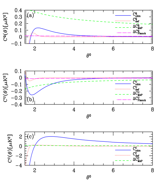
FIG. 1.: Correlation functions for Q (a) and U (b) Stokes parameters for sCDM and the causal seed model discussed in the text. The noise in their determination is shown for both MAP and Planck. Panel (b) shows the expected noise for MAP if the CMB maps are flltered to include only the $E$ channel signal. Panel (c) shows the cross correlation between temperature and polarization and the noise for MAP, the expected variance for Planck is even smaller. Each resolution element in the correlation function should be considered independent.

- [1] D.N. Spergel, 1994 Warner Prize Lecture, Bull. Amer. Astron. Soc., 26, 1427 (1994); G. Jungman et al. M. Kamionkowski, A. Kosowsky, and D. N. Spergel, Phys. Rev. Lett. 76, 1007 (1996); ibid Phys. Rev. D 54 1332 (1996); J.R. Bond, G. Efstathiou & M. Tegmark, Report no. astro-ph/9702100; M. Zaldarriaga, D. N. Spergel and U. Seljak, Report no. astro-ph/9702157, 1997 (unpublished).
- [2] W. Hu and M. White, Astrophys. J. 471 30 (1996); W. Hu, D. Spergel and M. White, Phys. Rev D 55, 3288 (1997).
- [3] N. Turok, Phys. Rev. Lett. 77, 4138 (1996); ibid Phys. Rev. D 54 3686 (1996).
- [4] U. Pen, U. Seljak and N. Turok, Report no.astro-ph/9704165, 1997 (unpublished).
- [5] S. Veeraraghavan and A. Stebbins, Astrophys. J. 365 37 (1990).
- [6] Circular polarization cannot be generated in the early universe through the process of Thomson scattering, so Stokes parameter is 0.
- [7] M. Zaldarriaga and U. Seljak, Phys. Rev. D 55 1830 (1997); U. Seljak and M. Zaldarriaga Phys. Rev. Lett. 78, 2054 (1997).
- [8] M. Kamionkowski et al., Report no. astro-ph/9609132, ibid astro-ph/9611125, 1996 (unpublished).
- [9] M. Zaldarriaga and D. Harari, Phys. Rev. D 52 3276 (1995).
- [10] D. Coulson, R. Crittenden and N. Turok, Phys. Rev. Lett. 73. 2390 (1994)
- [11] Z. Haiman, and A. Loeb, astro-ph/9611028, 1996 (unpublished).
- [12] M. Zaldarriaga, Phys. Rev. D 55 1822 (1997).
- [13] W. Hu and M. White, astro-ph/9702170, 1997 (unpublished).
- [14] R. Battye, private communication.