ON THE COMPUTATION OF CMBR ANISOTROPIES FROM SIMULATIONS OF TOPOLOGICAL DEFECTS

Abstract

Techniques for computing the CMBR anisotropy from simulations of topological defects are discussed with an eye to getting as much information from a simulation as possible. Here we consider the practical details of which sums and multiplications to do and how many terms there are.

Probably the most fruitful field of cosmological observation in the past few years comes from observations of the anisotropies of the Cosmic Microwave Background Radiation (CMBR). One of the first and the most dramatic detections was made by the DMR on the COBE satellite over 5 years ago. New results continue to pour in and we can expect this continue to at least until the Planck experiment provides us with an exquisitely detailed all-sky map in about a decade. Theoretical modeling of the data and their interpretation in terms of cosmogenic theories has generally been able to keep pace with these observations but we can expect the observational data to become increasingly more precise. There are models such as inflation where the statistical properties of the anisotropy pattern is well described as being statistically isotropic Gaussian random noise where the parameters describing the Gaussian distribution can be computed by solving linear sets of ordinary differential equations. For such models a complete statistical description is fairly easy to obtain and the predictions are routinely made made with better than 1% accuracy. In another class of theories, where the inhomogeneities are seeded by topological defects, it is not clear whether we will ever obtain this kind of accuracy. Of course this may be a moot point if the predictions for these models, such as they are, do not fit observations. In the paper we will discuss some of the issues involved with computing CMBR anisotropies for defect models.

One of the fundamental differences between Gaussian models and defect models is that the dynamics of the former are described by linear equations while that the latter by nonlinear equations. Linearity combined with the assumed statistical homogeneity of the universe guarantee that one may decompose the cosmological perturbations into eigenmodes, which are eigenfunctions of the generators of the isometries of the space-time, and that each eigenfunction will evolve independently. So, for example in a flat Friedmann-Robertson-Walker (FRW) spacetime, the eigenmodes could be Fourier modes which are eigenfunctions of the generator of translation. While one might have to solve the linear equations for a Fourier mode numerically, one need only solve the equation once for each value of $|{\bf k}|$. For a given type of inhomogeneity, e.g. adiabatic or isocurvature, the only freedom in the initial condition of a given mode is the amplitude, and, since the equations are linear, solutions scale linearly with the initial amplitude.

For topological defects the equations are non-linear so different eigenmodes are coupled and one does not know the evolution of one mode without taking into account the evolution of all the other. It is usually simpler to think about topological defects in real space rather than the space of eigenmodes ($k$-space). One reason is that equations describing the evolution of the defects are spatially local while they are highly non-local in $k$-space. Another reason is that causality guarantees that the range interaction does not extend beyond a certain distance, the causal horizon, while the range of interaction in $k$-space is unbounded. Causality allows one to consider a finite patch of the universe and ignore what goes on outside of that patch, at least for points more than a horizon distance away from the boundary of the patch.

In order to determine the likelihood that the observed inhomogeneities in the universe could be explained by topological defects one would need a description of the statistical ensemble of possible topological defects configurations and their evolution. In general we cannot even find analytic solution to describe the evolution of specific configurations so the way one tries to determine the statistical properties is through numerical experiment. Namely one generates a realization of the defect configuration at some early time and evolves it and the matter surrounding it according to their equations of motion. One might then try another configuration, and so on, until one has a fair statistical sample. It is generally believed that the statistical properties of the defects are ergodic so that one may also obtain a fair sample by considering a large enough volume of a single realization. One need only consider the observations predicted for observers situated in different locations in the simulation volume. Since one needs to build up a fair sample it is important to obtain as many realizations of the anisotropy as possible.

1 Geometry of Computation

Figure 1: Here is shown the geometry for large angle anisotropy computations. In the inset the cube represents the simulation volume while the sphere gives the observer’s horizon, the volume which contributes to the anisotropy pattern of a given observer. The shaded on the graph gives the range of temporal and length scales resolved by the simulation. Generally the most important missing scales are on the left, i.e. from early times. Some numbers appropriate for studying COBE scale anisotropies are given.

Numerous authors have used simulations of defects to produce realizations of anisotropy patterns from defects [1, 2, 5, 6, 7, 8, 9, 10, 11]. Some of these have been used to examine large angle anisotropies [2, 5, 6, 8, 9, 11] while others have been used to examine anisotropies on smaller angular scales [1, 7, 10]. The geometry used for these large angle numerical experiments is shown in fig 1. One must evolve the defects in a very large simulation volume, as big as the present horizon and ideally one would like to evolve from time of recombination. Usually one takes periodic boundary conditions for the defect configuration. However this periodicity does not really matter - since for most methods of laying down the defects one can show that the defect configuration in any given horizon volume is drawn from the same distribution as if one were to have simulated and infinite volume. The cubical box with periodic boundary condition are only easily implemented in the case of spatially flat FRW cosmology. Doing this computation for an open universe, as was done in by Pen and Spergel[8], is actually a more difficult problem in many respects. For simplicity we will assume a flat FRW cosmology, which allows us to make use of the Fourier series representations of distributions in the simulation box, i.e.

$$F({\bf x})=\sum_{\bf k}\widetilde{F}({\bf k})\,e^{i{\bf k}{\hskip-0.7pt\cdot\hskip-0.7pt}{\bf x}}\ .$$ (1)

We will specifically be considering a a cubical simulation volume with $N\times N\times N$ spatial resolution elements.

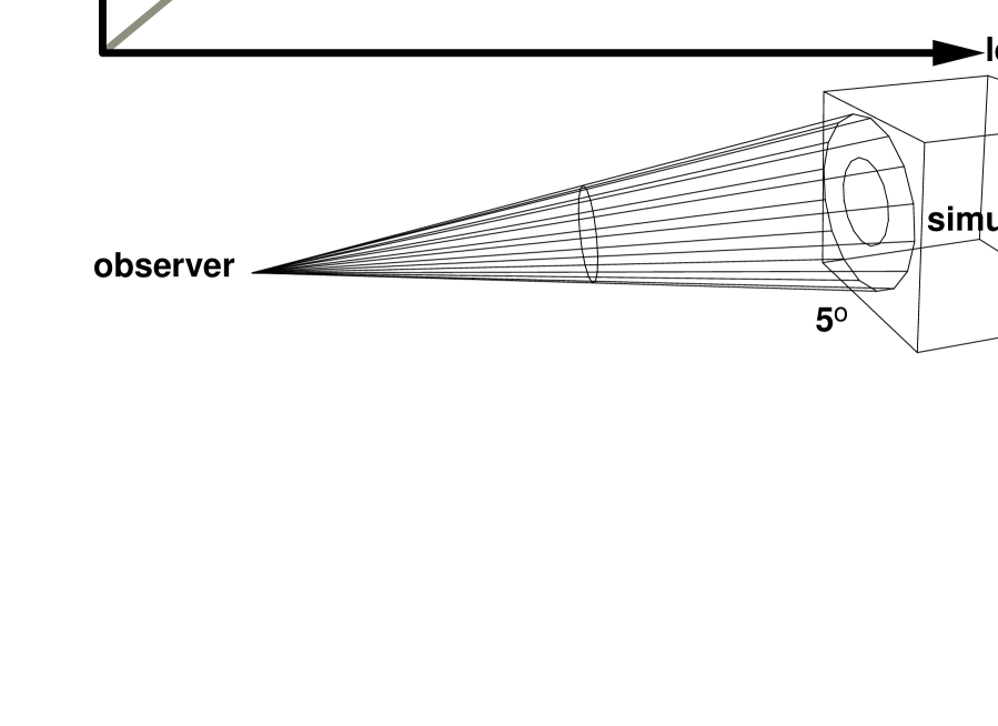
Figure 2: Here is shown the geometry for a small-angle anisotropy computations. The cube represents the simulation volume and the cone the photons from the simulation converging toward the observer. The shaded region on the graph gives the scales resolved by the simulation. The most important missing scales are on the right and left, i.e. early times and late times. Some numbers appropriate for studying degree scale anisotropy are given.

2 Dynamic Range

Given these general considerations let us proceed to consider specific issues associated with the computation of MBR anisotropies from seeds in a box of a fixed comoving size, $L$. All numerical simulations have a finite dynamical range in both spatial and temporal scales. There will be a finite spatial resolution on small scales and the size of the box itself will limit the largest accessible scale. Similarly there will be finite temporal resolution, usually related to spatial resolution by the Courant condition $\Delta t\mathrel{\mathchoice{\lower 3.6pt\vbox{\halign{$\mathsurround=0pt\displaystyle\hfil#\hfil$\cr<\crcr\sim\crcr}}}{\lower 3.6pt\vbox{\halign{$\mathsurround=0pt\textstyle\hfil#\hfil$\cr<\crcr\sim\crcr}}}{\lower 3.6pt\vbox{\halign{$\mathsurround=0pt\scriptstyle\hfil#\hfil$\cr<\crcr\sim\crcr}}}{\lower 3.6pt\vbox{\halign{$\mathsurround=0pt\scriptscriptstyle\hfil#\hfil$\cr<\crcr\sim\crcr}}}}\Delta x/c$. Here $c$ is the speed-of-light which characterizes the dynamics of most defects. For this reason the coherence length of the defects will scale with the causal horizon, so that in order to properly represent the defect configuration the finite spatial resolution leads to a minimum starting time: $t_{\rm i}\gg\Delta x$. This large characteristic velocity of the defects also means that the defect configuration will start to “see” the finite size of the box when the causal horizon reaches the box size. It is desirable to end the simulations before this happens, i.e. $t_{\rm f}\mathrel{\mathchoice{\lower 3.6pt\vbox{\halign{$\mathsurround=0pt\displaystyle\hfil#\hfil$\cr<\crcr\sim\crcr}}}{\lower 3.6pt\vbox{\halign{$\mathsurround=0pt\textstyle\hfil#\hfil$\cr<\crcr\sim\crcr}}}{\lower 3.6pt\vbox{\halign{$\mathsurround=0pt\scriptstyle\hfil#\hfil$\cr<\crcr\sim\crcr}}}{\lower 3.6pt\vbox{\halign{$\mathsurround=0pt\scriptscriptstyle\hfil#\hfil$\cr<\crcr\sim\crcr}}}}L/c$. These considerations indicate that the number of temporal resolution elements is $\sim N$.

From a box at least as large as twice the horizon one can study the very largest angle anisotropies since, as illustrated in fig 1, one does not see the periodicity of the universe. The edge of ones horizon in one direction nearly touches the edge in the opposite direction, but one is seeing this far only at the earliest times when the (causal) correlation length is arbitrarily small, so there need be no effect of periodicity at all. The finite spatial resolution in such a simulation will limit the angular resolution. If most of the anisotropy is generated at large redshifts then the angular resolution is $\Delta\theta\sim\Delta x/(L/2)\sim 2/N$, which corresponds to a largest available angular wavenumber ${l_{\rm max}}\sim N/2$.

For simulations used to compute smaller angle anisotropy, as illustrated in fig 2, the effects of periodicity are much more severe as one can “see” beyond the simulation volume. One is not really simulating a large universe as we live in, but rather a truly small and periodic one. In such a universe one would see the pattern of anisotropy to be roughly periodic on the sky. What one is hoping is that the statistical properties of each of these patches are similar to those of a similar sized patch in a non-periodic universe. The angle subtended by the simulation box gives you an upper limit on the angular scale you are probing, while the spatial resolution gives a lower limit. Clearly the range of scales probed is roughly the same as for the large-angle case: ${l_{\rm max}}/{l_{\rm min}}\sim N$. Note however that one is not assured that one has the complete picture for these scales since one also is limited in temporal scales as well (see fig 2). One could, in principle, piece together all scales by combining simulations with different box sizes and different temporal ranges. Being able to do so presupposes that the different angular and temporal scales are essentially uncorrelated. This is liable to be less true in non-Gaussian models. For example in string models, even long strings at late times which subtend a very large angle, do also exhibit temperature discontinuities which will have an effect on all angular scales. However the discontinuities from these longer strings are rare and do not contribute greatly to the smaller scale anisotropies when compared to the much more numerous smaller angle strings. The assumption of independence of scales is a good approximation but not exactly correct. Note also that the finite box size not only limits the access to large spatial scales but also to large temporal scales. Once the horizon sufficiently exceeds the box size, the seeds will behave differently than they would in an infinite universe. Thus we must also presuppose that there are no long term temporal correlations which will be different in periodized box than in an infinite box. Generally we find that seeds only produce significant perturbations on scales comparable to the horizon size and thus any long term temporal correlations which might exist cannot not have much effect on the anisotropies.

3 The Brightness Distribution

Here we would first like to point out just how much information is required to describe the photon distribution present in a simulation. Recall that in a Gaussian models the statistical distribution of the anisotropies observed by any given observer is determined completely by the ensemble-averaged angular power spectrum, i.e. the $C_{l}$’s. For angular resolution characterized by ${l_{\rm max}}$ one only needs ${l_{\rm max}}$ real numbers. Note that the $C_{l}$’s do not give the spatial correlations in the anisotropy pattern but, as this is not observable in practice, these spatial correlations are not of interest. For a non-Gaussian model where one relies on numerical experiment one really wants to use the distribution function of anisotropy patterns for all observers in the simulation. If one has $N^{3}$ spatial resolution elements and $({l_{\rm max}}+1)^{2}$ angular resolution elements then one needs naively $N^{3}({l_{\rm max}}+1)^{2}$ real numbers to describe the brightness pattern. So, for example, we could describe the brightness pattern as

$${\Delta T\over T}({\hat{\bf n}},{\bf x})=\sum_{l=0}^{l_{\rm max}}\sum_{m=-l}^{l}{a_{\scriptscriptstyle(l,m)}}({\bf x})\,{Y_{\scriptscriptstyle(l,m)}}({\hat{\bf n}};{\hat{\bf z}})\ .$$ (2)

where the ${a_{\scriptscriptstyle(l,m)}}$’s are the $N^{3}({l_{\rm max}}+1)^{2}$ real numbers (recall that $a_{\scriptscriptstyle(l,-m)}=(-1)^{m}{a_{\scriptscriptstyle(l,m)}}^{*}$ and there are thus $2l+1$ real numbers for each $l$). Since typically ${l_{\rm max}}\sim N$ this is $N^{5}$ numbers - which is a rather formidable amount of data. Note that there is some information about the uninteresting spatial correlations in these numbers. In fact one can use the spatial correlations to significantly reduce the amount of information needed to describe the brightness distribution.

The Fourier transform of eq (2) is

$${\Delta T\over T}({\hat{\bf n}},{\bf x})=\sum_{\bf k}\sum_{l=0}^{l_{\rm max}}\sum_{m=-l}^{l}{\widetilde{a}_{\scriptscriptstyle(l,m)}}({\bf k})\,{Y_{\scriptscriptstyle(l,m)}}({\hat{\bf n}};{\hat{\bf z}})\,e^{i{\bf k}{\hskip-0.7pt\cdot\hskip-0.7pt}{\bf x}}\ .$$ (3)

which still contains $N^{3}({l_{\rm max}}+1)^{2}$ real numbers. Here ${\hat{\bf n}}$ gives the direction in which the brightness is measured. The 2nd argument of ${Y_{\scriptscriptstyle(l,m)}}$, ${\hat{\bf z}}$, indicates the North pole of the spherical polar coordinates used in the spherical harmonic decomposition. In this case the $m$ decomposition has no particular physical significance. If however we rotate the spherical polar coordinates, differently for each ${\bf k}$, such that the North pole is the direction of ${\bf k}$, we obtain a more interesting decomposition:

$${\Delta T\over T}({\hat{\bf n}},{\bf x})=\sum_{\bf k}\sum_{l=0}^{l_{\rm max}}\sum_{m=-l}^{l}{\Delta_{\scriptscriptstyle(l,m)}}({\bf k})\,{Y_{\scriptscriptstyle(l,m)}}({\hat{\bf n}};{\hat{\bf k}})\,e^{i{\bf k}{\hskip-0.7pt\cdot\hskip-0.7pt}{\bf x}}.$$ (4)

Mathematically this rotation is given by

$${\widetilde{a}_{\scriptscriptstyle(l,m)}}({\bf k})=\sum_{m^{\prime}=-l}^{l}D^{l}_{m,m^{\prime}}({\hat{\bf z}},{\hat{\bf k}})\,{\Delta_{\scriptscriptstyle(l,m)}}({\bf k})\ ,$$ (5)

where the $D^{l}_{m,m^{\prime}}$ are Wigner rotation matrices defined by

$$D^{l}_{m,m^{\prime}}({\hat{\bf z}},{\hat{\bf k}})=\int d^{2}{\hat{\bf n}}\,Y^{*}_{\scriptscriptstyle(l,m)}({\hat{\bf n}};{\hat{\bf z}})\,Y_{\scriptscriptstyle(l,m^{\prime})}({\hat{\bf n}};{\hat{\bf k}})$$ (6)

which obey the sum rule

$$\sum_{m=-l}^{l}D^{l}_{mm_{1}}({\hat{\bf z}},{\hat{\bf k}})\,D^{l*}_{mm_{2}}({\hat{\bf z}},{\hat{\bf k}})=\delta_{m_{1}m_{2}}.$$ (7)

The $m$ decomposition of eq (4) is useful is because the different $m$’s correspond to the different helicities of the brightness pattern. In linear theory (i.e. small perturbations) the different helicities of the brightness pattern only couple to different components of the gravitational field. In particular $m=0$ couples to scalar perturbations, $m=\pm 1$ to vector perturbations, and $m=\pm 2$ to tensor perturbations. Helicities with $|m|>2$ are not coupled to the gravitational field at all. Any brightness anisotropy with $|m|>2$ helicities, with no gravitational “forcing terms”, would be damped to zero by scattering of the photons. Thus we expect that the brightness pattern in our universe to only have helicities with $|m|\leq 2$, i.e. scalar, vector, and tensor modes. It would indeed be interesting, as a check of this notion, to decompose the brightness pattern in our patch of the universe into helicities. However this requires a knowledge of the spatial pattern of anisotropies, and we cannot expect to measure this anytime soon. Nevertheless, in a simulation we do know the spatial pattern, and we may use the helicity decomposition, as a form of data compression by ignoring the ${\Delta_{\scriptscriptstyle(l,m)}}$’s with $|m|>2$ which we know a priori to be zero. By doing so we have reduced the amount of data required to describe the brightness pattern to $5{l_{\rm max}}N^{3}\sim N^{4}$, i.e. reducing the dimensionality by one. The special “helicity state” of the CMBR brightness pattern has long been understood[12] and is implicit in most anisotropy computations, but the transformation between helicities and the spatial brightness distribution is rarely used as it is not needed in Gaussian theories.

In Gaussian theories the brightness pattern is described by the $C_{l}$’s and in non-Gaussian theories the $C_{l}$’s still exist but do not give the entire picture. Since the $C_{l}$’s give the expectation value of the $|{a_{\scriptscriptstyle(l,m)}}|^{2}$ averaged over all realizations one cannot determine their values from a single simulation. However, just as we do on Earth, each one can construct an unbiased estimator of the $C_{l}$ for each observer position in the simulation

$$\widehat{C}_{l}({\bf x})=\sum_{m=-l}^{l}{|{a_{\scriptscriptstyle(l,m)}}({\bf x})|^{2}\over 2l+1}.$$ (8)

and, assuming ergodicity, one should take a volume average of the estimators from all the observers:

$$\overline{\widehat{C}_{l}}={1\over V}\int d^{3}{\bf x}\,\widehat{C}_{l}({\bf x})=\sum_{\bf k}\sum_{m=-l}^{l}{|{\Delta_{\scriptscriptstyle(l,m)}}({\bf k})|^{2}\over 2l+1}\ .$$ (9)

This is the best estimator one can obtain from a single simulation. To obtain the 2nd equality in this equation the orthonormality of the $e^{i{\bf k}{\hskip-0.7pt\cdot\hskip-0.7pt}{\bf x}}$ and the sum rule for $D^{l}_{mm^{\prime}}$’s has been used. Since only scalar, vector, and tensor modes contribute one may rewrite this as

$$\overline{\widehat{C}_{l}}=\overline{\widehat{C}_{l}^{\rm S}}+\overline{\widehat{C}_{l}^{\rm V}}+\overline{\widehat{C}_{l}^{\rm T}}$$ (10)

where

$$\overline{\widehat{C}_{l}^{\rm S}} = \sum_{\bf k}{|\Delta_{\scriptscriptstyle(l,0)}({\bf k})|^{2}\over 2l+1}$$ (11)

$$\overline{\widehat{C}_{l}^{\rm V}} = \sum_{\bf k}{|\Delta_{\scriptscriptstyle(l,+1)}({\bf k})|^{2}+|\Delta_{\scriptscriptstyle(l,-1)}({\bf k})|^{2}\over 2l+1}$$ (12)

$$\overline{\widehat{C}_{l}^{\rm T}} = \sum_{\bf k}{|\Delta_{\scriptscriptstyle(l,+2)}({\bf k})|^{2}+|\Delta_{\scriptscriptstyle(l,-2)}({\bf k})|^{2}\over 2l+1}..$$ (13)

Note that there are no cross-terms from the different helicities, just as there is none for different ${\bf k}$-modes, which results from the fact that these modes are orthogonal. Note that if one only knows the pattern of anisotropy as viewed from a given point one does not have enough information to decompose the pattern one observes into it’s scalar, vector, and tensor parts. One can do so only if one knows the pattern throughout space, which we do in the case of a simulation.

4 The Defects

Usually at late enough epochs and large enough scales to be of interest for CMBR anisotropy that the defects only interact with the rest of the matter gravitationally. For example in the case of (non-superconducting) cosmic strings the GUT scale strings are very thin and the “scattering width” extremely small by astronomical standards. Since the gravitational field of an object is completely determined by it’s stress-energy tensor it is sufficient to describe the evolution of defects by the time-history of their stress-energy tensor, i.e. $\Theta_{\mu\nu}({\bf x},t)$. This real symmetric matrix has ten components, however in order for it to be compatible with General Relativity it must obey energy and momentum conservation which reduces the number of independent components to six.

Defects are usually treated in the “stiff source” approximation which basically means that the evolution of the defects are evolved in the metric of the unperturbed universe. The reasoning is that since any workable model of defects can only produce small metric perturbations which implies that the stress-energy of the defects must be small compared to that of the other matter in the universe. Taking into account the “back-reaction” of this small perturbations on the stress-energy of the defect would be to include terms of 2nd order in smallness. In mathematical language this means that one expands everything to 1st order in $\Theta_{\mu\nu}$. Strictly speaking it is true that some defects are highly localized in space and can locally dominated the stress-energy, but such defects also have enormous internal stresses, comparable to their energy density, and their motion is little effected by the weak gravitational fields of the inhomogeneities over the course of a dynamical time. The stiff-source approximation does miss out on the cumulative effects of back-reaction over many dynamical times, such as the decay of cosmic strings into gravity waves, but these effects are usually only important on small scales and do not have much direct effect on CMBR anisotropies.

The stiff source approximation combined with linear perturbation theory means that one can evolve the defects independently of the rest of the matter and that the everything besides this evolution is linear. The equations for the evolution of the background matter are linear in $\Theta_{\mu\nu}$ so the solution will consist of a term which is linear in $\Theta_{\mu\nu}$ and one which depends on the initial conditions. For example the CMBR anisotropy may be written as

$${\Delta T\over T}={\Delta T\over T}^{\rm S}+{\Delta T\over T}^{\rm I}$$ (14)

where the 1st term is linear in $\Theta_{\mu\nu}$:

$${\Delta T\over T}^{\rm S}({\hat{\bf n}},{\bf x},\eta)=\int_{\eta_{\rm i}}^{\eta}d\eta^{\prime}\,\int d^{3}{\bf x}^{\prime}\,D^{\mu\nu}({\hat{\bf n}},{\bf x}-{\bf x}^{\prime},\eta,\eta^{\prime})\,\Theta_{\mu\nu}({\bf x}^{\prime},\eta).$$ (15)

Here we have used conformal time $d\eta=dt/a$ where $a(t)$ is the cosmological scale factor. The $D^{\mu\nu}$ are given by solutions of the coupled Einstein-matter equations of motion and will depend on the matter content of the universe but not at all on the defects. Causality assures us that $D^{\mu\nu}=0$ when $|{\bf x}-{\bf x}^{\prime}|>\eta-\eta^{\prime}$. The $(\Delta T/T)^{\rm I}$ term is often referred to as the compensation. We should stress that this S/I decomposition as well as the exact form of $D^{\mu\nu}$ will depend on how one chooses to solve the equations. In particular by substituting any of the equations of energy-momentum conservation into eq (15) and integrating by parts one would obtain a different expression for $D^{\mu\nu}$ and one might also incorporate the resulting boundary term on the initial hypersurface into the compensation, obtaining a different expression for $(\Delta T/T)^{\rm I}$. There is, however, some physics in the compensation; namely the assumption that the universe was completely homogeneous before the production of the defects; at least to the extent that the inhomogeneities produced subsequently by the creation and motion of the defects dominates over any initial inhomogeneity. We do not discuss compensation further as this is not a large part of the computation.

4.1 Scalar-Vector-Tensor Decomposition

We have decomposed the brightness pattern into scalar, vector, and tensor parts, and one can do the same for both the stress-energy tensor and the Green function $D^{\mu\nu}$. For each ${\bf k}$-mode define a orthonormal basis

$${\hat{\bf k}}\quad{\hat{\bf m}}_{\bf k}^{|}\quad{\hat{\bf m}}_{\bf k}^{-}\quad{\rm where}\quad{\hat{\bf k}}\equiv{{\bf k}\over|{\bf k}|}\ .$$ (16)

The orthonormality determines ${\hat{\bf m}}_{\bf k}^{|}$ and ${\hat{\bf m}}_{\bf k}^{-}$ up to a rotation about ${\hat{\bf k}}$, and we do not to specify it any further than that. We may decompose the stress-energy tensor as

$$\widetilde{\Theta}_{{\scriptscriptstyle 0}i} = +\widetilde{\Theta}^{\scriptscriptstyle\parallel}{\hat{\bf k}}+\widetilde{\Theta}^{|}{\hat{\bf m}}^{|}+\widetilde{\Theta}^{-}{\hat{\bf m}}^{-}$$ (17)

$$\widetilde{\Theta}_{ij} = {1\over 3}\widetilde{\Theta}^{\circ}{\bf I}+\widetilde{\Theta}^{{\scriptscriptstyle\parallel}{\scriptscriptstyle\parallel}}({\hat{\bf k}}{\hat{\bf k}}-{1\over 3}{\bf I})$$ (20)

$$+\widetilde{\Theta}^{{\scriptscriptstyle\parallel}|}({\hat{\bf k}}{\hat{\bf m}}^{|}+{\hat{\bf m}}^{|}{\hat{\bf k}})+\widetilde{\Theta}^{{\scriptscriptstyle\parallel}-}({\hat{\bf k}}{\hat{\bf m}}^{-}+{\hat{\bf m}}^{-}{\hat{\bf k}})$$

$$+\widetilde{\Theta}^{+}({\hat{\bf m}}^{|}{\hat{\bf m}}^{|}-{\hat{\bf m}}^{-}{\hat{\bf m}}^{-})+\widetilde{\Theta}^{\times}({\hat{\bf m}}^{|}{\hat{\bf m}}^{-}+{\hat{\bf m}}^{-}{\hat{\bf m}}^{|})\ ,$$

where we have used Latin indices, $i,j,k,\ldots$ to denote spatial coordinates. Symmetry arguments tell us that the Fourier transform (wrt ${\bf x}-{\bf x}^{\prime}$) of $\widetilde{D}^{\mu\nu}$ may be decomposed as

$$\widetilde{D}^{{\scriptscriptstyle 0}i}({\hat{\bf n}},{\bf k},\eta,\eta^{\prime}) = \widetilde{D}^{\scriptscriptstyle\parallel}\,{\hat{\bf k}}+\widetilde{D}^{\perp}\,(\cos\phi_{\rm k}{\hat{\bf m}}^{|}+\sin\phi_{\rm k}{\hat{\bf m}}^{-})$$ (21)

$$\widetilde{D}^{ij}({\hat{\bf n}},{\bf k},\eta,\eta^{\prime}) = \widetilde{D}^{\circ}\,{\bf I}+\widetilde{D}^{{\scriptscriptstyle\parallel}{\scriptscriptstyle\parallel}}\,({\hat{\bf k}}{\hat{\bf k}}-{1\over 3}{\bf I})$$ (24)

$$\hskip-50.0pt+\widetilde{D}^{{\scriptscriptstyle\parallel}\perp}\,(({\hat{\bf k}}{\hat{\bf m}}^{|}+{\hat{\bf m}}^{|}{\hat{\bf k}})\cos\phi_{\bf k}+({\hat{\bf m}}^{-}{\hat{\bf k}}+{\hat{\bf k}}{\hat{\bf m}}^{-})\sin\phi_{\bf k})$$

$$\hskip-50.0pt+\widetilde{D}^{\perp\perp}\,\left(({\hat{\bf m}}^{|}{\hat{\bf m}}^{|}-{\hat{\bf m}}^{-}{\hat{\bf m}}^{-})\cos 2\phi_{\bf k}+({\hat{\bf m}}^{|}{\hat{\bf m}}^{-}+{\hat{\bf m}}^{-}{\hat{\bf m}}^{|})\sin 2\phi_{\bf k}\right)$$

where we use the notation

$${\bf I}=\delta_{ij}\qquad\mu_{\bf k}\equiv{\hat{\bf n}}{\hskip-0.7pt\cdot\hskip-0.7pt}{\hat{\bf k}}\quad\cos\phi_{\bf k}={{\hat{\bf n}}{\hskip-0.7pt\cdot\hskip-0.7pt}{\hat{\bf m}}_{\bf k}^{|}\over\sqrt{1-\mu_{\bf k}^{2}}}\quad\sin\phi_{\bf k}={{\hat{\bf n}}{\hskip-0.7pt\cdot\hskip-0.7pt}{\hat{\bf m}}_{\bf k}^{-}\over\sqrt{1-\mu_{\bf k}^{2}}}\ .$$ (26)

Here the arguments of $D^{X}$ are $(\mu_{\bf k},|{\bf k}|,\eta,\eta^{\prime})$, and there is no dependence on $\phi_{\bf k}$.

4.2 Anisotropy From the Defects

Combining eqs (20&LABEL:GreenDecomposition) we find that eq (15) becomes

$${\Delta T\over T}^{\rm S}({\hat{\bf n}},{\bf x},\eta)=\sum_{\bf k}e^{i{\bf k}{\hskip-0.7pt\cdot\hskip-0.7pt}{\bf x}}\int_{\eta_{\rm i}}^{\eta_{\rm f}}d\eta^{\prime} \hskip-22.0pt\Biggl{[}\left(\widetilde{D}^{\scriptscriptstyle 00}\widetilde{\Theta}_{\scriptscriptstyle 00}+\widetilde{D}^{{\scriptscriptstyle\parallel}}\widetilde{\Theta}^{\scriptscriptstyle\parallel}+\widetilde{D}^{\circ}\widetilde{\Theta}^{\circ}+{2\over 3}\widetilde{D}^{{\scriptscriptstyle\parallel}{\scriptscriptstyle\parallel}}\widetilde{\Theta}^{{\scriptscriptstyle\parallel}{\scriptscriptstyle\parallel}}\right)$$ (29)

$$\hskip-120.0pt+\left(\widetilde{D}^{\perp}\widetilde{\Theta}^{|}+2\widetilde{D}^{{\scriptscriptstyle\parallel}\perp}\widetilde{\Theta}^{{\scriptscriptstyle\parallel}|}\right)\,\cos\phi_{\bf k}+\left(\widetilde{D}^{\perp}\widetilde{\Theta}^{-}+2\widetilde{D}^{{\scriptscriptstyle\parallel}\perp}\widetilde{\Theta}^{{\scriptscriptstyle\parallel}-}\right)\,\sin\phi_{\bf k}$$

$$\hskip-22.0pt+2\widetilde{D}^{\perp\perp}\widetilde{\Theta}^{+}\,\cos 2\phi_{\bf k}+2\widetilde{D}^{\perp\perp}\widetilde{\Theta}^{\times}\,\sin 2\phi_{\bf k}\Biggr{]}\ .$$

The above expressions for $(\Delta T/T)^{\rm S}$ is written so that the 1st, 2nd, and 3rd lines contain only scalar, vector terms, and tensor terms, respectively. Since this equation represents a purely gravitational effect it contains no higher helicities. If one compares eq (LABEL:AnisotropyHelicity) to eq (4) and defines $\cos\theta_{\bf k}=\mu_{\bf k}$ one sees that the angles $(\theta_{\bf k},\phi_{\bf k})$ are just the arguments of the ${Y_{\scriptscriptstyle(l,m)}}$’s in the helicity decomposition of the brightness pattern. By equating terms one see that

$$\hskip-20.0pt\Delta_{\scriptscriptstyle(l,0)}({\bf k})=i^{l}\sqrt{2\pi}\,\int_{\eta_{\rm i}}^{\eta_{\rm f}}d\eta^{\prime}\,\left(D_{l}^{\scriptscriptstyle 00}\widetilde{\Theta}_{\scriptscriptstyle 00}+iD_{l}^{{\scriptscriptstyle\parallel}}\widetilde{\Theta}^{\scriptscriptstyle\parallel}+D_{l}^{\circ}\widetilde{\Theta}^{\circ}+{2\over 3}D_{l}^{{\scriptscriptstyle\parallel}{\scriptscriptstyle\parallel}}\widetilde{\Theta}^{{\scriptscriptstyle\parallel}{\scriptscriptstyle\parallel}}\right)$$ (31)

$$\hskip-20.0pt\Delta_{\scriptscriptstyle(l,\pm 1)}({\bf k})=-i^{l}\sqrt{\pi\over 2}\int_{\eta_{\rm i}}^{\eta_{\rm f}}d\eta^{\prime}\,\left(iD_{l}^{\perp}\,(\widetilde{\Theta}^{|}\mp i\widetilde{\Theta}^{-})+2D_{l}^{{\scriptscriptstyle\parallel}\perp}\,(\widetilde{\Theta}^{{\scriptscriptstyle\parallel}|}\mp i\widetilde{\Theta}^{{\scriptscriptstyle\parallel}-})\right)$$ (32)

$$\hskip-20.0pt\Delta_{\scriptscriptstyle(l,\pm 2)}({\bf k})=i^{l}\sqrt{2\pi}\int_{\eta_{\rm i}}^{\eta_{\rm f}}d\eta^{\prime}\,D_{l}^{\perp\perp}\,(\widetilde{\Theta}^{+}\mp i\widetilde{\Theta}^{\times})$$ (33)

where we have expanded the $D$’s in terms of spherical harmonics:

$$\widetilde{D}^{X}=[i](-1)^{m}\sqrt{2\pi}\,\sum_{l=0}^{\infty}i^{l}\,{Y_{\scriptscriptstyle(l,m)}}(\theta_{\bf k},0)\,\widetilde{D}^{X}_{l}\qquad m=\left\{\matrix{0&\scriptstyle{X=00,{\scriptscriptstyle\parallel},0,{\scriptscriptstyle\parallel}{\scriptscriptstyle\parallel}}\cr 1&\scriptstyle{X=\perp,{\scriptscriptstyle\parallel}\perp}\cr 2&\scriptstyle{X=\perp\perp}}\right.$$ (34)

The extra factor, $[i]$, is only for $\widetilde{D}^{\parallel}$ and $\widetilde{D}^{\perp}$ since with this definition all the $\widetilde{D}^{X}_{l}$’s are real.

We see from the above that there are at most $7$ Green functions which one must compute, 4 scalar ($D^{\scriptscriptstyle 00}$, $D^{\scriptscriptstyle\parallel}$, $D^{\scriptscriptstyle 0}$, $D^{{\scriptscriptstyle\parallel}{\scriptscriptstyle\parallel}}$), 2 vector ($D^{\perp}$, $D^{{\scriptscriptstyle\parallel}\perp}$), and one tensor ($D^{\perp\perp})$. However one can use the equations of energy-momentum conservation, which may be written

$$\dot{\widetilde{\Theta}}_{\scriptscriptstyle 00}+{\dot{a}\over a}(\widetilde{\Theta}_{\scriptscriptstyle 00}+\widetilde{\Theta}^{\circ})=ik\widetilde{\Theta}^{\scriptscriptstyle\parallel} \dot{\widetilde{\Theta}^{\scriptscriptstyle\parallel}}+2{\dot{a}\over a}\widetilde{\Theta}^{\scriptscriptstyle\parallel}=ik(\widetilde{\Theta}^{\circ}+{2\over 3}\widetilde{\Theta}^{{\scriptscriptstyle\parallel}{\scriptscriptstyle\parallel}})$$ (35)

$$\dot{\widetilde{\Theta}^{-}}+2{\dot{a}\over a}\widetilde{\Theta}^{-}=ik\widetilde{\Theta}^{{\scriptscriptstyle\parallel}-} \dot{\widetilde{\Theta}^{|}}+2{\dot{a}\over a}\widetilde{\Theta}^{|}=ik\widetilde{\Theta}^{{\scriptscriptstyle\parallel}|}$$ (36)

to eliminate 2 of the scalar terms, and 1 (for each of $|$ and $-$) of the vector terms. Thus one really only needs to calculate 4 Green functions, 2 scalar, 1 vector, and 1 tensor. The vector and tensor Green functions are each used twice, once for each “polarization” of vector and tensor modes.

4.3 Computational Cost

Now consider the cost to compute the full anisotropy pattern from a simulation of the defects. We do not include here the cost of simulating the defects, i.e. producing the $\Theta_{\mu\nu}({\bf x},\eta)$, which typically scales as $N^{4}$. For a cubical simulation box the Fourier spectrum take on the discrete values

$${\bf k}={2\pi\over L}{\bf N}$$ (37)

where $L$ is the size of the cube, and the components of the vector ${\bf N}$ is any triplet of integers. With $N^{3}$ spatial resolution elements there are $N^{3}$ modes and the components of ${\bf N}$ take on the values $\{-N+1,\,-N+2,\ldots,\,N-1,\,N\}$. The Green functions depend only on $|{\bf k}|$ which is $2\pi/L$ times the sum of the squares of 3 integers in this range. Clearly there are no more than $3(N/2)^{2}$ such values. For a million different ${\bf k}$’s there are only a few thousand different $|{\bf k}|$’s. Usually one would want to compute these Green functions for one fixed observation time, $\eta$, but would need to have temporal resolution in $\eta^{\prime}$ the same as in the simulation. The Courant condition suggest that this resolution must correspond to at least $N$ timesteps during the simulation. Since the Green functions are usually small if $l\gg k(\eta-\eta^{\prime})$ we may a priori ignore terms with larger $l$. Since the vast majority of modes have $k\sim N/L$, and most of the required terms have $(\eta-\eta^{\prime})\mathrel{\mathchoice{\lower 3.6pt\vbox{\halign{$\mathsurround=0pt\displaystyle\hfil#\hfil$\cr>\crcr\sim\crcr}}}{\lower 3.6pt\vbox{\halign{$\mathsurround=0pt\textstyle\hfil#\hfil$\cr>\crcr\sim\crcr}}}{\lower 3.6pt\vbox{\halign{$\mathsurround=0pt\scriptstyle\hfil#\hfil$\cr>\crcr\sim\crcr}}}{\lower 3.6pt\vbox{\halign{$\mathsurround=0pt\scriptscriptstyle\hfil#\hfil$\cr>\crcr\sim\crcr}}}}L$; we see that typically we want $D_{l}$’s for $l$ up to ${l_{\rm max}}\sim N$. Thus a complete table of Green functions would have size $\sim N^{4}$. One could certainly reduce this greatly since, in principle, one needs a wavenumber resolution no better than $\Delta k\sim 2\pi/L$, reducing the number of $k$-modes to something of order $N$ rather than $N^{2}$. To compute each of these Green functions numerically requires in integration from $\eta^{\prime}$ to $\eta$, taking roughly $N$ operations; so the cost of computing these Green functions scales like $N^{4}$ if one does not oversample in $k$ ($N^{5}$ if one does).

Performing the integrals of eq (33) is liable to be a larger task, as this clearly scales as $N^{5}$; there being $N^{3}$ different ${\bf k}$’s and $5{l_{\rm max}}$ integrals for every ${\bf k}$ and the integrals themselves requiring $\sim N$ operations. We do stress that the prefactors multiplying these scaling laws can be reduced significantly by not computing every $l$ or coarsening the resolution of the integrations. Once one has done the integrals one has the ${\Delta_{\scriptscriptstyle(l,m)}}$’s from which one could compute the best estimates of the angular power spectrum using eq (9), which is itself is an $N^{4}$ computation. However the power spectrum is not the entire story and one would really like to have the full anisotropy pattern for of the observers in the simulation volume. To do this one needs to perform the Wigner rotation of eq (5), which converts the $\sim N^{4}$ ${\Delta_{\scriptscriptstyle(l,m)}}$’s to the $\sim N^{5}$ ${\widetilde{a}_{\scriptscriptstyle(l,m)}}$’s and is an $N^{5}$ computation. Finally to transform the ${\widetilde{a}_{\scriptscriptstyle(l,m)}}$’s to ${a_{\scriptscriptstyle(l,m)}}$’s one may use an FFT which is again an $N^{5}$ computation. Note that if one does want to know the full brightness distribution then the final data set is $\sim N^{5}$ in size and the computational cost scales in the same way. Clearly it could not scale in any better way.

5 Computational Reduction

We have seen that the cost of computing the full brightness distribution from a defect simulation scales as $N^{5}$, which is more costly than the cost of simulating the defects ($N^{4}$), and in any case makes the computation large. How can one can get away with doing less? For computations of large-angle anisotropy the effects of scattering is not important and the anisotropy in defect models is largely determined by the Sachs-Wolfe integral along the line-of-sight, perhaps with the inclusion of a boundary term at the last-scattering surface. In this case the brightness along a given line-of-sight is independent of the brightness along other lines-of-sight and one may compute these separately if one knows the metric perturbation throughout space-time (an $N^{4}$ computation). Thus one can concentrate all ones effort on the photons converging on a small number of observers [1, 2, 5, 6, 7, 8, 9, 10, 11], performing an $N^{3}$ computation for each observer.

When scattering is important, as for small-angle anisotropy, the brightness along a given line-of-sight will, strictly speaking, depend on the brightness in all other directions at all points along that lines-of-sight. Since the number of these brightnesses is $\sim N^{5}$, one might worry that one requires an $N^{5}$ computation to find the anisotropy pattern for just one observer! However in practice one finds that this dependence is almost exclusively on the first few moments of the brightness pattern (e.g. monopole and dipole) and depends only very weakly on the higher moments, and that one can compute these lower moments without much regard to the higher moments. These sorts of approximations have been in use for decades[3, 4] they have been perfected only recently[13, 14]. In practice computing the anisotropy with scattering is no larger a computation than without, one need only do a few integrals along the line of sight! Note however that if one were to attempt computing the anisotropy pattern in this way for all $N^{3}$ observers in the box one would end up with a computation which scales as $\sim N^{6}$. Given that the results for different observers from the same simulation are not completely statistically independent it is not necessarily worthwhile to compute the anisotropy pattern for all observers allowed by ones spatial resolution. Allen et al. [11] have used 64 observers in a single large-angle simulation and found no significant correlations between observers. Given that the cost per observer in a given simulation goes as $N^{2}$ while the cost of a simulation goes as $N^{4}$ it is certainly worthwhile to use many observers in a given simulation.

6 Another Algorithm

When there is scattering one may restrict oneself to a few observers but still use the Fourier representation described above. The classic use[1, 7, 10] of a small-angle simulation is to only compute the brightness for lines-of-sight traveling along one or more of the 6 principle axes of the box ($\pm{\hat{\bf x}}$, $\pm{\hat{\bf y}}$, $\pm{\hat{\bf z}}$), as illustrated in fig 2. To do this one need just use the appropriate values of $\mu_{\bf k}$ and $\phi_{\bf k}$ in eq (LABEL:AnisotropyHelicity) for the direction one is interested in. What one obtains is the brightness pattern, $\Delta T/T({\hat{\bf n}},{\bf x})$, but with fixed ${\hat{\bf n}}$. As long as ${\hat{\bf n}}$ is along one of the principal axes then each slice of this function of ${\bf x}$ perpendicular to ${\hat{\bf n}}$ gives the brightness pattern which would be seen by a “distant” observer on a square patch of sky. There would be $N$ different slices which represent the sequence of patterns a given observer would see over a period of time. Performing the integrals is an $\sim N^{4}$ algorithm (FFTing to real space only $\sim N^{3}$) so the cost per pattern is $\sim N^{3}$, the same as required for a similar result using the line-of-sight method mentioned above. Of course there will be some correlations between the patterns on nearby slices.

7 Summary

This report lists some of the mathematical details of CMBR anisotropy which could be used in computations of CMBR anisotropy from defects. Hopefully these details are interesting even to those not planning to do the calculations. Many other details were not mentioned for lack of space, specifically those relating to computing the Green functions. The equations used are just the usual cosmological Boltzmann-Einstein equations with the appropriate initial conditions. The formalism specifically outlined has not been used in the past (which is why it was concentrated on) but some papers applying some of these technique to cosmic string simulations will appear soon[15].

References

References

- [1] F. Bouchet, D. Bennett, and A. Stebbins, Nature 355, 410 (1988).
- [2] D. Bennett and S.H. Rhie, Astrophys. J. Lett 406, L7 (1993).
- [3] G. Dautcourt, Mon. Not. R.A.S. 144, 255 (1969).
- [4] M. Davis and P. Boynton, Astrophys. J. 237, 365 (1980).
- [5] R. Durrer, A. Howard, and Z.H. Zhou, Phys. Rev. D49, 681 (1993).
- [6] U. Pen, D. Spergel, and N. Turok, Phys. Rev. D49, 692 (1994).
- [7] D. Coulson, P. Ferreira, P. Graham, and N. Turok, Nature 368, 27 (1994).
- [8] U. Pen, D. Spergel, Phys. Rev. D51, 4099 (1995).
- [9] R. Durrer and Z.H. Zhou, Phys. Rev. D53, 5394 (1996).
- [10] N. Turok, Astrophys. J. Lett 473, L5 (1996).
- [11] B. Allen, R.R. Caldwell, E.P.S. Shellard, A. Stebbins, and S. Veeraraghavan, Phys. Rev. Lett 77, 3061 (1996).
- [12] L.F. Abbott and R.K. Schaefer, Astrophys. J. 308, 546 (1986).
- [13] W. Hu and N. Sugiyama, Astrophys. J. 471, 542 (1996).
- [14] U. Seljak and M. Zaldarriaga, Astrophys. J. 469, 437 (1996).
- [15] B. Allen, R.R. Caldwell, S. Dodelson, L. Knox, E.P.S. Shellard, and A. Stebbins, astro-ph/9704160.