Self-Consistent Thermal Accretion Disk Corona Models for Compact Objects: I. Properties of the Corona and the Spectrum of Escaping Radiation

Abstract

We present the properties of accretion disk corona (ADC) models, where the radiation field, the temperature, and the total opacity of the corona are determined self-consistently. We use a non-linear Monte Carlo code to perform the calculations. As an example, we discuss models where the corona is situated above and below a cold accretion disk with a plane-parallel (slab) geometry, similar to the model of Haardt and Maraschi. By Comptonizing the soft radiation emitted by the accretion disk, the corona is responsible for producing the high-energy component of the escaping radiation. Our models include the reprocessing of radiation in the accretion disk. Here, the photons either are Compton reflected or photo-absorbed, giving rise to fluorescent line emission and thermal emission. The self-consistent coronal temperature is determined by balancing heating (due to viscous energy dissipation) with Compton cooling, determined using the fully relativistic, angle-dependent cross-sections. The total opacity is found by balancing pair productions with annihilations. We find that, for a disk temperature $k\mbox{$T_{\mbox{\scriptsize\sc bb}}$}\lesssim 200$ eV, these coronae are unable to have a self-consistent temperature higher than $\sim 120$ keV if the total optical depth is $\gtrsim 0.2$, regardless of the compactness parameter of the corona and the seed opacity. This limitation corresponds to the angle-averaged spectrum of escaping radiation having a photon index $\gtrsim 1.8$ within the $5$ keV - $30$ keV band. Finally, all models that have reprocessing features also predict a large thermal excess at lower energies. These constraints make explaining the X-ray spectra of persistent black hole candidates with ADC models very problematic.

1. Introduction

The high energy spectra from Galactic black hole candidates (BHCs) and radio quiet active galactic nuclei (AGN) are similar. Both can be described roughly by a power law, with a photon index of $1.5\sim 2.0$ that extends up to $\sim 100$ keV, modified by an exponential cutoff (Grebenev et al. (1993); Gilfanov et al. (1993); Maisack et al. (1993); Wilms et al. (1997), and references therein). The spectra of many compact objects also show features due to reprocessing of X-rays with moderately cold matter, including a fluorescence line due to iron and a Compton reflection hump (Guilbert & Rees (1988); Pounds et al. (1990); Nandra et al. (1991); Fabian (1994), and references therein).

Comptonization of radiation by a semi-relativistic plasma, in the form of a corona associated with an accretion disk, may be the principal mechanism that produces the high-energy portion of these spectra. However, even within the context of these models, the geometry and physical properties of the corona are still being debated. One popular model involves an optically thick, cold ($kT\lesssim 1$ keV) accretion disk and a hot accretion disk corona (ADC), often having a plane-parallel (slab) configuration (Galeev, Rosner, & Vaiana, 1979; Sunyaev & Titarchuk (1980); Haardt & Maraschi (1991), hereafter HM91; Haardt et al. (1993), hereafter HM93; Haardt, Maraschi, & Ghisellini, 1994, 1997; Nakamura & Osaki (1993); Hua & Titarchuk (1995); Stern et al. (1995a); Poutanen & Svensson (1996), and references therein). One nice feature of the ADC models is that the accretion disk serves a double role in being the source of the seed-photons that are Comptonized by the corona and being the medium responsible for the reprocessing and reflection features. It is commonly assumed that a substantial fraction of the gravitational accretion energy is dissipated directly into the corona, although the physical processes by which the corona is heated are still unknown.

Recent theoretical work provides a heuristic framework for understanding why accretion disk coronae should form. Balbus & Hawley (1991) (Balbus & Hawley (1991); see also Hawley et al. (1994), and references therein) have found a powerful MHD instability which, in its nonlinear development, tends to amplify the turbulent magnetic pressure to a level on the order of the gas pressure. Buoyancy of the magnetic flux tubes will tend to make them rise out of the disk interior (Galeev et al. (1979); Tout & Pringle (1992)), into a region where they dominate the ambient gas pressure. As is believed to occur in the solar corona, this type of magnetic field evolution gives rise to a field structure in which large-scale magnetic reconnection is inevitable, releasing energy which can heat the corona (Hawley et al. (1996); Balbus et al. (1996)). More recent work shows that the magnetic field energy density is increased in low density regions (i.e., the outer disk atmosphere), possibly allowing for direct coronal heating (Stone et al. (1996)).

Alternate accretion disk models also have been able to explain the high-energy spectra of X-ray binaries. One common alternative model involves an optically thin, hot accretion disk (Shapiro & Lightman (1976); Kusunose & Mineshige (1995); White & Lightman (1990); Luo & Liang (1994); Narayan & Yi (1995), and references therein; Chen (1995), and references therein). However, these models, unlike the ADC models, must include an additional reprocessing medium (e.g. a stellar wind or an outer accretion disk) in order to explain the observed reflection features.

Due to the coupling between the radiation field and the coronal plasma, solving the non-linear radiative transfer problem for accretion disk coronae is very complicated. Through Comptonization, the properties of the radiation field depend on the corona’s temperature and opacity. Since Compton cooling is the dominant cooling process, the temperature of the corona, in turn, depends on the radiation field. Additionally, the corona and radiation field are coupled to each other through the processes of pair production and pair annihilation. Reprocessing of radiation within the accretion disk, where the radiation is either Compton-reflected back into the corona or photo-absorbed, also complicates the problem.

For accretion disk corona models, the high-energy spectrum of escaping radiation depends primarily on the geometry of the system, the Thomson optical depth of the corona, $\tau_{\mbox{\scriptsize\sc t}}$, and the temperature of the corona, $T_{\mbox{\scriptsize\sc c}}$. For a given geometry, the last two parameters typically are allowed to vary independently until a good fit to the data is achieved. However, an ADC system with a given $T_{\mbox{\scriptsize\sc c}}$ and $\tau_{\mbox{\scriptsize\sc t}}$ is not necessarily a self-consistent model. For many geometries, reprocessing of radiation from the corona within the cold accretion disk allows the accretion disk to have a large flux of thermal radiation even if most of the gravitational energy is dissipated within the corona (Haardt & Maraschi (1991)). As we will show for the specific case of slab geometries, a high flux of soft photons results in high Compton cooling rates, and consequently models with modest optical depths ($\mbox{$\tau_{\mbox{\scriptsize\sc t}}$}\gtrsim 0.2$) can only have temperatures $\mbox{$T_{\mbox{\scriptsize\sc c}}$}\lesssim 120$ keV. Therefore, previous ADC models that give acceptable fits to the data of BHCs (Haardt et al. (1993); Titarchuk (1994)) are not physically realizable. For example, the spectrum of Cyg X-1 has recently been described by an ADC model, with a slab-geometry, having a temperature of $\mbox{$T_{\mbox{\scriptsize\sc c}}$}\sim 150$ keV and an optical depth of $\mbox{$\tau_{\mbox{\scriptsize\sc t}}$}\sim 0.3$ (Haardt et al. (1993)). As we discuss below, this is not a self-consistent combination.

Haardt & Maraschi (1991) (Haardt & Maraschi (1991); Haardt & Maraschi (1993); Haardt (1993)) developed the first thermal Comptonization model in which the coupling between the radiation field and the coronal plasma is taken into account. Reprocessing of radiation within the cold accretion disk also is included in their model, and a self-consistent temperature of the corona is determined by equating Compton cooling with viscous heating. As we will discuss in §2, this model uses a hybrid of Monte Carlo (MC) and analytical techniques. However, several of the approximations used in calculating the radiation field limit the accuracy and validity of these calculations.

In this paper we present our ADC model that uses a non-linear Monte Carlo (NLMC) code adapted from Stern’s “Large Particle” Monte Carlo technique (Stern (1985); Stern et al. (1995a), and references therein). Although we only consider the slab geometry in this paper, more complicated geometries can be modeled and will be the focus of future papers. Rather than propagating photons through a “background” medium one at a time, as is the case with linear Monte Carlo methods (Pozdnyakov, Sobol’, & Sunyaev, 1983), all types of particles are propagated in parallel (for this paper, the types of particles included are photons, electrons, and positrons). In addition, the energetics of the system, including the Compton cooling rate, the pair-production rate, and the electron/positron annihilation rate, are calculated numerically. Thus, the pair opacity, the temperature of the corona, and the radiation field can be computed self-consistently. These quantities are computed locally, giving rise to models with non-uniform temperature and/or density distributions (see discussion in §5). Fully relativistic and angle-dependent cross sections are used, and there is no need to make any radiative transfer approximations. The pair production rates and Compton cooling rates are computed using the self-consistent, angle-dependent radiation field rather than analytic approximations.

The remainder of the paper is organized as follows. In §2, we discuss the limitations of the computational methods used in previous ADC models. In §3, we summarize the “large particle” Monte Carlo method and describe our modifications that make it more applicable to thermal accretion disk corona models. In §4, we describe our ADC model and note the differences between it and previous models. In §5, we present the results of our simulations, and in §6, we summarize our results and give our plans for future work.

2. Previous ADC Models and Computational Techniques

To date, most thermal Comptonization models use either the analytical methods pioneered by Lightman & Rybicki (1980) and Sunyaev & Titarchuk (1980) (and expanded upon by Sunyaev & Titarchuk (1985) and Hua & Titarchuk (1995)), numerical methods of solving the kinetic equations (Zdziarski (1985); Svensson (1987); Lightman & Zdziarski (1987); Coppi (1992); Poutanen & Svensson (1996), and references therein), or “linear” Monte Carlo (MC) methods (Pozdnyakov et al. (1983); Górecki & Wilczewski (1984)). Since the properties of the corona have to be assumed before the radiation field is computed with an analytical method, it is uncertain whether the properties of the corona are self-consistent with the radiation field. In addition, analytical solutions can be found for only a small number of simple coronal geometries (most importantly spherical and plane parallel geometry) and it does not appear possible to perform the computations using the fully relativistic, angle-dependent cross sections (Hua & Titarchuk (1995)). Also, no analytic method has been presented that models the reprocessing of radiation in the accretion disk while taking into account the anisotropy of the radiation field within the corona. Thus, if reprocessing is important in the source, “reflection features” have to be computed using a different computational method and added to the escaping radiation field. With this approach, subsequent interactions between the reflected component of the radiation field and the ADC cannot properly be taken into account.

Linear MC methods, where one photon at a time is propagated through a fixed medium, have to specify the properties of the corona before simulating the radiation field; as it is the case with the analytical models, the specified properties of the corona often are not self-consistent. In addition, since linear MC methods follow one photon at a time, simulating photon-photon pair productions and annihilations must be done analytically, and pair opacity must be approximated by interfacing these semi-analytic calculations with the MC computations (HM93).

As discussed in the introduction, Haardt & Maraschi (1991) (HM91, HM93) developed an improved thermal Comptonization model for plane-parallel accretion disk coronae by taking the coupling between the accretion disk and the corona into account. The temperature of the corona is calculated by balancing the total Compton cooling rate with the assumed heating rate (which is determined by the coronal compactness parameter, a free parameter). All of the gravitational accretion energy is dissipated uniformly into the corona. Therefore, all the energy emitted by the cold accretion disk is supplied by irradiation from the corona. The total opacity is calculated by balancing photon-photon pair productions with annihilations.

The models by HM91 and HM93 are the first models in which the coronal temperature and opacity are not independent free parameters. However, due to the analytical approximations, these models have several shortcomings: (1) Since HM93 use the Thomson cross section in the electron’s rest frame rather than the correct Klein-Nishina cross section, a Wien cutoff, rather than a self-consistent spectral shape, is used to approximate the spectrum for energies $\epsilon\gtrsim k\mbox{$T_{\mbox{\scriptsize\sc c}}$}$, where $T_{\mbox{\scriptsize\sc c}}$ is the temperature of the corona. This approximation leads to an underestimation of the pair-production rates since the high-energy tail of the self-consistent spectrum is harder than a Wien cutoff (Stern et al. (1995b)). (2) Additional uncertainties arise because the Compton cooling rate is calculated by approximating the spectrum of radiation as a power law with a Wien cutoff. (3) HM93 neglect multiple reflections, line features, and subsequent interactions with the corona by reflected photons. Very recently, Haardt et al. (1997) have modified the HM93 model such that the high-energy roll-over is calculated more accurately by using a fully relativistic kernel for isotropic unpolarized radiation (see Haardt et al. (1994) for a detailed discussion).

Using an iterative scattering method, Poutanen & Svensson (1996) solve the radiative transfer problem for ADC models, in which Compton scattering, photon-photon pair production, pair annihilation, bremsstrahlung, and double Compton scattering are taken into account. In addition, the relativistic cross sections are used, the escaping spectrum of radiation can be determined for any direction, and the reprocessing of coronal radiation in the accretion disk is taken into account using a reflection matrix. The main limitation of this method is that it is one dimensional, and therefore complicated geometries cannot be considered. Another limitation of this method is that solutions can be found only for small optical depths ($\mbox{$\tau_{\mbox{\scriptsize\sc t}}$}\lesssim 1$, depending on the coronal temperature; see Poutanen & Svensson (1996) for more details).

3. The Non-Linear Monte Carlo Code

3.1. Overview

To study the non-linear problem of radiative transfer in an ADC, we have modified the “Large Particle” Monte Carlo (LPMC) method, developed by Stern (1985) (Stern (1985, 1988)) and Stern et al. (1995a) (Stern et al. (1995a, b)). Unlike most Monte Carlo codes used for accretion disk coronae, where photons are propagated through a “background” medium one at a time, the LPMC code simulates all particles (photons, electrons, positrons) in parallel (i.e., simultaneously). The advantage of propagating all particles in parallel is that there is no “background” medium; photons can interact with electrons and like particles can interact with each other. Because the coupling between the radiation field and the plasma is taken into account by directly simulating all particles in parallel, the non-linear radiation-transfer problem is solved self-consistently.

One challenge of using Monte-Carlo numerical techniques for simulating X-ray spectra is to obtain good statistics with models requiring only a modest amount of CPU time. Since we are simulating high-resolution spectra that span many decades in energy, it is not possible to simulate the particles by just interpreting any particle within the code as a particle in the real physical system. If this approach were used, a great deal of CPU time would be wasted by tracking the low-energy portion of the photon spectrum. To deal with this problem, Stern (1985) developed a numerical technique using “large particles” (LPs). Each LP represents a group of identical particles having the same particle type (photon, electron, or positron), energy, velocity, and position. All LPs have the same total energy $E_{\mbox{\scriptsize\sc lp}}=\epsilon\omega$, where $\omega$ is the statistical weight of the LP (proportional to the number of physical particles represented by the LP) and $\epsilon$ is the energy of each of the physical particles within the LP. With all LPs having the same total energy $E_{\mbox{\scriptsize\sc lp}}$, the largest number of LPs and thus the best statistics will be in the spectral region where the spectral energy density is highest.

The method of using LPs can be considered to be a generalization of the “particle splitting” techniques which are routinely used to improve statistics in linear Monte Carlo simulations (Pozdnyakov et al. (1983)). However, an escape probability formalism is not used. Instead, the LPs are split due to interactions within the system. When an LP undergoes interactions, all of the physical particles represented by the LP are required to experience the identical consequences. Since the total energy of an LP is fixed, $\epsilon\propto 1/\omega$, the statistical weight must change as the energy of the physical particles, $\epsilon$, changes due to the interaction. This means that the number of physical particles represented by the LP will change. A consequence of this is that each interaction requires the elimination or creation of new LPs such that energy, momentum, and particle number are conserved in a statistical sense. For example, if $\epsilon$ doubled due to a collision, then the statistical weight of the LP would be reduced by a factor of two. In order to conserve particle number, an additional LP, having the same properties (energy, weight, direction, etc.) as the first LP, would be created. The reader is referred to Stern et al. (1995a) for more details.

The most important feature of the NLMC method is that all of the LPs are propagated in parallel. To do this, each LP is propagated during each time-step, which is chosen to be small enough such that $\lesssim 5$% of the LPs undergo an interaction. While each LP propagates, the properties of the system (e.g., optical depth and temperature) used for determining the collision probabilities are determined from the state of the system at the end of the previous time-step. All of the properties are updated after the last LP is propagated. By using such small time-steps, it is ensured that the properties of the system will not change significantly during the time-step, and consequently each LP will “see” essentially the same configuration. Small time-steps also allow the properties of the system to evolve smoothly.

For this paper, the type of particles that are simulated are photons, electrons and positrons (although our numerical routine also is capable of simulating other particles). Although we do not simulate protons because the cross section for Compton scattering is much smaller than that of the electrons and positrons, we specify their initial distribution and enforce charge neutrality such that the initial distribution of electrons is equal to the specified proton distribution. During the simulation, we require that $n_{\rm e}-n_{+}=n_{\rm p}$, where $n_{\rm e}$, $n_{+}$, and $n_{\rm p}$ are the number density of electrons, positrons, and protons, respectively.

The physical interactions that are taken into account are: Compton scattering, photon-photon pair production, and pair annihilation. The numerical code is also capable of simulating synchrotron radiation and $e^{-}\,e^{-}$- and $e^{-}\,e^{+}$-Coulomb interactions; for simplicity, however, we do not consider these processes in this paper. For the reprocessing of radiation in the accretion disk, Compton scattering and photo-absorption, resulting in fluorescent line emission and thermal emission, are considered. Simulations of all “two-body” processes are carried out using the fully relativistic, angle-dependent, QED cross sections as well as 3-D relativistic kinematics (Akhiezer & Berestetskii (1965)). Continuous processes are simulated through discrete “collisions” using the same techniques as for the ‘two-body’ processes. However, the cross sections that determine the collision rates are chosen such that the time-average rate of energy losses agrees with the continuous, analytical cooling rates.

In order to allow for non-uniform corona models, the corona is divided into spatial cells. For plane-parallel geometry these cells are uniform layers with a thickness $\Delta z$ (although it is possible for $\Delta z$ to depend on the cell number). Since the radiation field and the properties of the corona within each cell are assumed uniform, $\Delta z$ is chosen such that each cell is optically thin. However, as discussed in §3.3, if the statistical weight within a cell is too small, statistical fluctuations become problematic. We find that ten spatial cells allows for good resolution of the vertical dependence of the temperature, opacity, and radiation field while also allowing for acceptable statistics within each cell.

3.2. Modifications to the NLMC Code

The LPMC Code was originally invented to model pair cascades in relativistic pair plasmas (Stern (1985)). We made several modifications to the code to make it more suitable for studying accretion disk coronae. These modifications include the use of thermal pools and the treatment of radiation reprocessing in the accretion disk.

3.2.1 Thermal Pools

For thermal accretion disk corona models, it is not necessary to treat all of the electrons and positrons as LPs since it is assumed that most of them are thermalized. Instead, for each space cell, a thermal electron “pool” and a positron “pool” are used. The pools are characterized by having a statistical weight, $w(i)$, and a temperature, $\mbox{$T_{\mbox{\scriptsize\sc c}}$}(i)$, where $i$ is the cell number in the corona. Since bulk motion is not considered in this paper, the velocities of the individual “particles” within the pool are statistically determined from a relativistic Maxwellian distribution appropriate for the pool’s temperature. Within each cell, we assume that the density distribution of the pool ‘particles’ is uniform. The temperature of the positron pool is assumed to be equal to the temperature of the electron pool. At the beginning of a simulation, all electrons and positrons are assumed to be thermalized and are put into their respective pools. When an LP is interacting with the pool (e.g., by Compton scattering with a photon LP), a ‘mini-particle,’ with a weight equal to the weight of the interacting LP, is drawn from a relativistic Maxwellian distribution. If, as a result of the interaction, the ‘mini-particle’ ends up with an energy greater than a cut-off energy $\epsilon_{\rm max}(i)$, then the ‘mini-particle’ is ejected from the pool and converted to an LP. For this paper, we set $\epsilon_{\rm max}(i)=8k\mbox{$T_{\mbox{\scriptsize\sc c}}$}(i)$ such that over 99% of the electrons and positrons are thermalized, and only the very energetic particles are treated as LPs. Alternately, after an electron or positron LP interaction or following a pair-production event, the electron or positron LP is inserted into the corresponding pool if its energy is less than the cut-off energy. Once an LP is inserted into the pool, its identity is lost, but the pool gains a statistical weight and an energy equal to that of the LP.

The use of thermal pools makes the computations much more efficient because it is not necessary to simulate all low-energy particle interactions within the pool. These physical low-energy interactions thermalize the electrons and positrons, and we already have assumed the pools to be thermalized. The probability that an LP interacts with the pool is determined in the same fashion as for LP-LP interactions, but the total weight of the pool is used instead of the individual weight of the ‘target’ LP. The only pool-pool interactions we simulate are annihilations between the positron pool and the electron pool. Pool annihilations are treated by dividing the positron pool into 100 ‘mini-particles,’ each having a weight equal to the total weight of the pool divided by 100. Each positron mini-particle is given a velocity, drawn from a relativistic Maxwellian distribution, and a random direction of motion. Each mini-particle is then propagated in time. For each annihilation event, a statistical weight $w_{\rm e}/100$ is taken out of both the electron pool and the positron pool, while an equivalent weight is inserted in the form of photon LPs.

3.2.2 Thermal Structure

The thermal structure of the corona is given by the distribution of the pool temperature of each cell, and the non-thermal structure is given by the distribution of electron and positron LPs. The temperatures of the pools adjust in time due to energy gains and losses through LP interactions, pool annihilations, and external energy sources (which we are associating with dissipation of accretion energy in this paper). The equilibrium pool temperature is given implicitly by requiring

$$H(z)-C({\rm T,n_{\rm e,+},U_{\rm rad}})=0,$$ (1)

where $H(z)$ is the external heating rate per unit volume, $z$ is the height above the accretion disk, $C$ is the net cooling rate per unit volume, $n_{\rm e,+}$ are the number densities of electrons and positrons, and $U_{\rm rad}$ is the energy density of the radiation field. Compton scattering with low-energy photons is the dominant method of corona cooling and external energy deposition is the dominant source of corona heating.

3.2.3 Disk Reprocessing

The reprocessing of radiation within the cold accretion disk is simulated using a linear Monte Carlo method. Physical processes included are Compton scattering, photo-absorption, and fluorescence. Since we will apply this model to the spectra of BHCs that contain an Fe K$\alpha$ line, we we assume that all elements in the disk are neutral and simulate Compton scattering off stationary electrons, and the main results described below are not influenced by this assumption. In this case, the main changes in the reflected spectrum are at energies below about 10 keV. We use photoionization cross-sections from Band et al. (1990) and Verner et al. (1993) and solar abundances given by Grevesse & Anders (1989) (taking into account the smaller iron-abundance found by Biémont et al. (1991) and Holweger et al. (1991), where $[Fe]=7.54$). Fluorescence in the disk is simulated using the fluorescence yields given by Kaastra & Mewe (1993). In order to treat multiple scattering and absorption/re-emission events, we use a variation of the method of weights (Pozdnyakov et al. (1983)). Photons absorbed during a scattering event are re-emitted with their energy changed to the energy of the fluorescence line and their weight reduced by a factor given by the fluorescence yield. Energy is conserved by forcing the rate of LPs emitted as black-body photons and line-photons to equal the rate of absorption events. Photons that scatter within the disk more than 50 times are assumed to be thermalized, leading to the emission of a black-body photon.

3.3. Statistical Fluctuations

Due to statistical fluctuations that arise from using a finite number of LPs in the simulations (currently we use $N_{\mbox{\scriptsize\sc lp}}=65\,536$), the Compton cooling and pair production rates vary between iterations, which can cause large temperature and opacity oscillations. Due to the the strong coupling between the temperature and the opacity of the corona, intrinsic fluctuations in the temperature leads to fluctuations in the opacity (and vica versa). These oscillations can lead to an escaping photon spectrum that differs from that of a “steady-state” model (even if the two models have the same “time-averaged” properties). In order to reduce the magnitude of the fluctuations, the temperature of each electron or positron pool is averaged over the previous four iterations. Averaging over a larger number of steps leads to over-stable oscillations in both the temperature and pair-opacity because the corona cannot adjust to changes in the radiation field quickly enough, causing it to overshoot its equilibrium values. An additional improvement is made by averaging the opacity over the previous ten iterations. This averaging still allows for the correct annihilation and pair-production rates, when averaged over all the iterations, and therefore does not alter the equilibrium pair opacity values. Occasionally, even when averaging, severe fluctuations will cause significant temperature changes. We prevent this occurrence by artificially preventing the temperature of the pool to change by more than 10% between iterations. When the system is in equilibrium, the fluctuations of the cooling rates are symmetric around the equilibrium values. Thus, even though energy is not conserved in the iterations where large temperature changes are artificially prohibited, the energy of the system is conserved in a statistical or “time-averaged” sense.

An additional source of statistical fluctuations of the pool properties is due to unlikely LP-pool interactions. For example, there is a very small probability that a Compton-scattered photon gives all of its energy to a “pool-electron” particle, causing the particle to be ejected from the pool as discussed above. For optically thin models, where the statistical weight of the electron pool is small, these ejection events can lead to large fluctuations in the opacity. In order to reduce the magnitude of these fluctuations, LPs that interact with a pool are ‘split’ into $N_{\mbox{\scriptsize m}}$ mini-LPs, where the mini-LPs have a statistical weight equal to $1/N_{\mbox{\scriptsize m}}$ of the original weight of the LP. Each of the mini-LPs is then propagated in the usual way, and the final state of the LP and pools is determined in a statistical sense. We find that $N_{\mbox{\scriptsize m}}=25$ allows for adequate statistics without degrading the efficiency of the code too much. For models with a total optical depth of the corona $\tau\lesssim 0.1$, we let $N_{\mbox{\scriptsize m}}=50$.

Using the above methods, the RMS statistical fluctuations of both the coronal temperature and the total optical depth are $\sigma_{\rm rms}\lesssim 5$% after the system has reached its ‘steady-state’ equilibrium values. We emphasize that, although the simulations are integrated in ‘time,’ the true time-dependent behavior of the simulations may not be correct since the statistical methods force the timescales for the changes in the temperature and opacity to be longer than their proper values. Thus, time-dependent simulations are only meaningful on time-scales longer than the time needed for the corona properties to vary smoothly. In this paper, we study only “steady-state” models and use “time” only insofar as it measures the approach to an equilibrium. Thus, the transient behavior (which arises from simulating one model by starting from the ending point of a different model) of the radiation field and the coronal properties is disregarded. Only after the simulation has reached a steady-state do we begin recording the spectrum and determining the corona properties.

4. The Slab Geometry ADC

Although more complicated geometries are easily simulated with our code, for this paper we consider only the plane-parallel geometry. In addition, although we can have non-uniform proton density distributions and non-uniform heating rates, for this paper we consider uniform models such that we can compare our results to previous work. Lastly, we assume that the protons have the same temperature as that of the electrons. In future papers, we will relax all of these simplifications.

In our models, the rest-mass energy density of electrons is several orders of magnitude lower than the radiation energy density. Therefore, the collision rate between photons and electrons is much higher than the Coulomb collision rate. The higher Compton collision rate indicates that the radiation field and the cooling rate of the corona are dominated by Compton collisions, so we neglect cooling due to thermal bremsstrahlung. For simplicity, we also neglect synchrotron radiation for this paper.

In the plane-parallel (slab) geometry, the accretion disk corona is above and below the optically thick (but geometrically thin) accretion disk, as shown in Fig. 1.

Figure 1.— Plane parallel (slab) geometry. The accretion disk is assumed to be optically thick; all photons that are incident onto the disk are either reflected or photo-absorbed. The disk is assumed to be symmetric around its mid-plane (indicated by the hatched region).

For this model, the geometric covering factor, $\Omega/2\pi=1$. Similar to HM93, we assume that all corona and disk properties are constant with respect to radius and assume azimuthal symmetry. The principal parameters of our models are: (1) the seed optical depth of the corona, $\tau_{\rm p}$, (which does not include the contribution due to pairs), (2) the local compactness parameter of the corona, $l_{\rm c}$, and (3) the temperature of the accretion disk, $T_{\mbox{\scriptsize\sc bb}}$. For slab geometry, we define a local compactness parameter of the corona as

$$\mbox{$l_{\rm c}$}=\frac{\mbox{$\sigma_{\mbox{\scriptsize\sc t}}$}}{m_{\rm e}c^{3}}z_{\rm 0}\Psi_{\rm c},$$ (2)

where $z_{\rm 0}$ is the scale-height of the corona, $m_{e}$ is the mass of the electron, $c$ is the speed of light, and $\Psi_{\rm c}$ is the rate of energy dissipation per unit area into the corona. We remind the reader that $l_{\rm c}$ is a local compactness parameter, and is related to the global compactness parameter used by HM93 by $\mbox{$l_{\rm c}$}({\rm local})=\mbox{$l_{\rm c}$}({\rm global})/\pi$ for cylindrical disk geometry with a uniform $\Psi_{\rm c}$. The optical depth of the corona is given by $\mbox{$\tau_{\mbox{\scriptsize\sc t}}$}=\int^{\infty}_{\rm 0}\mbox{$\sigma_{\mbox{\scriptsize\sc t}}$}n(z){\rm d}z$, where $\sigma_{\mbox{\scriptsize\sc t}}$ is the Thomson cross section and $n(z)$ is the number density of all electrons and positrons.

4.1. Energetics

We define a local disk compactness parameter as

$$l_{\rm d}=\frac{\mbox{$\sigma_{\mbox{\scriptsize\sc t}}$}}{m_{\rm e}c^{3}}\,z_{\rm 0}F_{\rm d},$$ (3)

where $F_{\rm d}$ is the flux of radiation emitted by the disk (erg s^-1 cm^-2) in the form of thermal radiation and fluorescent lines. Radiation that is reflected off the disk is not included in $F_{\rm d}$. The flux of radiation that is absorbed by the accretion disk is given by

$$F_{\rm abs}=F_{\rm c}^{-}(1-a),$$ (4)

where $F_{\rm c}^{-}$ is the flux of downward directed radiation within the corona just above the accretion disk and $a$ is the albedo of the disk (averaged over all energies and angles). We require that the flux of radiation emitted by the disk equals the sum of the rate of gravitational energy dissipated within the disk and the flux of downward directed radiation absorbed by the disk. This requirement is expressed as

$$F_{\rm d}=(1-f)P_{\rm G}+F_{\rm abs},$$ (5)

where $P_{\rm G}$ is the rate of gravitational energy dissipated per unit area, and $f$ is the fraction of this energy that is deposited directly within the corona. By defining the total compactness parameter due to gravitational dissipation to be $l_{\rm G}=(\mbox{$\sigma_{\mbox{\scriptsize\sc t}}$}/m_{\rm e}c^{3})\,z_{\rm 0}\,P_{\rm G}$, equation (5) becomes

$$l_{\rm d}=l_{\rm G}(1-f)+l_{\rm abs},$$ (6)

where $l_{\rm abs}=(\mbox{$\sigma_{\mbox{\scriptsize\sc t}}$}/m_{\rm e}c^{3})\,z_{\rm 0}\,F_{\rm abs}$. Finally, by defining the escaping radiation compactness parameter as $l_{\rm esc}=(\mbox{$\sigma_{\mbox{\scriptsize\sc t}}$}/m_{\rm e}c^{3})\,z_{\rm 0}\,F_{\rm esc}$, the requirement of conservation of energy can be expressed as

$$l_{\rm G}=l_{\rm esc}=\mbox{$l_{\rm c}$}+l_{\rm d}-l_{\rm abs}.$$ (7)

Unlike HM93, we do not assume $f=1$. Instead, we allow for an intrinsic disk compactness by setting $(1-f)l_{\rm G}=1$ for all models. The fraction of gravitational energy dissipated into the corona is then given by

$$f=\frac{\mbox{$l_{\rm c}$}}{1+\mbox{$l_{\rm c}$}}.$$ (8)

If $\mbox{$l_{\rm c}$}\gg 1$, then $f\sim 1$ since most of the gravitational energy is dissipated into the corona and $F_{\rm d}\approx F_{\rm th}$. Conversely, if $\mbox{$l_{\rm c}$}\ll 1$, then $f\approx 0$ since most of the gravitational energy is dissipated directly in the disk and $F_{\rm d}\approx P_{\rm G}$. We study models for $0.01\leq\mbox{$l_{\rm c}$}\leq 1000$ corresponding to $0.01\lesssim f\lesssim 1$. Although setting $l_{\rm G}(1-f)$ to unity is an arbitrary choice, the main results presented in this paper are independent of the value. For a given total optical depth, the self-consistent coronal temperature depends on the ratio of the coronal compactness parameter to the intrinsic disk compactness parameter, which is a function of $f$ (for a more detailed discussion, see HM93).

The temperature of the disk, $T_{\mbox{\scriptsize\sc bb}}$, is held fixed, as in HM91. The spectral shape of the thermal radiation is given by Planck’s law, normalized such that the total flux of thermal radiation is consistent with the self-consistent compactness parameter of the disk (including reprocessing). With a fixed $T_{\mbox{\scriptsize\sc bb}}$, different values of $l_{\rm d}$ correspond to different values of the coronal scale-height $z_{\rm 0}$.

With $l_{\rm c}$ , $\tau_{\rm e}$ , and $T_{\mbox{\scriptsize\sc bb}}$ specified, the NLMC code is used to find the resulting temperature structure, $T(z)$, the total opacity $\tau_{\mbox{\scriptsize\sc t}}$ (including the contribution by pairs), the internal radiation field, and the escaping radiation field. The spectrum of escaping radiation is stored in ten bins in $\mu$ between $0\leq\mu\leq 1$, where $\mu=\cos\theta$ and $\theta$ is the angle between the normal of the disk and the photon’s direction. We also compute the spectrum of radiation incident onto and reflected from the disk, also stored in ten bins in $\mu$. As mentioned in §2, the reprocessing of radiation in the disk is computed by interfacing a linear MC technique with our LPMC code. We are able to calculate the energy-integrated disk albedo, $a$, more accurately than HM93 since we do not assume the radiation field incident onto the disk field is isotropic; the albedo does depend on the angular distribution of the incident radiation field. We stress that we do not simply add the reflected component of the radiation, modified by an escape probability, to the escaping spectrum. Instead, we propagate the reflected component through the corona in the same fashion as all other components of the radiation field. Therefore, multiple reflections and interactions of reflected photons with the corona are taken into account.

4.2. Generation of the models

We have produced a grid of roughly 100 ADC models with a slab geometry. For all cases, the spatial distributions of the energy dissipation rate, $H(z)$, and the seed opacity distribution, $n_{\rm p}(z)$, are uniform. For the purposes of comparing our simulations to the spectra of BHCs [which we do in a companion paper (Dove et al. (1997), hereafter referenced as paper II)], we allowed the seed opacity to vary within the range $0.05\lesssim\mbox{$\tau_{\rm p}$}\lesssim 2.0$ and the compactness parameter to vary within the range $0.1\lesssim\mbox{$l_{\rm c}$}\lesssim 10^{3}$. Except for the soft X-ray excess, the output spectra are not sensitive to the value of $T_{\mbox{\scriptsize\sc bb}}$, and therefore we have fixed $k\mbox{$T_{\mbox{\scriptsize\sc bb}}$}=200$ eV (see discussion in § 5).

The grid is produced by sweeping the coronal compactness parameter from its minimum to its maximum values while keeping the seed opacity fixed. After each sweep, the seed opacity is incremented. Each new simulation is started using the end-state of the previous simulation. In this approach, CPU time is saved since the system does not have to evolve much prior to reaching an equilibrium state when compared to starting a simulation from scratch. The only caveat in producing the grid is that the relative increments in $l_{\rm c}$ should not be more than about three-fold; for larger increments, the system is unable to smoothly evolve to the new equilibrium solution since the transitional behavior will heavily disturb the system. We have verified that the results presented here are independent of the order in which the grid is produced (no hysteresis). After the system has reached an equilibrium, the spectrum of escaping radiation is binned and the self-consistent properties of the corona are determined.

5. Results

5.1. Consistency Tests and Comparisons to Linear MC Models

In order to test our model, we compared the spectra of escaping radiation, produced by our linear version of the model (where we do not include reprocessing, pair-production, annihilation, and we use uniform density and temperature structures), with the linear MC models of Wilms et al. (1997) and Skibo (private communication). Both slab and spherical geometries were considered. In all cases, our models are in excellent agreement with all of the linear MC models. Additionally, we computed the amplification factor $A$, where $A=L_{\rm out}/L_{\rm input}$, with $L_{\rm out}$ and $L_{\rm input}$ being the luminosity (erg s^-1) of the escaping radiation and the luminosity of the injected seed photons, respectively. We have compared our amplification factors with those given by Górecki & Wilczewski (1984) for spherical geometry. These amplification factors agree to within 7%, and we attribute the differences to numerical fluctuations. Due to computational speed constraints, Górecki & Wilczewski (1984) did not simulate many particles. Amplification factors were also computed using the linear MC code of Wilms et al. (1997). Our values agreed with these values to within 2%. As an additional test, we computed the average number of scatterings a photon undergoes prior to escaping the system. We compared these results with the analytic expectations for both the optically thin and optically thick cases. We also compared the average change in the photon’s energy per scattering event, as well as the average change in the square of the energy change ($\left<\epsilon^{2}\right>$), and compared them to the analytic expectations for both the relativistic and non-relativistic cases. In all cases, our results are perfectly consistent.

We compared the spectrum of reprocessed (i.e. reflected) radiation when injecting the cold accretion disk with a power-law, to the spectra given by George & Fabian (1991) and Haardt (1993). Finally, we compared our maximum self-consistent coronal temperature values, as a function of opacity, to those given by Stern et al. (1995b), Poutanen & Svensson (1996), and Haardt et al. (1997). Although our results agree with Stern et al. (1995b) for all optical depths, there are some discrepancies with the other models for $\mbox{$\tau_{\mbox{\scriptsize\sc t}}$}\lesssim 0.2$. For example, for $\mbox{$\tau_{\mbox{\scriptsize\sc t}}$}=0.2$, we predict an average coronal temperature $\mbox{$T_{\mbox{\scriptsize\sc c}}$}=148$ keV while Haardt et al. (1997) predict $\mbox{$T_{\mbox{\scriptsize\sc c}}$}=160$ keV, a discrapency of $7.5$%. The discrapency increases as the opacity decreases. We do not understand these discrepancies, and an investigation that will address this problem is currently underway. Since the discrepancy is $<10$% for $\mbox{$\tau_{\mbox{\scriptsize\sc t}}$}\geq 0.2$, however, these differences are not important for understanding the hard spectra of BHCs, as all “best-fit” slab models have a total opacity $\mbox{$\tau_{\mbox{\scriptsize\sc t}}$}\geq 0.3$.

5.2. Self-Consistent Thermal Properties of the Corona

In Fig. 2, we show the self-consistent temperature as a function of the total optical depth, for several values of $l_{\rm c}$ and seed opacities.

Figure 2.— Allowed temperature and opacity regime for self-consistent ADC models with a slab geometry. Solid line is derived from a “fit by eye” to the numerical results. For a given total optical depth, temperatures above the solid line are not possible. The hatched region below the solid line marks the parameter space in which the contribution to the total opacity by pairs is significant. For all models, the blackbody temperature of the disk is $k\mbox{$T_{\mbox{\scriptsize\sc bb}}$}=200$ eV. Different symbols represent models with different seed opacities. Insert: The average coronal temperature and the total opacity for several values of $l_{\rm c}$.

The solid line marks the maximum coronal temperature, as a function of the total opacity, $\mbox{$T_{\mbox{\scriptsize max}}$}(\mbox{$\tau_{\mbox{\scriptsize\sc t}}$})$. This figure is similar to Fig. 1a of HM93 and Fig. 1 of Stern et al. (1995a), but, for clarity, we include models that are both pair-dominated and non pair dominated, showing how the temperature evolves with increasing compactness parameter . As pointed out by HM93, the maximum self-consistent temperature, for a given total opacity, is independent of the seed opacity. However, for a given total opacity, pair dominated models reach the maximum temperature with a coronal compactness parameter that is much lower than the corresponding value for non pair-dominated models.

Also in Fig. 2 (insert), we show how the temperature of the corona varies with the coronal compactness parameter, starting with a seed opacity of $\mbox{$\tau_{\rm p}$}=0.2$. Note that, for small $l_{\rm c}$ values, the temperature increases as a function of $l_{\rm c}$ while the opacity remains nearly constant (pair production is negligible). Here, the Compton cooling rate is dominated by the soft photons implicitly emitted by the cold accretion disk ($f\ll 1$), and an increase in $l_{\rm c}$ corresponds to an increase in the heating rate without much of an increase in the cooling rate. As the corona becomes hotter, the pair production rate increases. Once pair production begins to be significant, the increase in $\tau_{\mbox{\scriptsize\sc t}}$ results in an increase of radiation reprocessing within the cold accretion disk. Since most ($\sim$ 90%) of this reprocessed radiation is re-emitted as a thermal blackbody, the increase in the reprocessed radiation causes a very large increase of the Compton cooling rate within the corona. Thus, through the production of pairs and the increase in reprocessed radiation, the Compton cooling rate increases more than linearly with increasing $l_{\rm c}$. Since the heating rate is only proportional to $l_{\rm c}$, the coronal temperature reaches a maximum value and then decreases with increasing $l_{\rm c}$ for models where the seed electron optical depth is held constant. We note that this $\mbox{$T_{\mbox{\scriptsize\sc c}}$}(\mbox{$l_{\rm c}$})$ relationship is due to our assumption that the intrinsic compactness parameter of the disk is constant while $l_{\rm c}$ varies. However, this behavior does give physical insight on how the onset of pair production forces the temperature to reach a maximum value and then decrease with increasing values of the coronal compactness parameter. Any model in which the flux of the disk becomes dominated by reprocessing of coronal radiation will exhibit this behavior.

For the models presented here, the pair-dominated models do not predict an observable annihilation line in the escaping spectrum; thus, for a given total opacity and coronal temperature, the pair-dominated and non pair-dominated models predict the same spectrum of escaping radiation. The degeneracy of models is shown in Fig. 2, where models with different seed opacities and compactness parameters sometimes have the same total optical depth and temperature. For this reason, our results are independent of the value of the intrinsic disk compactness parameter, $l_{\rm G}(1-f)$, which we set to unity. If this value were set to a higher value, the Compton cooling rate would be higher, but the same maximum temperatures would be reached with higher $l_{\rm c}$ values. If $l_{\rm G}(1-f)$ were decreased, the models in which $\mbox{$l_{\rm c}$}\gg 1$ would not be altered since the thermal emission is already dominated by reprocessed radiation. For models where $\mbox{$l_{\rm c}$}\lesssim 1$, decreasing $l_{\rm G}(1-f)$, while holding the seed opacity constant, simply reduces the Compton cooling rate and precludes the cooler regions of Fig. 2 (lower left region) from being self-consistent (i.e., reducing the value of the intrinsic disk compactness parameter drives the solutions towards the pair-dominated, $f\sim 1$, regime). All of these arguments have been confirmed by numerical simulations.

The black-body temperature used for our models is $\mbox{$T_{\mbox{\scriptsize\sc bb}}$}\ =200$ eV, a value believed to be appropriate for BHCs (see paper II). However, the results presented in Fig. 2 are insensitive to the disk temperature. For example, a corona with a total optical depth $\mbox{$\tau_{\mbox{\scriptsize\sc t}}$}=0.25$ and a disk temperature $\mbox{$T_{\mbox{\scriptsize\sc bb}}$}=5$ eV has a maximum temperature $\mbox{$T_{\mbox{\scriptsize max}}$}=117$ keV, compared to $\mbox{$T_{\mbox{\scriptsize max}}$}=128$ keV for the $\mbox{$T_{\mbox{\scriptsize\sc bb}}$}=200$ eV case. These values are consistent with the results of HM93. Therefore, models with very low disk temperatures, which are attractive in the sense that the thermal-excess might not be observable due to the efficient Galactic absorption of ultraviolet radiation, have maximum coronal temperatures that are colder than the values presented above. On the other hand, models with a higher black-body temperature predict even larger thermal-excesses than those corresponding to a $200$ eV disk.

We conclude that accretion disk coronae cannot have a temperature higher than $\sim 120$ keV if the total optical depth is $\gtrsim 0.2$, regardless of the corona compactness parameter, intrinsic accretion disk compactness parameter, and the black-body temperature. Alternatively, ADCs with a temperature $\gtrsim 150$ keV cannot have an optical depth greater than $\sim 0.15$ (see Fig. 2). The range of allowed self-consistent values of the coronal temperatures and opacities for the slab geometry corresponds to a minimum value of the angle-averaged photon index $\Gamma\sim 1.8$ (as determined by numerically fitting the spectra between $5$ keV and $30$ keV with a power-law), which places severe limitations on the applicability of these ADC models to BHCs. However, due to the anisotropy break (HM93), the power-law portion of the spectrum hardens as the inclination angle decreases (see Fig. 5). For models with $\mbox{$\tau_{\mbox{\scriptsize\sc t}}$}=0.3$ and $k\mbox{$T_{\mbox{\scriptsize\sc c}}$}=110$ keV  where the angle-averaged index $\Gamma\approx 1.8$, $\Gamma$ varies between $2.1$ and $1.7$ as the orientation varies from ‘edge-on’ to ‘face-on,’ respectively.

In the accompanying paper II, we demonstrate that ADC models with a slab geometry cannot explain the broad-band X-ray spectrum of Cyg X-1 and other BHCs. The observed hard power-laws in BHCs can be explained only with models having photon-starved sources, where Compton-cooling is less efficient and the coronae are allowed to have higher temperatures. We find that ADC with a spherical geometry and an exterior cold accretion disk allow for such conditions.

5.3. Non-Uniform Temperature Structure

As discussed in § 4, our models allow for the determination of the temperature and opacity within local cells, which allows for the possibility of non-uniform temperature structures. In Fig. 3, we give the relative temperature deviation ($\Delta T/\langle\mbox{$T_{\mbox{\scriptsize\sc c}}$}\rangle$) for assorted values of $\tau_{\rm p}$, $T_{\mbox{\scriptsize\sc c}}$  and $l_{\rm c}$.

Figure 3.— Vertical temperature structure of the accretion disk corona expressed as the relative deviation of the local temperature, $T(z)$ from the volume averaged corona temperature $\langle\mbox{$T_{\mbox{\scriptsize\sc c}}$}\rangle$. Several models, with different combinations of the seed optical depth and coronal compactness parameter, are shown.

Note that, for optically thin models ($\mbox{$\tau_{\mbox{\scriptsize\sc t}}$}\lesssim 0.3$), the temperature is essentially uniform, while the temperature varies up to a factor of three for optically thick models. For $\mbox{$\tau_{\mbox{\scriptsize\sc t}}$}\gtrsim 0.5$, the region nearest the accretion disk is always the coldest, while the region farthest away from the disk (largest values of $z$) is the hottest. This is easily understood since the energy density of the radiation field decreases with increasing height, resulting in a decrease of the Compton cooling rate with $z$. For optically thin coronae, the energy density of the radiation field does not vary too much with height; however, the average photon energy of the radiation field increases with height since the spectrum of the internal radiation field hardens with increasing height. Therefore, since the Compton cooling rate is proportional to both the average energy, $<\!\epsilon\!>$, and the energy density, the minimum temperature can occur at intermediate heights rather than always at $z=0$.

5.4. The Spectrum of Escaping Radiation

5.4.1 Comparison to Uniform Models

In Fig 4, for $\mbox{$\tau_{\mbox{\scriptsize\sc t}}$}=$ 0.25, 0.50, and 2.0, we compare the escaping spectra between models with a uniform temperature structure to non-uniform models (arrising from a uniform heating distribution).

Figure 4.— A comparison of the predicted spectra of escaping radiation from our non-linear ADC models to that of our linear models, where the vertical temperature distribution is uniform. From top to bottom, the average temperature and total optical depth {$k\langle\mbox{$T_{\mbox{\scriptsize\sc c}}$}\rangle(\mbox{ke\kern-0.99585pt{V}}),\mbox{$\tau_{\mbox{\scriptsize\sc t}}$}$} are: {118.4, 0.25}, {69.8, 0.50}, and {15.6, 2.0}. Black lines represent the non-linear models, and gray lines represent the linear models (indistinguishable for the two optically thin models). For clarity, each spectrum is normalized to an arbitrary value.

For the optically thin models, the thermal gradients do not give rise to any significant changes in the spectral shape of the radiation field. In fact, as shown in Fig 4, the spectra are virtually indistinguishable, as the fractional difference between the uniform and non-uniform models is no more than 1% for the opticaly thin models. Therefore, for optically thin ADC models, a non-uniform distribution of the heating rate is required to sustain temperature gradients large enough such that the spectrum of escaping radiation significantly differs from the uniform models. For parameters appropriate for low mass X-ray binaries, where $\mbox{$\tau_{\mbox{\scriptsize\sc t}}$}\gtrsim 1$, the spectrum of the escaping radiation is significantly different from the corresponding spectrum resulting from a uniform model. The non-uniform model produces a slightly harder high energy tail, and is caused by the small contribution of the uppermost region of the corona, where the temperature is hotter than the average coronal temperature.

5.4.2 Anisotropy of the Escaping Radiation Field

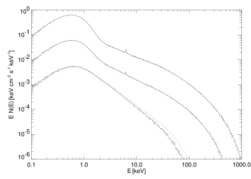
In Fig. 5, we show the spectrum of the escaping radiation for several values of the inclination angle.

Figure 5.— The spectra of escaping radiation for several values of $\mu$, where $\mu=\cos(\theta)$. The uppermost plot is the spectrum averaged over all angles. Below, in order, $\mu=0.9,0.7,0.5,0.3$, and $0.1$. For all cases, the average coronal temperature is $k\langle\mbox{$T_{\mbox{\scriptsize\sc c}}$}\rangle=118$ keV, the optical depth is $\mbox{$\tau_{\mbox{\scriptsize\sc t}}$}=0.25$, and the black-body temperature of the disk is $k\mbox{$T_{\mbox{\scriptsize\sc bb}}$}=200$ eV.

We define $\mu=\cos(\theta)$, where $\theta$ is the angle between the line of sight and the normal of the accretion disk. As expected, the spectral shape does not vary with respect to the inclination angle for optically thick models. However, for optically thin models, the spectral shape of the escaping radiation field (and the internal radiation field) does vary with $\mu$. Since the effective optical depth for radiation leaving the accretion disk is $\tau/\mu$, the fraction of black-body radiation that escapes the system without subsequent interactions with the coronane

decreases with decreasing $\mu$. Consequently, the thermal-excess gets weaker with decreasing values of $\mu$ (These arguments also apply to the strength of the Fe K$\alpha$ fluorescence line). Finally, the spectrum becomes softer as $\mu$ decreases since the magnitude of the reflection ‘hump’ decreases with the effective optical depth. These results are in agreement with HM93. Therefore, the spectra of ADCs that are seen ‘face-on’ ($\mu=1$) are the hardest, but they also have the largest amount of thermal excess. On the other hand, ADCs viewed “edge on” do not have an observationally recognizable soft-excess in their spectra, nor do they contain any reprocessing features. If the matter responsible for producing the “reflection features” is the optically thick, cold accretion disk that is also producing the seed photons, it does not appear possible that the spectra of ADCs can have strong reflection features without also containing a strong soft excess. While a very cold accretion disk (i.e., $k\mbox{$T_{\mbox{\scriptsize\sc bb}}$}\lesssim 10$ eV) would produce thermal emission that could be “hidden” due to the efficient Galactic absorption of UV radiation, it is questionable whether an accretion disk of a BHC, in the radial region where most of the seed-photons are produced, could be so cold (For a more detailed discussion, see paper II).

5.5. Strength of Fe K$\alpha$ Fluorescence Line

The strength of the Fe K$\alpha$ fluorescence line for BHCs provides stringent constraints on the properties of ADC models. For a slab geometry, roughly half of the Comptonized radiation field within the corona is reprocessed within the cold accretion disk. For parameters appropriate for BHCs, where the radiation field is hard (having a photon index of $\Gamma\sim 1.5$), the large amount of reprocessing gives rise to a very large equivalent width (EW) of the Fe K$\alpha$ line. For optically thin models having a temperature $130\geq k\mbox{$T_{\mbox{\scriptsize\sc c}}$}\geq 100$ keV  the angle-averaged EW of the iron line is $120\,\mbox{e\kern-0.99585pt{V}}\geq{\rm EW}\geq 90\,\mbox{e\kern-0.99585pt{V}}$ (for each temperature, there is a scatter of about $10$ eV due to the range of optical depths, the uncertainty in the EW measurements, and the statistical nature of the Monte Carlo simulations). The predicted EWs would be even higher than these values if a harder spectrum (i.e. a spectral shape that describes the Cyg X-1 observations better than the self-consistent spectrum) were incident onto the cold accretion disk. For example, according to simulations with our linear Monte Carlo code, a radiation field with a power-law index of 1.5 and an exponential cutoff at 150 keV irradiated onto the cold disk will result in an EW $\sim 150$ eV for a ‘face-on’ orientation. Although there is a great deal of uncertainty, the observed EW of the Fe K$\alpha$ line of BHCs is very small, usually having only an upper limit rather than a true detection. For Cyg X-1, the EW is $\lesssim 70$ eV (Ebisawa et al. (1996); Gierliński et al. (1997)). Therefore, unless the abundance of iron is much less than solar, the slab geometry models predict EW values that are significantly larger than the values observed for Cyg X-1. As we discuss in paper II, this problem is not encountered with models having a sphere$+$disk geometry. For that geometry, the accretion disk, as seen by the corona, has a covering factor roughly least one third of that for the slab geometry, giving rise to less reprocessing of coronal radiation (Done et al. (1992)).

5.6. Comparisons to Previous Models

5.6.1 Hua & Titarchuk (1995)

The major difference between our models and the analytic models of Sunyaev & Titarchuk (1980) and Hua & Titarchuk (1995) is that our models take into account the reprocessing of radiation within the cold accretion disk, which gives rise to reflection features in the spectra. In addition, our models give a more accurate description of the transition between the thermal black-body (seed photons) and the Comptonized portion of the spectrum since Titarchuk’s analytical model is only valid for energies much higher than the energy of the seed photons (nor does this model include any anisotropic effects). Therefore, it is expected that they will predict different spectra of escaping radiation. However, due to the popularity of this model, we give a comparison (Fig. 6) of our models to the XSPEC version of Titarchuk’s slab-geometry Comptonization model (Hua & Titarchuk (1995)).

Figure 6.— Comparison of the predicted spectrum of escaping radiation with the analytic model of Titarchuk (Hua & Titarchuk (1995)), for several inclination angles. Solid lines correspond to our model, and the hashed lines correspond to Titarchuk’s model. From top to bottom, $\mu=$ 0.1, 0.5, and 0.9. Again, $k\langle\mbox{$T_{\mbox{\scriptsize\sc c}}$}\rangle=118$ keV, $\mbox{$\tau_{\mbox{\scriptsize\sc t}}$}=0.25$, and $k\mbox{$T_{\mbox{\scriptsize\sc bb}}$}=200$ eV.

Here, the spectral shape of the seed photons for Titarchuk’s model is described by a Wien law rather than a Planckian distribution. Although the two models differ significantly, they do agree for energies much higher than $k\mbox{$T_{\mbox{\scriptsize\sc bb}}$}$ if the reflection features are ignored. However, our high-energy tails do not decrease with increasing energy as rapidly as the analytic model. This disagreement has been discussed by several other authors (Stern et al. (1995a) and Skibo et al. (1995)). We also note that, with the current implementation of XSPEC (version 9.0), it is not possible to add a reflection component to Titarchuk’s Comptonization model self-consistently.

5.6.2 Power-Law with Exponential Cutoff

As shown in Fig. 7a, we have attempted to describe our simulated spectra of escaping radiation by a power-law with an exponential cut-off,

$$N_{\rm E}=F_{\rm 0}E^{-\Gamma}\exp(-E/E_{\rm 0}),$$ (9)

where $N_{\rm E}$ is the photon flux as a function of energy, $E$.

Figure 7.— Comparison of the predicted spectrum of escaping radiation with spectra of the form $F(E)\propto E^{-\Gamma}\exp(-E/E_{\rm cut})$. (a) The uppermost spectrum is the angle-averaged spectrum; then, from top to bottom, $\mu=$ 0.1, 0.3, 0.5, 0.7, and 0.9. The model parameters are the same as in Fig. 6. (b) The residuals of the numerical model divided by the analytical model for $\mu=0.9$.

Although we were able to achieve good ‘by-eye’ fits for the angle-averaged spectrum (integrated over all values of $\mu$), we were unable to find good fits for individual bins of $\mu$. This problem is due to the presence of reflection features. In Fig. 7b we show the residuals of our numerical model divided by the analytical model (equation 9) for $\mu=0.1$. The fits become better as the inclination angle increases since the strength of reprocessing features decreases with increasing angles (§ 5.4.2). It appears to be a coincidence that, for the angle-averaged spectrum, the reflection features add up in such a way that a power-law is better preserved.

5.6.3 Reflected Exponentially Cutoff Power-law

Using XSPEC, we have compared our model to the reflected exponentially cutoff power-law model pexrav (Magdziarz & Zdziarski (1995)). Using the RXTE PCA response matrix, we simulated a $10^{4}$ second observation using fakeit and our NLMC model, where $k\mbox{$T_{\mbox{\scriptsize\sc bb}}$}=200$ eV, $k\langle\mbox{$T_{\mbox{\scriptsize\sc c}}$}\rangle=118$ keV, $\mbox{$\tau_{\mbox{\scriptsize\sc t}}$}=0.25$, and $\mu=0.9$. As shown in Fig. 8, We fit these ‘data’ with a superposition of a $200$ eV blackbody, a Gaussian line at $6.4$ keV, and pexrav. Our best fit yielded a photon index of $2.0$, a cutoff energy $E_{\rm c}=400$ keV, and the relative reflection parameter $f=0.48$.

Figure 8.— Comparison of the reflected exponentially cutoff power-law model, pexrav (Magdziarz & Zdziarski (1995)), to the NLMC model. Using XSPEC (Arnaud (1996)), “fake” data was produced by folding the NLMC model through the RXTE PCA response matrix. The parameters of the NLMC model are the same as in Fig. 6. A Gaussian at $6.4$ keV and a blackbody distribution with $k\mbox{$T_{\mbox{\scriptsize\sc bb}}$}=200$ eV have been added to the pexrav model. In the pexrav model, an isotropic radiation field given by $N(E)\propto E^{-\Gamma}\exp[-E/E_{c}]$ is reflected by a slab of cold matter. The “best-fit” reflection model resulted in an equivalent width of the Fe K$\alpha$ line $EW\approx 100$ eV, $\Gamma\approx 2.0$, $E_{\rm c}=400$ keV, and the covering fraction of the disk $f=0.48$. Galactic absorption has been taken into account by both models using wabs (using the Morrison and McCammon cross-sections) and assuming $N_{\rm H}=6\times 10^{21}$ cm^-2.

We froze the abundance parameter to unity, and set $\mu=0.9$. It is clear that there is much more structure in our NLMC model than in the reflection model, showing a pitfall of assuming that a Comptonized, un-reflected spectrum can be described by an exponentially cutoff power-law. It is also interesting that the best fit covering fraction is $f<0.5$ given that the physical covering fraction for the slab geometry is $f=1$.

6. Conclusions

We present accretion disk corona models where the radiation field, the temperature, and the total opacity of the corona are determined self-consistently. We take into account the coupling between the corona and the accretion disk by including reprocessing of radiation in the accretion disk.

The range of self-consistent temperatures and total opacities places severe limitations on the model’s applicability in explaining the X-ray spectra of BHCs. The maximum corona temperature for models having $\mbox{$\tau_{\mbox{\scriptsize\sc t}}$}>0.3$ is $k\mbox{$T_{\mbox{\scriptsize\sc c}}$}\approx 110$ keV. The corresponding angel-averaged, $5$ keV - $30$ keV photon index is $\Gamma\gtrsim 1.8$, a value too large to explain the observed hard spectra of BHCs (with typical photon power-law indices of $\sim 1.5$). Even models with a ‘face-on’ orientation predict photon indeces of $\Gamma\gtrsim 1.7$. The spectra (for energies $E\gtrsim 5$ keV) of BHCs, most notably Cyg X-1, have been adaquately described by linear ADC models where $\tau\sim 0.3-0.5$ and $kT\sim 150$ keV (e.g. Haardt et al. (1993); Titarchuk (1994)). All of these previous ADC models are not self-consistent, for they used temperature and opacity values that are outside the allowed region.

In addition, as described in paper II, attempts to describe the broad-band spectrum of Cyg X-1 have proven to be much more difficult than modeling the spectrum over a smaller energy range. This difficulty is due to the fact that optically thin ADC models always predict a very large thermal excess, a feature not found in the observations, unless the inclination angle is nearly ‘edge-on.’ For the case of Cyg X-1, these high inclination angles probably can be ruled out since it appears that the inclination angle is between 32^∘ and 40^∘ (Ninkov, Walker, & Yang, 1987). Additionally, models with edge-on orientations predict that no reprocessing or reflection features will be present in the spectra. Optically thick models, which also predict a small thermal excess, have a self-consistent coronal temperature that is much too cold to explain the spectra of BHCs. Due to galactic absorption, the predicted thermal excess decreases with decreasing values of the black-body temperature. However, a colder accretion disk results in a higher Compton cooling rate, yielding even lower coronal temperatures than the values corresponding to a 200 eV disk.

References

- Arnaud (1996) Arnaud, K. A., 1996, in: Jacoby, G. H., Barnes, J., eds, Astronomical Data Analysis Software and Systems V, ASP Conf. Series Vol 101, San Francisco, p. 17
- Akhiezer & Berestetskii (1965) Akhiezer, A. I., Berestetskii, V. B., 1965, Quantum Electrodynamics, New York: Interscience
- Balbus & Hawley (1991) Balbus, S. A., Hawley, J. F., 1991, ApJ, 376, 214
- Balbus et al. (1996) Balbus, S. A., Hawley, J. F., Stone, J. M., 1996, ApJ, 467, 76
- Band et al. (1990) Band, I. M., Trzhaskovskaya, M. B., Verner, D. A., Yakovlev, D. G., 1990, A&A, 237, 267
- Biémont et al. (1991) Biémont, et al., 1991, A&A, 249, 539
- Chen (1995) Chen, X., 1995, ApJ, 448, 803
- Coppi (1992) Coppi, P. S., 1992, MNRAS, 258, 657
- Done et al. (1992) Done, C., Mulchaey, J. S., Mushotzky, R. F., Arnaud, K. A., 1992, ApJ, 395, 275
- Dove et al. (1997) Dove, J. B., Wilms, J., Maisack, M. G., Begelman, M. C., 1997, ApJ, submitted (paper II)
- Ebisawa et al. (1996) Ebisawa, K., et al., 1996, ApJ, 467, 419
- Fabian (1994) Fabian, A. C., 1994, ApJS, 92, 555
- Galeev et al. (1979) Galeev, A. A., Rosner, R., Vaiana, G. S., 1979, ApJ, 229, 318
- George & Fabian (1991) George, I. M., Fabian, A. C., 1991, MNRAS, 249, 352
- Gierliński et al. (1997) Gierliński, M., Zdziarski, A. A., Done, C., Johnson, W. N., Ebisawa, K., Ueda, Y., Haardt, F., Phlips, B. F., 1997, MNRAS, in press
- Gilfanov et al. (1993) Gilfanov, M., et al., 1993, A&AS, 97, 303
- Górecki & Wilczewski (1984) Górecki, A., Wilczewski, W., 1984, Acta Astron., 34, 141
- Grebenev et al. (1993) Grebenev, S., et al., 1993, A&AS, 97, 281
- Grevesse & Anders (1989) Grevesse, N., Anders, E., 1989, in Cosmic abundances of matter, ed. C. WaddingtonAIP Conf. Proc. 183, New York: AIP, 1
- Guilbert & Rees (1988) Guilbert, P. W., Rees, M. J., 1988, MNRAS, 233, 475
- Haardt (1993) Haardt, F., 1993, ApJ, 413, 680, H93
- Haardt et al. (1993) Haardt, F., Done, C., Matt, G., Fabian, A. C., 1993, ApJ, 411, L95
- Haardt & Maraschi (1991) Haardt, F., Maraschi, L., 1991, ApJ, 380, L51, HM91
- Haardt & Maraschi (1993) Haardt, F., Maraschi, L., 1993, ApJ, 413, 507, HM93
- Haardt et al. (1994) Haardt, F., Maraschi, L., Ghisellini, G., 1994, ApJ, 432, L95
- Haardt et al. (1997) Haardt, F., Maraschi, L., Ghisellini, G., 1997, ApJ, 476, 620
- Hawley et al. (1996) Hawley, J. C., et al., 1996, in Accretion Phenomena and Related Outflows, IAU Coll. 163, in press
- Hawley et al. (1994) Hawley, J. F., Gammie, C. F., Balbus, S. A., 1994, in The First Stromlo Symposium: The Physics of Active Galaxies, ed. G. V. Bicknell, M. A. Dopita, P. J. Quinn, ASP Conf. Series, 54, San Francisco: Astron. Soc. of the Pacific, 53
- Holweger et al. (1991) Holweger, H., Bard, A., Kock, A., Kock, M., 1991, A&A, 249, 545
- Hua & Titarchuk (1995) Hua, X. M., Titarchuk, L., 1995, ApJ, 449, 188
- Kaastra & Mewe (1993) Kaastra, J. S., Mewe, R., 1993, A&AS, 97, 443
- Kusunose & Mineshige (1995) Kusunose, M., Mineshige, S., 1995, ApJ, 440, 100
- Lightman & Rybicki (1980) Lightman, A. P., Rybicki, G. B., 1980, ApJ, 236, 928
- Lightman & Zdziarski (1987) Lightman, A. P., Zdziarski, A. A., 1987, ApJ, 319, 643
- Luo & Liang (1994) Luo, C., Liang, E. P., 1994, MNRAS, 266, 386
- Magdziarz & Zdziarski (1995) Magdziarz, P., Zdziarski, A., 1995, MNRAS, 273, 837
- Maisack et al. (1993) Maisack, M., et al., 1993, ApJ, 407, L61
- Nakamura & Osaki (1993) Nakamura, K., Osaki, Y., 1993, PASJ, 45, 775
- Nandra et al. (1991) Nandra, K., et al., 1991, MNRAS, 248, 760
- Narayan & Yi (1995) Narayan, R., Yi, I., 1995, ApJ, 452, 710
- Ninkov et al. (1987) Ninkov, Z., Walker, G. A. H., Yang, S., 1987, ApJ, 321, 425
- Pounds et al. (1990) Pounds, et al., 1990, Nat, 344, 132
- Poutanen & Svensson (1996) Poutanen, J., Svensson, R., 1996, ApJ, 470, 249
- Pozdnyakov et al. (1983) Pozdnyakov, L. A., Sobol’, I. M., Sunyaev, R. A., 1983, Astrophys. Sp. Phys. Rev., 2, 189
- Shapiro & Lightman (1976) Shapiro, S. L., Lightman, A. P., 1976, ApJ, 204, 187
- Skibo et al. (1995) Skibo, J. G., Dermer, C. D., Ramaty, R., McKinley, J., 1995, ApJ, 446, 86
- Stern et al. (1995a) Stern, B., Begelman, M. C., Sikora, M., Svensson, R., 1995a, MNRAS, 272, 291
- Stern et al. (1995b) Stern, B., et al., 1995b, ApJ, 449, L13
- Stern (1985) Stern, B. E., 1985, SvA, 29, 306
- Stern (1988) Stern, B. E., 1988, The Large Particle Method, Technical Report 88/51 A, Nordita
- Stone et al. (1996) Stone, J. M., Hawley, J. F., Gammie, C. F., Balbus, S. A., 1996, ApJ, 463, 656
- Sunyaev & Titarchuk (1980) Sunyaev, R. A., Titarchuk, L. G., 1980, A&A, 86, 121
- Sunyaev & Titarchuk (1985) Sunyaev, R. A., Titarchuk, L. G., 1985, A&A, 143, 374
- Svensson (1987) Svensson, R., 1987, MNRAS, 227, 403
- Titarchuk (1994) Titarchuk, L., 1994, ApJ, 434, 570
- Tout & Pringle (1992) Tout, C., Pringle, J., 1992, MNRAS, 259, 604
- Verner et al. (1993) Verner, D. A., Yakovlev, D. G., Band, I. M., Trzhaskovskaya, M. B., 1993, At. Data Nucl. Data Tables, 55, 233
- White & Lightman (1990) White, T. R., Lightman, A. P., 1990, ApJ, 352, 495
- Wilms et al. (1997) Wilms, J., Dove, J. B., Maisack, M., Staubert, R., 1997, A&AS, 120, C159
- Zdziarski (1985) Zdziarski, A. A., 1985, ApJ, 289, 514