1 Introduction

The observed cosmic microwave background (CMB) radiation provides strong evidence for the hot big bang. The success of primordial nucleosynthesis calculations (“Big-bang nucleosynthesis”) requires a cosmic background radiation (CBR) characterized by a temperature $kT\sim 1\,$MeV at a redshift of $z\simeq 10^{9}$. In their pioneering work, Gamow, Alpher, and Herman[2] realized this and predicted the existence of a faint residual relic of the primordial radiation, with a present temperature of a few degrees. The observed CMB is interpreted as the current manifestation of the hypothesized CBR.

The CMB was serendipitously discovered by Penzias and Wilson[45] in 1964. Its spectrum is well characterized by a $2.73\pm 0.01\,$K black-body (Planckian) spectrum over more than three decades in frequency (see Figure 1) A non-interacting Planckian distribution of temperature $T_{i}$ at redshift $z_{i}$ transforms with the universal expansion to another Planckian distribution at redshift $z_{r}$ with temperature $T_{r}/(1+z_{r})=T_{i}/(1+z_{i})$. Hence thermal equilibrium, once established (e.g. at the nucleosynthesis epoch), is preserved by the expansion, in spite of the fact that photons decoupled from matter at early times. Because there are about $10^{9}$ photons per nucleon, the transition from the ionized primordial plasma to neutral atoms at $z\sim 1000$ does not significantly alter the CBR spectrum[44].

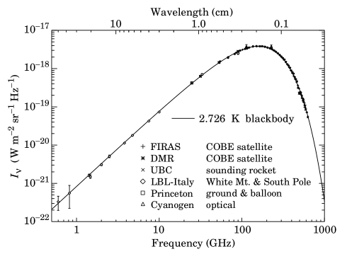
Figure 1.  : Precise measurements of the CMB spectrum. The line represents a 2.73 K blackbody, which describes the spectrum very well, especially around the peak of intensity. The spectrum is less well constrained at frequencies of 3 GHz and below ($10\,$cm and longer wavelengths). (References for this figure are at the end of this section under “CMB Spectrum References.”)

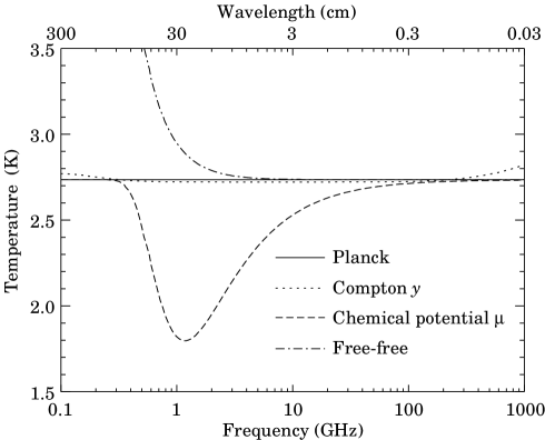
Figure 2.  : The shapes of expected, but so far unobserved, CMB distortions, resulting from energy-releasing processes at different epochs.

2 Theoretical spectral distortions

The remarkable precision with which the CMB spectrum is fitted by a Planckian distribution provides limits on possible energy releases in the early Universe, at roughly the fractional level of $10^{-4}$ of the CBR energy, for redshifts ${}_{\sim}^{<}10^{7}$ (corresponding to epochs ${}_{\sim}^{>}1\,$year). The following three important classes of spectral distortions (see Figure 2 generally correspond to energy releases at different epochs. The distortion results from interactions with a hot electron gas at temperature $T_{e}$.

2.1 Compton distortion

Late energy release ($z\sim 10^{5}$). Compton scattering ($\gamma e\rightarrow\gamma^{\prime}e^{\prime}$) of the CBR photons by a hot electron gas creates spectral distortions by transferring energy from the electrons to the photons. Compton scattering cannot achieve thermal equilibrium for $y<1$, where

$$y=\int^{z}_{0}~{}\frac{kT_{e}(z^{\prime})-kT_{\gamma}(z^{\prime})}{m_{e}c^{2}}\;\sigma_{T}\;n_{e}(z^{\prime})\;c\;\frac{dt}{dz^{\prime}}\;dz^{\prime}{\rm~{},}$$ (1)

is the integral of the number of interactions, $\sigma_{T}\;n_{e}(z)\;c\;dt$, times the mean-fractional photon-energy change per collision[54]. For $T_{e}\gg T_{\gamma}$ $y$ is also proportional to the integral of the electron pressure $n_{e}kT_{e}$ along the line of sight. For standard thermal histories $y<1$ for epochs later than $z\simeq 10^{5}$.

The resulting CMB distortion is approximately a temperature decrement

$$\Delta T_{\rm RJ}=-2y\;T_{\gamma}$$ (2)

in the Rayleigh-Jeans ($h\nu/kT_{\gamma}\ll 1$) portion of the spectrum, and a rapid rise in temperature in the Wien ($h\nu/kT_{\gamma}\gg 1$) region, i.e. photons are shifted from low to high frequencies. The magnitude of the distortion is related to the total energy transfer[54] $\Delta E$ by

$$\Delta E/E_{\rm CBR}=e^{4y}-1\simeq 4y{\rm~{}.}$$ (3)

A prime candidate for producing a Comptonized spectrum is a hot intergalactic medium. A hot ($T_{e}>10^{5}\,$K) medium in clusters of galaxies also produces a partially Comptonized spectrum as seen through the cluster, known as the Sunyaev-Zel’dovich effect. Based upon X-ray data, the predicted large angular scale total combined effect of the hot intracluster medium should produce $y<10^{-6}$[6].

2.2 Bose-Einstein or chemical potential distortion

Early energy release ($z\sim 10^{5}$–$10^{7}$). After many Compton scatterings ($y>1$), the photons and electrons will reach statistical (not thermodynamic) equilibrium, because Compton scattering conserves photon number. This equilibrium is described by the Bose-Einstein distribution with non-zero chemical potential:

$$n=\frac{1}{e^{x+\mu_{0}}-1}{\rm~{},}$$ (4)

where $x\equiv{h\nu/kT}$ and $\mu_{0}\simeq 1.4{\Delta E}/E_{\rm CBR}$, with $\mu_{0}$ being the dimensionless chemical potential that is required to conserve photon number.

The collisions of electrons with nuclei in the plasma produce free-free (thermal bremsstrahlung) radiation: $eZ\rightarrow eZ\gamma$. Free-free emission thermalizes the spectrum to the plasma temperature at long wavelengths. Including this effect, the chemical potential becomes frequency-dependent,

$$\mu(x)=\mu_{0}e^{-2x_{b}/x}{\rm~{},}$$ (5)

where $x_{b}$ is the dimensionless transition frequency at which Compton scattering of photons to higher frequencies is balanced by free-free creation of new photons. The resulting spectrum has a sharp drop in brightness temperature at centimeter wavelengths[5]. The minimum wavelength is determined by $\Omega_{B}$.

The equilibrium Bose-Einstein distribution results from the oldest non-equilibrium processes $(10^{5}<z<10^{7})$, such as the decay of relic particles or primordial inhomogeneities. Note that free-free emission (thermal bremsstrahlung) and radiative-Compton scattering effectively erase any distortions[9][53],[13] to a Planckian spectrum for epochs earlier than $z\sim 10^{7}$.

Figure 3.  : Upper Limits (95% CL) on fractional energy ($\Delta E/E_{\rm CBR}$) releases as set by lack of CMB spectral distortions resulting from processes at different epochs. These can be translated into constraints on the mass, lifetime and photon branching ratio of unstable relic particles, with some additional dependence on cosmological parameters such as $\Omega_{B}$ [55][21].

2.3 Free-free distortion

Very late energy release ($z\ll 10^{3}$). Free-free emission from recent reionization $(z<10^{3})$ and from a warm intergalactic medium can create rather than erase spectral distortion in the late universe. The distortion arises because of the lack of Comptonization at recent epochs. The effect on the present-day CMB spectrum is described by

$$\Delta T_{f\!f}=T_{\gamma}\;{Y_{f\!f}}/{x^{2}},$$ (6)

where $T_{\gamma}$ is the undistorted photon temperature, $x$ is the dimensionless frequency, and $Y_{f\!f}/x^{2}$ is the optical depth to free-free emission:

$$Y_{f\!f}=\int^{z}_{0}~{}\frac{T_{e}(z^{\prime})-T_{\gamma}(z^{\prime})}{T_{e}(z^{\prime})}\frac{8\pi e^{6}h^{2}n_{e}^{2}\;g}{3m_{e}(kT_{\gamma})^{3}\;\sqrt{6\pi\,m_{e}\,kT_{e}}}\;\frac{dt}{dz^{\prime}}dz^{\prime}{\rm~{}.}$$ (7)

Here $h$ is Planck’s constant, $n_{e}$ is the electron density and $g$ is the Gaunt factor[3].

3 Spectrum Observations

Beginning with the original discovery of the CMB by Penzias and Wilson there was a rush of observations in the period 1965 through 1967. For the most part interest shifted to the short-wavelength (high-frequency) portion of the spectrum to observe the peak and Wien turn down to show that the spectrum was thermal. In the early 1980’s effort was renewed for observing the low frequency (Rayleigh-Jeans) region primarily by a USA-Italian collaboration consisting of my group (LBNL-Berkeley), Bruce Partridge (Haverford), Reno Mandolesi’s group (Bologna), and Giorgio Sironi’s group (Milano) with theoretical support from Luigi Danese and Gianfranco DeZotti (Padua). We determined that scientific goals and technology had advanced to the point that the long wavelength ($>$ 1 cm) region should and could be measured more accurately.

The general experimental concept is to observe the total power coming from the sky and compare that to a well known reference source using specially designed radio receivers called radiometers. The references we used were carefully designed blackbodies with total temperature of about 3.8 K which was very close to the total sky signal so that the gain calibration of our radiometers was not a critical component of the observation. The sky signal is the sum of many terms

$$T_{sky}=T_{CMB}+T_{atmosphere}+T_{Galaxy}+T_{Sun/Moon}+T_{instrum}+T_{terrestial}$$ (8)

The total sky signal is dominated by the CMB, $T_{CMB}=2.73$ K, and the atmospheric emission, $T_{atmosphere}\approx 1$ K. The other terms are generally much smaller giving a total sky signal close to 3.8 K of total power which closely matches the absolute reference load. (At very low frequencies the Galactic signal tends to be greater but the atmospheric component decreases.)

The signal from the atmosphere is determined by scanning the radiometer beam through various zenith angles and thus varying the air mass observed and the data are then constrained by continuity and comparison to an atmospheric model.

Our groups carried out a series of measurements from the high, dry sites at White Mountain University of California Research Station (3800 meters) which is in the rain shadow of the Sierras and the NSF South Pole Station. Table 4 at the end of the text (since it is so large) gives a summary of the low-frequency observations and observations excluding those from COBE FIRAS and the UBC rocket borne experiment which are in separate tables.

3.1 Interstellar Molecules and Atomic Systems

Observations of interstellar molecules and atomic systems, most especially cyanogen (CN), provide a probe of the CMB temperature in narrow wavelength bands at remote locations. CN has proved most used and most precise as the observations are made at optical wavelengths and use well-developed technology. They are by their nature indirect observations in that what is measured is the relative population of various energy levels and the ratio can be used to estimate $T_{CMB}$. Thus one is observing the total excitation of the system and accounting must be done to subtract the contribution of other potential sources. Fortunately, for cold, non-dense clouds, the contribution from sources other than the CMB tends to be quite small, typically on the order of 0.1 K compared to 2.73 K.

CN molecules existence abundantly in interstellar clouds. If a cloud lies along the line of sight from a bright optical source, the CN produces narrow absorption lines features on the source spectrum. These absorbtion lines were detected in 1941 (more than half a century ago and 23 years before the CMB was discovered by Penzias and Wilson) by Adams [1], McKellar [34], and others and were noted as a puzzle. McKellar estimated a value for the excitation temperature of the CN of a few degrees. Immediately after the CMB discovery many people began observations of CN systems for information about the CMB temperature. Those efforts have continued to the present and the most recent results are shown in the following table along with some results for other molecules. Note that there is a discrepancy of results on CN between [41] and [50].

TABLE 1.  : Recent Molecular Measurements of $T_{CMB}$

 Reference Molecule Wavelength Temperature (Year) (mm) (K)  Meyer & Jura (1985) CN 2.64 $2.70\pm 0.04$ K Meyer et al. (1989) CN 2.64 $2.75\pm 0.03$ K Meyer et al. (1989) CN 2.64 $2.77\pm 0.07$ K Meyer et al. (1989) CN 2.64 $2.75\pm 0.08$ K Meyer & Jura (1985) CN 1.32 $2.76\pm 0.20$ K Meyer et al. (1989) CN 1.32 $2.83\pm 0.09$ K Meyer et al. (1989) CN 1.32 $2.85\pm 0.16$ K Crane et al. (1986) CN 2.64 $2.74\pm 0.05$ K Crane et al. (1989) CN 2.64 $2.796^{+0.014}_{-0.039}$ K Palazzi et al.(1990) CN 1.32 $2.83\pm 0.07$ K Palazzi et al.(1990) CN 1.32 $2.82\pm 0.11$ K Kaiser & Wright (1990) CN 2.64 $2.75\pm 0.04$ K Palazzi et al.(1992) CN 2.64 $2.817\pm 0.02$ K Roth et al. (1993) CN 2.64 $2.729^{+0.023}_{-0.031}$ K Roth & Meyer (1995) CN 2.64 ”  Thaddeus (1972) CH 0.76 $<5.23$ K Thaddeus (1972) CH⁺ 0.36 $<7.35$ K Kogut et al. (1990) H₂CO 2.1 $3.2\pm 0.9$ K  Weighted mean $\pm 1\sigma$ $2.76\pm 0.03$ K  

3.2 COBE FIRAS

It is the measurements of the FIRAS (Far-InfraRed Absolute Spectrophotometer) on the COBE satellite that have shown definitively that the CMB spectrum is very nearly Planckian. The FIRAS instrument is a twin-input, twin-output polarizing Michelson interferometer that achieves high precision by making a differential rather than an absolute measurement.

One input is connected to view the sky through a large, low side-lobe sky horn. The other input is connected to an internal calibrator at all times. The internal calibrator is nearly a blackbody (96-98% emissivity) over the full wavelength range and is very stable. The calibrator temperature is adjusted to give nearly null interferometer output.

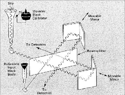
Figure 4.  : Schematic of the FIRAS instrument. There are two symmetric inputs: the power from the sky and from an internal reference blackbody. A high precision blackbody can be substituted for the sky signal input. It is a polarizing Michelson interferometer with two dihedral mirrors.

The sky horn can be filled by the external calibrator by swinging it on its pivot. The external calibrator is a re-entrant absorbing cone. The combined external calibrator and sky horn cavity is a very good blackbody with emissivity measured to be greater than 99.99% and calculated to be greater than 99.999%. The external calibrator temperature is commandable and was adjusted around null defined by the sky signal to provide an absolute and relative calibration. This operation is possible since one does not have to be concerned with windows or freezing of the atmosphere on the instrument and calibrator or with serious thermal loading.

Comparison of the signal from the sky with the signal from the external calibrator with temperature adjusted to match gives an accurate and precise measurement of deviations of the sky spectrum from a blackbody. When these small deviations are added to the calculated Planck spectrum, the FIRAS observed spectrum is produced. See Figure 5 for the measured spectrum and a 2.728 K Planckian.

Figure 5.  : The spectrum of the CMB measured by FIRAS. The error bars shown are $\pm 400\sigma$. The solid line is a 2.728 K blackbody.

The temperature of the external calibrator, when the output matches the sky viewing output, is the sky temperature. A number of small corrections must be made, e.g. to the GRT (germanium resistance thermometers) readings, cosmic ray hits, extra signal from interstellar dust or the experiment. Another method is to use the wavelength of the peak of the brightness spectrum determined by the length scale set by the dimensions of the interferometer and which is accurately checked and calibrated by the molecular lines observed in the Galactic emission by the interferometer. A third approach is to use the dipole spectrum (see dipole spectrum section) to set the temperature scale.

TABLE 2.  : COBE Measurement of $T_{CMB}$

 Method Temperature  GRT at sky match $2.730\pm 0.001$ K Peak of $\partial B_{\nu}/\partial T$ $2.726\pm 0.001$ K FIRAS Dipole Spectrum $2.717\pm 0.007$ K DMR Annual Dipole $2.725\pm 0.015$ K  Weighted mean $\pm 1\sigma$ $2.728\pm 0.002$ K  

Since the RMS deviation of the spectral intensity $I_{\nu}$ from a blackbody $B_{\nu}$ is $5\times 10^{-5}$ of the peak $B_{\nu}$ amplitude, the Planck function must be subtracted before plotting, for residuals to be seen (e.g. see Figure 6).

Figure 6.  : The residuals after subtracting a 2.728 K blackbody and the best fitted galactic emission plotted at their 95% confidence interval limit amplitudes. The distortions are shown in the same manner as the data: they are the residuals from a least squares fit to a temperature change and the best-fitted galactic emission amplitude. The solid line (G) shows the observed galactic emission and the smooth model fitting it. The curve K shows a constant intensity, $I_{\nu}$, distortion. The curve labeled $\epsilon$ shows an emissivity different from unity. The curve labeled $\mu$ shows a Bose-Einstein (chemical potential) distortion. The curve labeled $y$ shows a Compton distortion. The curve labeled “Lerner” is a fit to the 1994 FIRAS data combining the $\epsilon$ and $y$ distortions which represented an effort to have a ‘plasma’ model that explained the data; but, it is a poor fit to the improved data.

In fact the data are fitted to a form

$$I_{\nu}=B_{\nu}(T_{0})+\Delta T\frac{\partial B_{\nu}}{\partial T}+gG(\nu)$$ (9)

where $G(\nu)$ is the observed spectrum of the Galactic emission and the parameters $\Delta T$ and $g$ are adjustable to allow for a temperature correction and an unknown amount of residual Galactic emission in the darkest parts of the sky.

Using the FIRAS measured spectrum or deviations one can fit for distortions and find the results in the following table:

TABLE 3.  : FIRAS Spectral Distortion Limits

 Distortion Best Fit $\pm\sigma$ 95% CL Limit  $y$ $(-1\pm 6)\times 10^{-6}$ $1.5\times 10^{-5}$ $\mu$ $(-1\pm 4)\times 10^{-5}$ $9\times 10^{-5}$ $\epsilon-1$ $(1\pm 5)\times 10^{-5}$ $11\times 10^{-5}$ $\Delta I_{\nu}$ $(9\pm 15)$ kJy/sr 39 kJy/sr  

The first two distortions are the Compton and chemical potential distortions discussed above. The next is allowing for an emissivity different than unity. It is clear that the CMB is extremely close to the blackbody thermal spectrum. The last $\Delta I_{\nu}$ allows for an offset either from the sky or the instrument.

FIRAS also measures the spectrum of the dipole anisotropy which is shown here but is discussed in the dipole spectrum section.

Figure 7.  : The spectrum of the CMB dipole as measured by FIRAS. The solid line is the derivative of a T = 2.728 K Planck function.

Figure 8.  : The CMB dipole spectrum residuals measured by FIRAS after subtracting the derivative of the T = 2.728 K Planck function. The curve shows the best fit letting both the dipole amplitude and CMB temperature vary.

4 Spectrum summary

The CMB spectrum is consistent with a blackbody spectrum over more than three decades of frequency around the peak. A least-squares fit to all CMB measurements yields:

$T_{\gamma}=2.73\pm 0.01$ K

$n_{\gamma}=(2\zeta(3)/\pi^{2})T_{\gamma}^{3}\simeq 413\,{\rm cm^{-3}}$

$\rho_{\gamma}=(\pi^{2}/15)T_{\gamma}^{4}\simeq 4.68\times 10^{-34}\,{\rm g}\,{\rm cm^{-3}}=0.262\,{\rm eV}\,{\rm cm^{-3}}$

$|y|<1.5\times 10^{-5}$      (95% CL)

$|\mu_{0}|<9\times 10^{-5}$       (95% CL)

$|Y_{f\!f}|<1.9\times 10^{-5}$   (95% CL)

The distortion parameter limits quoted here correspond to limits [33], [4] on energetic processes $\Delta E/E_{\rm CBR}<~{}2\times 10^{-4}$ occurring between redshifts $10^{3}$ and $5\times 10^{6}$ (see Figure 3. The best-fit temperature from the COBE FIRAS experiment is $T_{\gamma}=2.728\pm 0.002\,$K[16].

5 Spectrum Interpretation & Discussion

5.1 Significance of CMB Being Planckian

Possibly the strongest arguments for the Big Bang model are the CMB’s existence and particularly its Planckian nature. This means that the CMB is both very cold and highly thermalized. Since there are roughly $10^{9}$ photons to each baryon in the Universe, it is very difficult to produce the CMB in astrophysical processes such as the absorption and re-emission of starlight by cold dust (even iron needles) or the absorption or emission by plasmas.

All alternative models and modifications to the simplest big bang model produce distortions to the CMB spectrum that have a $y$ component. It is interesting to note that any deviation from a perfectly homogeneous, isotropic, and isochronous universe causes a spectral distortion. This is a result of the fact that the sum of two blackbody spectra of different temperatures does not result in a blackbody spectrum. In the form discussed above a $y$ distortion is simply the convolution of Planckian spectra.

Thus for example, although the energy content of the CMB is comparable to that in starlight and it is possible that dust absorption, processing, and re-emission could shift the radiation frequency to this range, it is extremely unlikely that the sum of all this radiation would just match a Planckian. If somehow the dust were optically thick on cosmological scales, it is still not possible that the sum of red shifted emission from each shell would add to a Planckian for all observers. Full arguments for dust or plasma filled universes must make use of additional observations but in general there is an inconsistency with being able to see distant extragalactic sources at many wavelengths, the observed CMB spectrum, and the Copernican Principle.

Likewise, this means that for all angular scales less than the FIRAS beam size of 7^∘, rms anisotropies cannot exceed about $\Delta T/T<10^{-3}$, otherwise the superposition of temperatures would produce a $y>10^{-5}$.

5.2 Knowledge of $T_{CMB}$

The CMB temperature, $T_{CMB}$, is now known to a precision of 1%. This makes it the best known cosmological parameter. If we assume that the CMB spectrum is blackbody, we can calculate the number of photons in the CMB:

$$n_{\gamma}=(2\zeta(3)/\pi^{2})T_{\gamma}^{3}=413(T_{CMB}/2.728~{}{\rm K})^{3}\,{\rm cm^{-3}}$$ (10)

It is a small change to include simple distortions provided we know their value. We can also compute the present energy density in CMB photons

$$\rho_{\gamma}=(\pi^{2}/15)T_{\gamma}^{4}\simeq 4.68\times 10^{-34}\,{\rm g}\,{\rm cm^{-3}}=0.262\,{\rm eV}\,{\rm cm^{-3}}$$ (11)

Since the temperature scales as $T_{0}=T_{i}(1+z_{i})$, we can calculate the photon number density, $n_{\gamma i}=(1+z_{i})^{3}n_{\gamma}$, and energy density, $\rho_{\gamma i}=(1+z_{i})^{4}\rho_{\gamma}$, for any epoch $i$ with redshift $z_{i}$.

In the early universe the CBR (cosmic background radiation) which is the cosmologically redshifted present day CMB radiation dominated over the matter energy density and thus was critical to the development of the Universe. In addition most cosmological models and calculations, such as Big Bang Nucleosynthesis, are done in terms of the CBR temperature or density. In particular matter density is usually expressed in terms of the ratio either to the critical density or to the CBR density. E.g. BBNS gives the number density of baryons, $n_{b}$, as

$$n_{b}/n_{\gamma}=2.3\times 10^{-8}(\Omega_{b}h^{2})=5\times 10^{-10}h^{2}.$$ (12)

There is also the effect of the CBR/CMB on high energy cosmic rays which depends primarily on the energy density and less so on the spectrum. But the CMB implies a strong cut off of high energy protons at roughly $10^{21}$ eV due to the photoproduction of pions. Likewise, the existence of the CMB causes a cut off for high energy photons (and electrons/positrons) due to electron-positron pair production (compton scattering).

5.3 Limits on Processes in the Early Universe

There are many possible sources of energy release or augmentation from processes occurring in the early universe, including decay of primeval turbulence, elementary particles, cosmic strings, or black holes. The growth of black holes, quasars, galaxies, clusters, and superclusters might also convert energy from other forms.

Early Generation of Stars and Reionization

Wright et al.(1994a) also give limits on hydrogen burning following the decoupling. These results depend on using geometrical arguments (a $\csc|b|$ fit) to estimate the maximum amount of extragalactic energy that could have a spectrum similar to that of our own Galactic dust. We found a limit that is a factor of about 3 smaller than the polar brightness of the Milky Way. A better understanding of the Galactic dust would help produce a tighter limit on these extragalactic signals.

Consider first population III stars liberating energy that is converted by dust into far infrared light (using an optical depth of 0.02 per Hubble radius), and assume that $\Omega_{b}h^{2}=0.015$. In that case less than 0.6% of the hydrogen could have been burned after $z=80$. As a second example, consider evolving infrared galaxies as observed by the IRAS. For reasonable assumptions, we found that less than 0.8% of the hydrogen could have been burned in evolving IR galaxies.

We also obtained limits on the heating and reionization of the intergalactic medium. It does not take very much energy to reionize the intergalactic medium, relative to the CMBR energy, because there are so few baryons relative to CMBR photons. Even the strict FIRAS limits permit a single reionization event to occur as recently as $z=5$. More detailed calculations by Durrer (1993) show that the energy required to keep the intergalactic medium ionized over long periods of time is much more substantial and quite strict limits can be obtained. If the current $y$ limits were about a factor of 5 more strict, then it would be possible to test the ionization state of the IGM all the way back to the decoupling.

If the IGM were hot and dense enough to emit the diffuse X-ray background light, it should distort the spectrum of the CMBR by inverse Compton scattering. This is a special case of the Comptonization process, with small optical depth and possibly relativistic particles. Calculations show that a smooth hot IGM could have produced less than 10^-4 of the X-ray background, and that the electrons that do produce the X-ray background must also have a filling factor of less than 10^-4.

Limits on Primordial Anisotropy

Primordial perturbations will undergo energy dissipation via Silk damping. Energy released is more effective at short wavelengths where there are more oscillations. Limits on energy release are also limits on the primordial perturbation power spectrum. Hu, Scott, and Silk (1994) find an upper limit on the power spectrum index of about $n=1.55$. It is interesting that these calculations give tighter limits than existing direct measurements, even though the spectrum is only an upper limit. These results are dependent on assuming that a power law is the correct form for the fluctuations over 7 orders of magnitude of scale. There is little possibility of observational evidence to confirm this assumption over such a wide range, since small scale fluctuations have long since been replaced by nonlinear phenomena.

Limits on Shear, Vorticity, Turbulence

Limits on Gravitational Energy from LSS formation

Together, free-free and Comptonized spectra can be used to detect the onset of nuclear fusion by the first collapsed objects. Ultraviolet radiation from the first collapsed objects is expected to photoionize the intergalactic medium. Since these objects form by non-linear collapse of rare high-density peaks in the primordial density distribution, the redshift at which they form is a sensitive probe of the statistical distribution of density peaks and the matter content of the universe. Various models [56], [32] of structure formation predict significant ionization at redshifts ranging from $10<z<150$, depending on the matter content and power spectrum of density perturbations, with a “typical” value $z_{\rm ion}\approx 50$.

Limits on Particle Decay

Exotic particle decay provides another source for non-zero chemical potential. Particle physics provides a number of dark matter candidates, including massive neutrinos, photinos, axions, or other weakly interacting massive particles (WIMPs). In most of these models, the current dark matter consists of the lightest stable member of a family of related particles, produced by pair creation in the early universe. Decay of the heavier, unstable members to a photon or charged particle branch will distort the CMB spectrum provided the particle lifetime is greater than a year. Rare decays of quasi-stable particles (e.g., a small branching ratio for massive neutrino decay $\nu_{\rm heavy}\rightarrow\nu_{\rm light}+\gamma$) provide a continuous energy input, also distorting the CMB spectrum. The size and wavelength of the CMB distortion are dependent upon the decay mass difference, branching ratio, and lifetime. Stringent limits on the energy released by exotic particle decay provides an important input to high-energy theories including supersymmetry and neutrino physics[13].

Limits on Antimatter-matter mixing

In baryon symmetric cosmologies matter-antimatter annihilations gives rise to excessive distortions of the CMB spectrum [24].

Limits on Primordial Black Hole Evaporation

Only a very small fraction, $f=M_{planck}/M$, of matter can have formed black holes in the mass range $10^{11}\leq M\leq 10^{13}$ gm otherwise their evaporation in the epoch preceding recombination would have resulted in excessive distortions. For smaller blackholes the limit is much weaker, since for $M<10^{11}$ gm, evaporation would have taken place during the epoch when the photon spectrum would be completely thermalized. The constraints follow from the condition that no more than all the entropy in the universe can come from blackhole evaporation so that $f<10^{9}M_{planck}/M$.

Limits on Superconducting Cosmic Strings & Explosive Formation

If they are to play an important role in large-scale structure formation, superconducting cosmic strings would be significant energy sources, keeping the Universe ionized well past standard recombination. As a result, the energy input distorts the spectrum of the CMB but the Sunyaev-Zel’dovich effect. The Compton-$y$ parameter attains a maximum value in the range of $(1-5)\times 10^{-3}$ [39]. This is well above the observed value.

Explosive models of large-scale structure formation must create distortions in the CMB spectrum from the energy released in the shock waves. The limits on Compton-$y$ parameter rule out explosive models for structure on scales $>15$ Mpc [29].

Limits on the Variation of Fundamental Constants

Noerdlinger [38] pointed out that the intensity of the Rayleigh-Jeans portion of the CMB spectrum gives the present values of $kT$, independently of the value of the Planck constant, $h$, while the wavelength at which the spectrum peaks gives $kT$ in combination with $h$. That the two temperatures agree within errors imply that the variation of $h$ must not have exceeded a few per cent since recombination ($z\sim 1000$). Likewise a wide variety of $G$-varying cosmologies predict that the CMB spectrum will follow the standard Planckian formula multiplied by an epoch-dependent factor, which, in turn, is related to $G(t)$ [37]. The agreement between the brightness temperature in the Rayleigh-Jeans region and the temperature determined by the peak location constrain the possible variation in the gravitational constant $G$. Likewise one can obtain limits on the variation in the cosmological constant (energy density of the vacuum) [46]. The shape of the spectrum also constrains the number of large spatial dimensions (taking into account the possibility of fractal dimensions) to very nearly three ($\pm 0.02$).

6 Future Observations & Results

FIRAS has done such a splendid job of measuring the spectrum for the bulk of the CMB energy and at long wavelengths Galactic emission is such a serious foreground, it is at first difficult to imagine the motivation necessary to gather the resources for significant improvement. However, there are scientific motivations for improved measurements and there are experiments that one can envisage that may make worthwhile improvements in the observations of the CMB spectrum.

6.1 Interstellar/extragalactic Molecules & Atoms

The use of interstellar molecules, such as CN (cyanogen), offer a probe of the CMB at a remote location. There are two distinct potential scientific gains from such observations. The first is demonstrating that the CMB is universal, a thing that observations of the Sunyaev-Zeldovich effect also establishes a little more indirectly. The second is that the CMB temperature scales as $(1+z)$ with redshift. A number of indications that this might be the case exist but I would not consider them to yet be definitive (i.e. strong enough to rule out a model like the big bang). The best direct upper limit is a measurement [51] of the background temperature in high-redshift primordial clouds from an experiment aimed at measuring the primordial deuterium abundance. The claimed direct measurement [52] is based upon measuring the relative populations of hyperfine states in neutral carbon atoms observed in a gas cloud at a redshift $z=1.776$, which indicate a thermodynamic temperature of $7.4\pm 0.8$ K, which is consistent with the big-bang prediction $T(z)=(1+z)2.73~{}{\rm K}$ which is 7.58 K.

Another recent measurement by Ge et al. [18] has measured C I again in a gas cloud at a redshift $z=1.79$ with a result of $T(z=1.97)=7.9\pm 1.0$ K at 0.61 mm. Scaling by 1+z, one finds the Big Bang predicted value is 8.1 K which is again consistent. With accumulating observations and understanding of excitation mechanisms these measurements provide a definite tightening of allow region for alternative cosmologies.

6.2 ARCADE

We consider that our long wavelength ground-based observations have come near the fundamental limits set by the atmosphere and the galactic foreground. Only a very great effort or a large space-based mission is likely to generate more than a very modest improvement. At the very longest wavelengths a much better understanding of the Galactic emission is required in order to make more than just a modest improvement.

However, at intermediate wavelengths - those in the centimeter (1-6 cm), it is possible to improve the spectrum measurements significantly by balloon-borne or satellite-based experiments. It takes a large effort and very precise measurements, including careful control of systematics and very good absolute calibration, to actually improve the various limits or measurements of distortion parameters such as $\mu$ and $Y_{ff}$. But it is possible.

ARCADE (Absolute Radiometer for Cosmology, Astrophysics, and Diffuse Emission) is a balloon-borne instrument designed to make measurements of the intermediate wavelength spectrum. A conceptual schematic drawing of the instrument is shown in Figure 9.

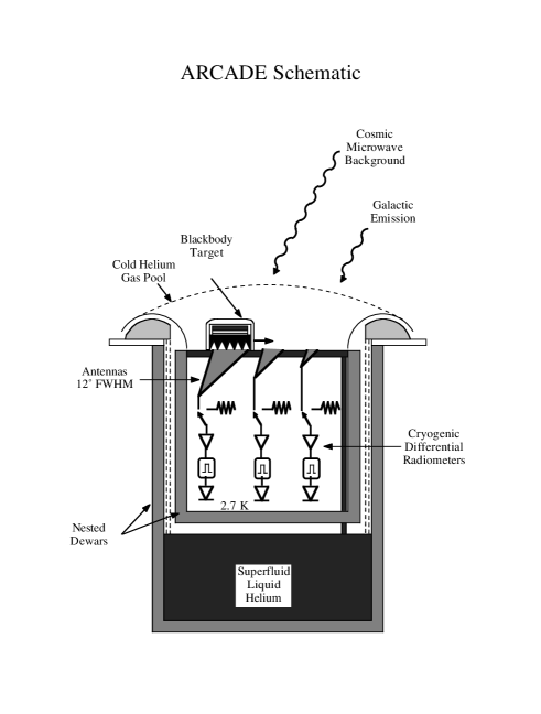
Figure 9.  : A schematic view of the ARCADE balloon-borne instrument

The instrument lives in a big bucket dewar, with a second dewar nested inside to allow the aperture plane to remain cold even through it is nearly flush with the mouth of the outer dewar. Fountain-effect pumps squirt superfluid liquid helium into a reservoir under the aperture plane assembly, where it boils to keep the top plate cold (dumping the radiative heat load from the IR lines in the atmosphere). Pinholes in the aperture plane vent the boiloff gas; a set of helium-cooled flares provide a bowl filled with a “puddle” of cold helium gas. Provided the gas is colder than 20K, it’s denser than ambient-temperature nitrogen and sits quietly as a transparent blocking layer between the cold optics and the warm atmosphere. The antennas are tipped 30 degrees with respect to the dewar symmetry axis, so that the dewar can remain upright (most of the time) while the antennas scan a circle 30 degrees in radius centered on the zenith. The dewar tips occasionally to scan various atmospheric columns, (i.e. different zenith angles to look through various amounts of atmosphere), but this will be disruptive to the absolute target performance, so this happens only part of the time. The anticipated measurement sensitivity is 1 mK from a balloon, limited by the ability to estimate/measure emission from the atmosphere, balloon, flight train, and Earth. ARCADE is basically a hardware development project for the eventual space mission. The design is kept such that the instrument can come off the balloon gondola and be put in a Spartan with minimal changes.

6.3 DIMES

The Diffuse Microwave Emission Survey (DIMES) has been selected for a mission concept study for NASA’s New Mission Concepts for Astrophysics program [28]. DIMES will measure the frequency spectrum of the cosmic microwave background and diffuse Galactic foregrounds at centimeter wavelengths to 0.1% precision (0.1 mK), and will map the angular distribution to 20 $\mu$K per 6^∘  field of view. It consists of a set of narrow-band cryogenic radiometers, each of which compares the signal from the sky to a full-aperture blackbody calibration target. All frequency channels compare the sky to the same blackbody target, with common offset and calibration, so that deviations from a blackbody spectral shape may be determined with maximum precision. Measurements of the CMB spectrum complement CMB anisotropy experiments and provide information on the early universe unobtainable in any other way; even a null detection will place important constraints on the matter content, structure, and evolution of the universe. Centimeter-wavelength measurements of the diffuse Galactic emission fill in a crucial wavelength range and test models of the heat sources, energy balance, and composition of the interstellar medium.

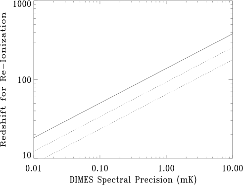
Figure 10.  : Upper limits to the redshift $z_{\rm ion}$ at which the intergalactic medium (IGM) becomes reionized, as a function of the DIMES spectral precision. The cosmologically interesting region $z_{\rm ion}<100$ requires precision 0.1 mK or better.

The FIRAS measurement at sub-mm wavelengths shows no evidence for Compton heating from a hot IGM. Since the Compton parameter $y\propto n_{e}T_{e}$, the IGM at high redshift must not be very hot ($T_{e}\sim 10^{5}$ K) or reionization must occur relatively recently ($z_{\rm ion}<10$). DIMES provides a definitive test of these alternatives. Since the free-free distortion $Y_{\rm ff}\propto n_{e}^{2}/\sqrt{T_{e}}$, lowering the electron temperature increases the spectral distortion [3]. Figure 10 shows the limit to $z_{\rm ion}$ that could be established from the combined DIMES and FIRAS spectra, as a function of the DIMES sensitivity. A spectral measurement at centimeter wavelengths with 0.1 mK precision can detect the free-free signature from the ionized IGM, allowing direct detection of the onset of hydrogen burning.

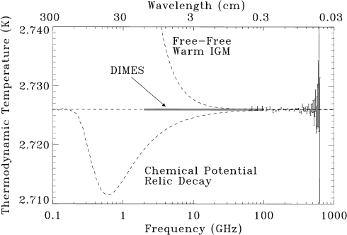
Figure 11.  : Current 95% confidence upper limits to distorted CMB spectra. The FIRAS data and DIMES 0.1 mK error box are also shown; error bars from existing cm-wavelength measurements are larger than the figure height. An absence of distortions at millimeter and sub-mm wavelengths does not imply correspondingly small distortions at centimeter wavelengths.

DIMES also provides a sensitive test for early energy releases, such as the decay of exotic heavy particles or metric perturbations from GUT and Planck-era physics.

DIMES will provide a substantial increase in sensitivity for non-zero chemical potential (Figure 11). Such a distortion arises naturally in several models. The COBE anisotropy data are well-described [20] by a Gaussian primordial density field with power spectrum $P(k)\propto k^{n}$ per comoving wave number $k$, with power-law index $n=1.2\pm 0.3$. Short-wavelength fluctuations which enter the horizon while the universe is radiation-dominated oscillate as acoustic waves of constant amplitude and are damped by photon diffusion, transferring energy from the acoustic waves to the CMB spectrum and creating a non-zero chemical potential [10], [23]. The energy transferred, and hence the magnitude of the present distortion to the CMB spectrum, depends on the amplitude of the perturbations as they enter the horizon through the power-law index $n$. Models with “tilted” spectra $n>1$ produce observable distortions.

Galactic Astrophysics

Measurements of the diffuse sky intensity at centimeter wavelengths also provide valuable information on astrophysical processes within our Galaxy. Figure 12 shows the relative intensity of cosmic and Galactic emission at high galactic latitudes. Diffuse Galactic emission at centimeter wavelengths is dominated by three components: synchrotron radiation from cosmic-ray electrons, electron-ion bremsstrahlung (free-free emission) from the warm ionized interstellar medium (WIM), and thermal radiation from interstellar dust. Despite surveys carried out over many years, relatively little is known about the physical conditions responsible for these diffuse emissions. Precise measurements of the diffuse sky intensity over a large fraction of the sky, calibrated to a common standard, will provide answers to outstanding questions on physical conditions in the interstellar medium (ISM):

$\bullet$ What is the heating mechanism in the ISM? Is the diffuse gas heated by photoionization from the stellar disk, shocks, Galactic fountain flows, or decaying halo dark matter?

$\bullet$ How are cosmic rays accelerated? Is the energy spectrum of local cosmic-ray electrons representative of the Galaxy as a whole?

$\bullet$ What is the shape, constitution, and size distribution of interstellar dust? Is there a distinct “cold” component in the cirrus?

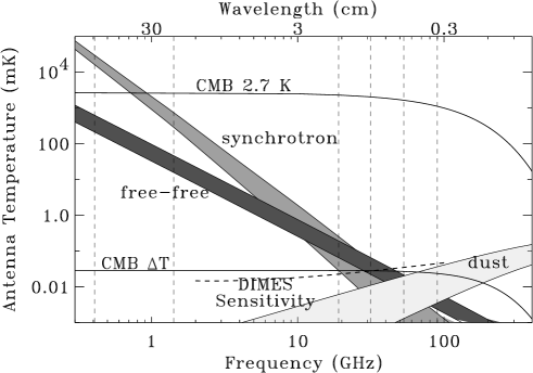
Figure 12.  : CMB and Galactic emission spectra. The shaded regions indicate the signal range at high latitude ($|b|>30^{\circ}$) and include the effects of spatial structure and uncertainties in the spectral index of the Galactic emission components. Solid lines indicate the mean CMB spectrum and rms amplitude of anisotropy. Vertical dashed lines indicate existing sky surveys. The DIMES sensitivity for a 6-month mission is shown.

The Galactic radio foregrounds may be separated from the CMB by their frequency dependence and spatial morphology. DIMES will map radio free-free emission from the warm ionized interstellar medium. The ratio of radio free-free emission to H$\alpha$ emission will map the temperature of the WIM to 20% precision, probing the heating mechanism in the diffuse ionized gas. DIMES will have sufficient sensitivity to map the high-latitude synchrotron emission, probing the magnetic field and electron energy spectrum throughout the Galaxy. Cross-correlation with the DIRBE far-infrared dust maps will fix the spectral index of the high-latitude cirrus to determine whether the dust has enhanced microwave emissivity.

Instrument Description

Figure 13 shows a schematic of the DIMES instrument. It consists of a set of narrow-band cryogenic radiometers ($\Delta\nu/\nu\sim 10\%$) with central frequencies chosen to cover the gap between full-sky surveys at radio frequencies ($\nu<2$ GHz) and the COBE millimeter and sub-mm measurements. Each radiometer measures the difference in power between a beam-defining antenna (FWHM $\sim 6^{\circ}$) and a temperature-controlled internal reference load. An independently controlled blackbody target is located on the aperture plane, so that each antenna alternately views the sky or a known blackbody. The target temperature will be adjusted to null the sky-antenna signal difference in the longest wavelength channel. With temperature held constant, the target will then move to cover the short-wavelength antennas: DIMES will measure small spectral shifts about a precise blackbody, greatly reducing dependence on instrument calibration and stability. The target, antennas, and radiometer front-end amplifiers are maintained near thermal equilibrium with the CMB, greatly reducing thermal gradients and drifts.

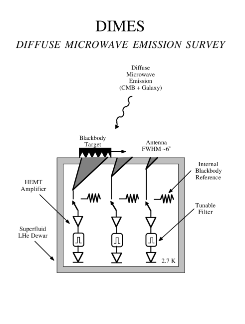
Figure 13.  : Schematic drawing of DIMES instrument.

DIMES uses multiple levels of differences to reduce the effects of offset, drifts, and instrumental signatures. To reduce gain instability or drifts, each receiver is rapidly switched between a cryogenic antenna and a temperature-controlled internal reference load. To eliminate the instrumental signature, each antenna alternately views the sky or a full-aperture target with emissivity $\epsilon>0.9999$. To maximize sensitivity to spectral shape, all frequency channels view the same target in progression, so that deviations from a blackbody spectrum may be determined much more precisely than the absolute blackbody temperature.

DIMES will remove the residual instrument signature by comparing the sky to an external full-aperture blackbody target. The precision achieved will likely be dominated by the thermal stability of the target. While the use of a single external target rejects common-mode uncertainties in the absolute target temperature, thermal gradients within the target or variations of target temperature with time will appear as artifacts in the derived spectra and sky maps. Thermal gradients within the external target are reduced by using a passive multiply-buffered design in which a blackbody absorber (Eccosorb CR-112, an iron-loaded epoxy) is mounted on a series of thermally conductive plates with conductance $G_{1}$ separated by thermal insulators of conductance $G_{2}$. Thermal control is achieved by heating the outermost buffer plate, which is in weak thermal contact with a superfluid helium reservoir. Radial thermal gradients at each stage are reduced by the ratio $G_{2}/G_{1}$ between the buffer plates. Typical materials (Fiberglass and copper) achieve a ratio $G_{2}/G_{1}<10^{-3}$; a two-stage design should achieve net thermal gradients well below 0.1 mK. No heat is applied directly to the absorber, and a conductive copper layer surrounds the absorber on all sides except the front: the Eccosorb lies at the end of an open thermal circuit, eliminating thermal gradients from heat flow.

DIMES will not be limited by raw sensitivity. HEMT amplifiers cooled to 2.7 K easily achieve rms noise 1 mK Hz^-1/2, reaching 0.1 mK sensitivity in 100 seconds of integration. The DIMES spectra are derived from comparison of the sky to the external blackbody target. The largest systematic uncertainties arise from thermal drifts or gradients within the target and emission from warm objects outside the DIMES dewar (e.g., the Earth). Thermometers buried in the microwave absorber monitor thermal gradients and drifts to precision 0.05 mK. Emission from the Earth must be rejected at the -70 dB level to avoid contributing more than 0.1 mK to the total sky signal. DIMES will achieve this rejection using corrugated antennas with 6^∘  beam and good sidelobe response; two sets of shields between the aperture plane and the Earth provide further attenuation of thermal radiation from the Earth. COBE achieved -70 dB attenuation with a 7^∘  beam and a single shield [27], so the DIMES requirement should be attainable.

DIMES will eliminate atmospheric emission completely by observing from low Earth orbit. We are currently investigating the possibility of utilizing the Spartan-400 carrier, which will provide free-flyer capability to Shuttle orbits for 700 kg instruments for a nominal mission of 6 to 9 months.

7 Monopole Spectrum Summary

The previous discussion reviews the observations, results, and future possiblities of the spectrum of the total CMB power. In the next sections we consider the expected signal for a Planckian spectrum for the monopole, dipole and higher order anisotropies and how spectral distortions would appear in the frequency spectrum of various anisotropies.

8 Planckian Radiation Formula

The specific intensity, $I_{\nu}$, of light is defined as the incident energy per unit area, per unit solid angle, per unit frequency.

$$I_{\nu}=\frac{2h\nu^{3}}{c^{2}}n$$ (13)

where $h$ is Planck’s constant, $\nu$ is the frequency, $c$ is the speed of light, and $n$ is the photon occupation number per mode. The intensity or spectral brightness of a blackbody is a function of only one parameter, the temperature

$$B_{\nu}(T)=\frac{2h\nu^{3}}{c^{2}}\frac{1}{e^{x}-1}$$ (14)

where $x=h\nu/kT$. In the Rayleigh-Jeans region $x<<1$ and thus

$$B_{\nu}(T)=\frac{2\nu^{2}}{c^{2}}kT.$$ (15)

The generalization of equation (15) to any $x$ defines the antenna temperature of a blackbody

$$B_{\nu}(T)=\frac{2\nu^{2}}{c^{2}}kT_{ant}(\nu).$$ (16)

Rewriting equation (16) yields the relation between antenna and thermodynamic temperature

$$T_{ant}(\nu)=\frac{h\nu/k}{e^{x}-1}=T\frac{x}{e^{x}-1}.$$ (17)

In the Rayleigh-Jeans portion of a blackbody spectrum the antenna temperature and the thermodynamic temperature are equal ($T_{ant}=T$). Taking the derivative of equation (17) one obtains the relation between antenna and thermodynamic temperature differences

$$\frac{dT_{ant}}{dT}=\frac{x^{2}e^{x}}{(e^{x}-1)^{2}}$$ (18)

where here $x=h\nu/kT_{o}$. The temperature difference conversion depends on a knowledge of $T_{o}$ while equation (16) does not. For example plugging 31.5, 53 and 90 GHz into equation (18) with $T_{o}=2.73$ K, we get the conversion factors 1.026, 1.074, 1.227 respectively.

9 Dipole Formulae

Observers with velocity $\vec{\beta}=\vec{v}/c$ through a Planckian radiation field of temperature $T_{o}$ will measure directionally dependent temperatures,

$$T_{obs}(\theta)=T_{o}\frac{(1-\beta^{2})^{1/2}}{(1-\beta\mu)}$$ (19)

where $\mu=cos\theta$ and $\theta$ is the angle between $\vec{\beta}$ and the direction of observation as measured in the observer’s frame [43].We expand this through order $\beta^{3}$ to show that the dipole is the largest member of a family of kinetic anisotropies,

$$\frac{\Delta T}{T_{o}}=\beta\mu+\frac{\beta^{2}}{2}(2\mu^{2}-1)+\frac{\beta^{3}}{4}(4\mu^{3}-2\mu)+O(\beta^{4}).$$ (20)

or

$$\frac{\Delta T}{T_{o}}=\beta cos\theta+\frac{\beta^{2}}{2}cos2\theta+\frac{\beta^{3}}{4}(4\mu^{3}-2\mu)+O(\beta^{4}).$$ (21)

The antenna temperatures of the CMB, the kinetic dipole and the normalizing quadrupole amplitude are plotted in Figure 12.

In the more general case of non-Planckian spectra $I_{\nu}$ we can define an equivalent antenna temperature by

$$I_{\nu}=\frac{2\nu^{2}}{c^{2}}kT_{ant},$$ (22)

which when combined with equation (18) yields

$$\frac{\Delta I}{I_{o}}=\frac{\Delta T_{ant}}{T_{ant}}=\frac{\Delta T}{T_{o}}\frac{xe^{x}}{(e^{x}-1)},$$ (23)

where $I_{o}$ is an isotropic but not necessarily Planckian radiation field as seen by an observer in the rest frame of the field.

10 The Dipole Anisotropy and Distortions of the CMB Spectrum

The generalization of equation (21) for motion through an isotropic but not necessarily Planckian radiation field of intensity $I_{o}(\nu)$ yields an observed intensity anisotropy,

$$\frac{\Delta I}{I_{o}}(\nu,\theta)=\frac{I_{obs}(\nu,\theta)-I_{o}(\nu)}{I_{o}(\nu)}.$$ (24)

where $\nu$ is the frequency in the observer’s frame and $I_{o}$ is the intensity in the rest frame of the radiation. The result to third order in $\beta$ is [30]

$$\frac{\Delta I}{I_{o}} = \beta\mu(3-\alpha_{1})+\frac{\beta^{2}}{2}\left[2\mu^{2}(6-3\alpha_{1}+\frac{\alpha_{2}}{2})-(3-\alpha_{1})\right]$$ (25)

$$+\frac{\beta^{3}}{4}\left[4\mu^{3}(10-6\alpha_{1}+\frac{3}{2}\alpha_{2}-\frac{1}{6}\alpha_{3})-2\mu(9-5\alpha_{1}+\alpha_{2})\right]+O(\beta^{4})$$

where $\alpha_{n}=\frac{\nu^{n}}{I(\nu)}\frac{\partial^{n}I(\nu)}{\partial\nu^{n}}$. A pedagogical check of this formula can be made by noticing that for a Planckian spectrum $\Delta I/I_{o}=\Delta T_{ant}/T_{ant}=\frac{xe^{x}}{(e^{x}-1)}\Delta T/T_{o}$, where $T_{ant}$ is antenna temperature and $x=h\nu/kT_{o}$. In the Rayleigh-Jeans limit, $\alpha_{1}=\alpha_{2}=2$, $\alpha_{3}=0$ and one obtains $\Delta I/I_{o}=\Delta T/T_{o}$. An analogous simplification does not occur in the Wien limit because of the $\nu$ dependence of the derivatives $\alpha_{n}$. Another check is that an $I\propto\nu^{3}$ non-Planckian spectrum yields no kinetic anisotropy since I/$\nu^{3}$ is a Lorentz invariant. For this case, $\alpha_{1}=3$ and $\alpha_{2}=\alpha_{3}=6$.

Summary The frequency dependence of the dipole anisotropy provides a means to determine the CMB temperature and to detect CMB spectral distortions. In particular accurate measurements of the CMB dipole anisotropy at multiple wavelengths may help in limiting or detecting small spectral distortions. On the other hand accurate spectral measurements are needed for a precise interpretations of the observed anisotropy. It is important to make measurements at as many wavelengths as possible.

10.1 Introduction to Dipole Anisotropy Spectrum

The dipole anisotropy has been measured well at many wavelengths, particularly by the COBE DMR and FIRAS instruments. Prior to that several experiments also measured the dipole anisotropy amplitude and direction.

The most obvious interpretation of the dipole anisotropy is in terms of the peculiar velocity of the solar system; on the other hand it might result from a combination of very long wavelength primordial perturbations [Wilson & Silk 1980)] [58] [42]. We can certainly expect that on the order of 1% of the dipole anisotropy is due to primordial anisotropies based upon a simple extrapolation of the observed anisotropy power spectrum.

Assuming that the observed dipole anisotropy results primarily from the doppler shift due to the peculiar motion of the Solar System, small spectral distortions must give rise via the Compton-Getting effect to a characteristic frequency dependence of the dipole amplitude arising from the shape of the spectral distortions.

10.2 The Compton-Getting Effect

The Compton-Getting effect is, in its original formulation [Compton & Getting 1935], the 24-hour variation in the cosmic ray intensity due to the peculiar velocity of the Earth. This effect is easily generalized as it a straight consequence of the Lorentz invariance of the distribution functions of the particles and photons in phase space (see [Forman 1970)] for a comprehensive discussion).

An observer with velocity v ($\beta$ = v/c) with respect to the reference frame in which the photon distribution function $n(\nu)$ is isotropic to at least first order in $\beta$ will measure a difference between the intensity received in the direction of motion and that received in a direction perpendicular to its motion proportional to:

$$\frac{\Delta n}{n}=\frac{d~{}lnn}{d~{}ln\nu}\beta$$ (26)

Thus measurements of the dipole anisotropy of the CMB intensity yield information on the slope of the spectrum.

To first order in $\beta$ the dipole anisotropy of the CMB intensity is

$$T_{d} = \frac{h\nu}{k}[1/ln(1+1/n(\nu))-1/ln(1+1/n(\nu[1+\beta]))]$$ (27)

$$\approx -\frac{h\nu}{k(1+n)}ln^{-2}(1+\frac{1}{n})\frac{d~{}lnn}{d~{}ln\nu}\beta$$ (28)

In the case of a Planckian spectrum $[n=(exp(x)-1)^{-1};x=h\nu/kT]$ the temperature anisotropy is independent of frequency and

$$\frac{T_{d}}{T}\approx\frac{v}{c}=\beta.$$ (29)

Deviations from a Planckian spectrum, however, lead to a dependence of the dipole anisotropy amplitude, $T_{d}$, specific to the shape of the distortion. Define $\delta$, the first order fractional change in the dipole anisotropy amplitude, to be

$$\delta\equiv\frac{\Delta T_{d}}{T_{do}}\approx[\frac{T_{d}}{T}-\beta]\beta^{-1}.$$ (30)

Now we can calculate and plot the fractional change in dipole amplitude $\delta$ from predicted potential distortions.

10.3 Application to Potential Distortions

The three types of spectral distortions normally discussed are: Comptonization distortion, Bose-Einstein distortion, and free-free distortion. In addition it is sometimes pointed out that there are some very low level distortions expected from the final stages of recombination. Finally, it is possible that there is a generic distortion caused by effects which have not been anticipated, calculated, or otherwise expected. We can make estimates of these also.

Comptonization Distortion

The first order approximation to the photon occupation number for a comptonized spectrum is

$$n_{c}=n_{p}[1+uxexp(x)n_{p}(\frac{x}{tanh(x/2)}-4)]$$ (31)

where the parameter $u=k(T_{e}-T_{\gamma})/m_{e}c^{2}$ is a measure of the amount of extra energy injected into the radiation field. Figure 14 shows the dipole deviation, $\delta$ spectra predicted for such distortions.

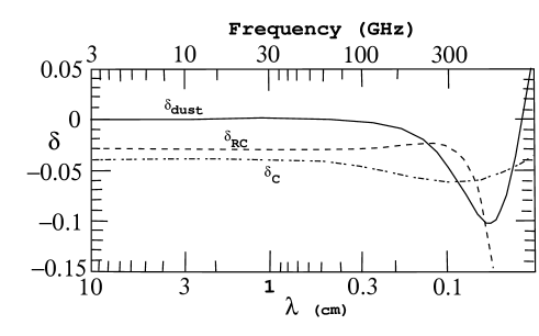
Figure 14.  : Predicted fractional variation of the dipole amplitude ( $\delta=[(T_{d}/T)-\beta]/\beta$ ) for models with non-relativisitc comptonization (C - dot-dashed line), relativisitc comptonization (RC - dashed line), and cold dust (dust - solid line) producing a sub-mm excess.

Bose-Einstein Distortion

In a Bose-Einstein or chemical potential distortion the photon occupation number $n$ is

$$n=\frac{1}{e^{x+\mu_{0}}-1}{\rm~{},}$$ (32)

where $x\equiv{h\nu/kT}$ and $\mu_{0}$ is the dimensionless chemical potential. The chemical potential is predicted to be frequency-dependent,

$$\mu(x)=\mu_{0}e^{-2x_{b}/x}{\rm~{},}$$ (33)

where $x_{b}$ is the transition frequency at which Compton scattering of photons to higher frequencies is balanced by free-free creation of new photons. The resulting spectrum has a sharp drop in brightness temperature at centimeter wavelengths[5] with a minimum at $\lambda_{\rm min}\simeq 4.5~{}\Omega_{B}^{-5/8}~{}{\rm cm}$. Thus the minimum wavelength is determined by $\Omega_{B}$.

We can use this expression for the photon occupation number in the formula for the dipole anisotropy amplitude and find the fractional variation in the dipole anisotropy, $\delta$, for the various possible values of energy release $\mu_{0}\simeq 1.4{\Delta E}/E_{\rm CBR}$ and other cosmological parameters, i.e. $\Omega_{B}$.

To first order the deviation is proportional to $\mu$.

$$\frac{T_{d}}{T}\approx\beta\frac{x^{2}}{(x+\mu)^{2}}(1+\mu\frac{2x_{b}}{x^{2}})$$ (34)

where the second term in the parenthesis is generally small so that so that

$$\delta=-\frac{2\mu x+\mu^{2}}{(x+\mu)^{2}}=-2\mu\frac{x+\mu/2}{(x+\mu)^{2}}$$ (35)

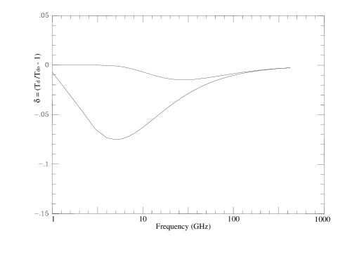
Figure 15.  : Fractional deviation in the dipole anisotropy amplitude due to the doppler shift for two cases of a Bose-Einstein (chemical potential) distortion

Free-Free Distortion

Thermal bremsstrahulung from an ionized intergalactic medium distorts the observed CMB spectrum changing the temperature by an amount

$$\Delta T_{f\!f}=T_{\gamma}\;{Y_{f\!f}}/{x^{2}},$$ (36)

where $T_{\gamma}$ is the undistorted photon temperature, $x$ is the dimensionless frequency, and $Y_{f\!f}/x^{2}$ is the optical depth to free-free emission. The predicted distortion is shown in Figure 16.

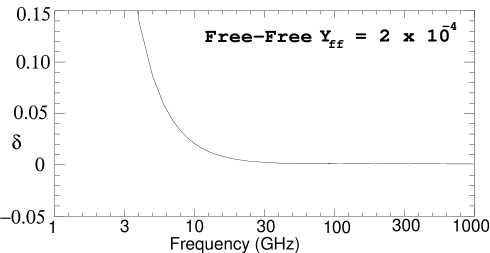
Figure 16.  : Fractional deviation in the dipole anisotropy amplitude from a free-free emission distortion with $Y_{ff}=2\times 10^{-4}$.

Recombination Line Distortion

Since there are on the order of $10^{9}$ CMB photons per baryon, recombination does not have a large effect on the CMB spectrum. However, there are small features ($10^{-4}-10^{-8}$) that result from atomic lines. The best known and calculated are the Lyman-$\alpha$ for hydrogen which appear deep in the Wien region [44]. The result is a step at the high frequency side of the L$\alpha$ resonance (divided by the redshift $z_{\sim}^{<}1100$ of recombination). There is a slight smearing due to the natural line width set by atomic parameters and the thermal motion. The dominant effect is the cosmological expansion redshift which pulls photons from the low frequency side and deposits them on the high frequency side. The final result is a slight step down at the highest frequency at which the resonance was effective.

There are hydrogen resonances at lower frequencies, not only bound-free but also bound-bound transitions, that are manifest in the radio and mm wavelength range. It appears difficult to detect these with an absolute measurement even using a frequency switching system without a very substantial effort. It is likely that using a narrow-bandwidth or spectral receiver observing the dipole anisotropy is a more effective way to observe such a line. The calibration of either such system requires a great deal of care.

Unanticipated Distortions

It is always possible that there are spectral distortions that do not fall in the categories discussed above. In particular, it is quite possible that astrophysical or particle decay/interaction effects could alter the photon occupation number at long wavelengths not yet measured precisely.

Although the precise COBE measurements carry implications for possible distortions at longer wavelengths, the absence of distortions near the peak CMB intensity does not imply correspondingly small distortions at longer wavelengths. Distortions as large as 5% could exist at wavelengths of several centimeters or longer without violating existing observations.

11 SZ Measurements as a Probe of Spectral Distortions

The Sunyaev-Zeldovich [55] effect in the direction of rich clusters of galaxies provides another probe of the CMB spectral shape by means of differential measurements ([19]; [14]; [47]; [60]; [48]). The change in the CMB brightness temperature or intensity is essentially a second order Doppler effect. The amplitude of the effect is proportional to the second derivative of the intensity at the frequency of observation:

$$\frac{\partial I}{\partial y_{C}}=\frac{\partial^{2}I}{\partial(lnx)^{2}}-3\frac{\partial I}{\partial\ln x}{\rm~{},}$$ (37)

where $y_{C}$ is the comptonization parameter of the cluster and $x=h\nu/kT_{0}$. If the intensity ($I\propto x^{\alpha}$) is locally a power law with exponent $\alpha$, then $\partial I/\partial y_{C}\propto\alpha(\alpha-3)$. In the Rayleigh-Jeans region, $\alpha=2$; it then decreases with increasing frequency and becomes negative in the Wein region. The Sunyaev-Zeldovich effect changes signs around the CMB spectrum peak. The spectrum of the SZ effect is sensitive to the detailed shape of the original CMB spectrum. Figure 17 shows examples of the predicted effect.

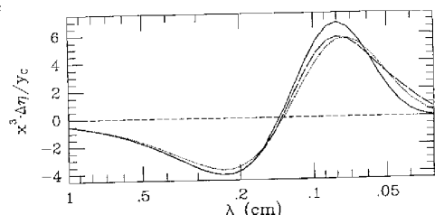
Figure 17.  : The predicted Sunyaev-Zeldovich effect corresponding to a Planck spectrum (solid line) and two spectral distortions: non-relativisitc comptonization (dotted line) and a cold dust emission (long dashes) creating a sub-mm excess. For the ordinate $x=h\nu/kT;x^{3}\Delta n$ is a quantity proportional to the change of the CMB intensity, $y_{C}$ is the comptonization parameter for the cluster.

Two things, in addition to observational noise and errors, act to confuse. The first confusion is that the shape of the SZ effect is slightly modified by the temperature distribution of the hot electrons in the galactic cluster ([48]). The second confusion is any local cluster or foreground emission contributions to the observed intensity. Fortunately, foreground emissions will not have a dipole pattern or SZ effect and measurements of this kind can be used to separate out extragalactic contributions to the observed flux.

12 CMB Anisotropy Frequency Spectrum

Given the precise observations of the monopole and dipole frequency spectrum, then we can confidently predict the frequency spectrum of higher order CMB anisotropies. The frequency spectrum should be the same as that for the dipole anisotropy (except for the special case of the thermal SZ effect). This is a fundamental assumption underlying techniques for separating the observations of the microwave sky into its CMB and foreground components.

We can ask, based on the COBE data, how well is this assumption verified. It turns out tha FIRAS alone does not have sufficient resolution to measure the higher order anisotropy frequency spectrum. That is FIRAS can readily measure the dipole frequency spectrum but is not able to measure that of the quadrupole, octopole, etc. on its own. However, if the FIRAS observations are crosscorrelated with the DMR observations, then one can make an estimate of the anisotropy frequency spectrum [17]. This technique can and has been used with external experiments such as FIRS, Tenerife, Saskatoon and will be with future observations; but these other observations are currently much more limited than FIRAS in frequency samplingng.

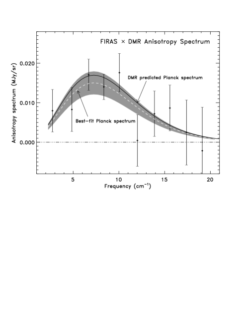
Figure 18.  : The frequency spectrum of primordial CMB distortions determined by crosscorrelation of the COBE DMR and FIRAS data sets. The points with errors are the results of correlating the DMR CMB anisotropy map with the FIRAS map generated by removing the monopole, dipole, and an estimate of the Galactic dust emission. The thin line is the predicted spectrum based upon the DMR data alone and the assumption of a precisely Planckian CMB spectrum. The band with centered line is the best-fitted Planckian CMB spectrum to the FIRAS-DMR crosscorrelation.

The observations of the CMB thermal spectrum and the frequency spectra of anisotropies are point to a precisely thermal spectrum for the CMB. This figure [17] shows the three levels of frequency spectra: monopole, dipole, higher order anisotropies left after Galactic dust emission is removed.

Figure 19.  : Frequency Spectrum of CMB features: (a) The CMB monopole frequency spectrum as measured by FIRAS and a line for a Planckian. (b) The CMB dipole frequency spectrum as measured by FIRAS and a line indicating the anisotropy frequency spectrum expected for a Planckian. (c) The frequency spectrum of Galactic dust emission removed from the FIRAS spectrum. (d) The CMB higher order anisotropy frequency spectrum as measured by FIRAS and a line indicating the anisotropy frequency spectrum expected for a Planckian.

13 Acknowledgments

This work was supported in part by the Director, Office of Energy Research, Office of High Energy and Nuclear Physics, Division of High Energy Physics of he U.S. Department of Energy under contract No. DE-AC03-76SF00098.

TABLE 4.  : Measurements of $T_{CMB}$

 Frequency Wavelength Temperature Location Reference (GHz) (cm) (K) (calibration)  0.408 73.5 $3.7\pm 1.2$ Ground (LN) Howell & Shakeshaft 1967, Nature, 216, 753. 0.6 50 $3.0\pm 1.2$ Ground (Term) Sironi et al. 1990, Ap.J., 357, 301. 0.610 49.1 $3.7\pm 1.2$ Ground (LN) Howell & Shakeshaft 1967, Nature, 216, 7 0.635 47.2 $3.0\pm 0.5$ Ground (LN) Stankevich et al 1970, Australian J. Phys, 23, 529 0.820 36.6 $2.7\pm 1.6$ Ground (Term) Sironi et al. 1991, Ap.J., 378, 550. 1 30 $2.5\pm 0.3$ Ground (LN) Pelyushenko & Stankevich 1969, Sov. Astron., 13, 223. 1.4 21.3 $2.11\pm 0.38$ Ground (CLC) Levin et al. 1988, Ap.J., 334,14 1.42 21.2 $3.2\pm 1.0$ Ground (Term) Penzias and Wilson 1967, AJ, 72, 315 1.43 21 $2.65^{+0.33}_{-0.30}$ Ground (LN) Staggs et al. 1996, ApJ, 458, 407 1.44 20.9 $2.5\pm 0.3$ Ground (LN) Pelyushenko & Stankevich 1969, Sov. Astron., 13, 223. 1.45 20.7 $2.8\pm 0.6$ Ground (Term) Howell & Shakeshaft 1966, Nature, 210, 1318. 1.47 20.4 $2.27\pm 0.19$ Ground (CLC) Bensadoun et al. 1992 (in press) 2 15 $2.5\pm 0.3$ Ground (LN) Pelyushenko & Stankevich 1969, Sov. Astron., 13, 223. 2.3 13.1 $2.66\pm 0.77$ Ground (Term) Otoshi & Stelzreid 1975, IEEE Trans on Inst & Meas, 24, 174. 2.5 12 $2.71\pm 0.21$ Ground (CLC) Sironi et al. 1991, Ap. J., 378, 550. 3.8 7.9 $2.64\pm 0.06$ Ground (CLC) De Amici et al. 1991, Ap.J., 381, 341. 4.08 7.35 $3.5\pm 1.0$ Ground (Term) Penzias & Wilson 1965, Ap.J., 142, 419. 4.75 6.3 $2.70\pm 0.07$ Ground (CLC) Mandolesi et al. 1986, Ap.J., 310, 561. 7.5 4.0 $2.60\pm 0.07$ Ground (CLC) Kogut et al. 1988, Ap.J., 355, 102 7.5 4.0 $2.64\pm 0.06$ Ground (CLC) Levin et al. 1992, Ap.J., 396, 3 9.4 3.2 $3.0\pm 0.5$ Ground (Term) Roll & Wilkinson 1966, Phys. Rev. Lett., 16, 405. 9.4 3.2 $2.69^{+0.16}_{-0.21}$ Ground (CLC) Stokes et al. 1967, Phys. Rev. Lett., 19, 1199. 10 3.0 $2.62\pm 0.06$ Ground (CLC) Kogut et al. 1990, Ap.J., 355, 102. 10.7 2.8 $2.730\pm 0.014$ Balloon (LHe) Staggs et al. 1996, ApJ, 458, 407 19.0 1.58 $2.78^{+0.12}_{-0.17}$ Ground (CLC) Stokes et al. 1967, Phys. Rev. Lett., 19, 1199. 20 1.5 $2.0\pm 0.4$ Ground (CLC) Welch et al. 1967, Phys. Rev. Lett, 18, 1068. 24.8 1.2 $2.783\pm 0.025$ Balloon Johnson & Wilkinson 1987, Ap.J. Lett, 313, L1. 32.5 0.924 $3.16\pm 0.26$ Ground (CLC) Ewing et al. 1967, Phys. Rev. Lett, 19, 1251. 33.0 0.909 $2.81\pm 0.12$ Ground (CLC) De Amici et al. 1985, Ap.J., 298, 710. 35.0 0.856 $2.56^{+0.17}_{-0.22}$ Ground (CLC) Wilkinson 1967, Phys. Rev. Lett., 19, 1195. 37 0.82 $2.9\pm 0.7$ Ground (LN) Puzanov et al. 1968, Sov. Astr., 11, 905. 83.8 0.358 $2.4\pm 0.7$ Ground (LN) Kislyakov et al. 1971, Sov. Ast., 15, 29. 90 0.33 $2.46^{+0.40}_{-0.44}$ Ground (CLC) Boynton et al. 1968, Phys. Rev. Lett., 21, 462. 90 0.33 $2.61\pm 0.25$ Ground (CLC) Millea et al. 1971, Phys. Rev. Lett., 26, 919. 90 0.33 $2.48\pm 0.54$ Plane (Term) Boynton & Stokes 1974, Nature, 247, 528. 90 0.33 $2.60\pm 0.09$ Ground (CLC) Bersanelli et al. 1989, Ap.J., 339, 632. 90.3 0.332 $2.97\pm 1.0$ Balloon Bernstein et al. 1990, Ap.J., 362, 107. 113.6 0.264 $2.70\pm 0.04$ CN (z Per) Meyer & Jura 1985, Ap.J., 297, 119. 113.6 0.264 $2.74\pm 0.05$ CN (z Oph) Crane et al. 1986, Ap.J., 309, 12. 113.6 0.264 $2.76\pm 0.07$ CN (HD 21483) Meyer et al. 1989, Ap.J. Lett, 343, L1. 113.6 0.264 $2.796^{+0.014}_{-0.039}$ CN (z Oph) Crane et al. 1989, Ap.J., 346, 136. 113.6 0.264 $2.75\pm 0.04$ CN (z Per) Kaiser & Wright 1990, Ap.J. Lett, 356, L1. 113.6 0.264 $2.834\pm 0.085$ CN (HD 154368) Palazzi et al. 1990, Ap.J., 357, 14. 113.6 0.264 $2.807\pm 0.025$ CN (16 stars) Palazzi et al. 1992, Ap.J., 398, 53. 154.8 0.194 $3.02\pm 1.0$ Balloon Bernstein et al. 1990, Ap.J., 362, 107. 195.0 0.154 $2.91\pm 1.0$ Balloon Bernstein et al. 1990, Ap.J., 362, 107. 227.3 0.132 $2.76\pm 0.20$ CN (z Per) Meyer & Jura 1985, Ap.J., 297, 119. 227.3 0.132 $2.75^{+0.24}_{-0.29}$ CN (z Oph) Crane et al. 1986, Ap.J., 309, 822. 227.3 0.132 $2.83\pm 0.09$ CN (HD 21483) Meyer et al. 1989, Ap.J. Lett, 343, L1. 227.3 0.132 $2.832\pm 0.072$ CN (HD 154368) Palazzi et al. 1990, Ap.J., 357, 14. 266.4 0.113 $2.88\pm 1.0$ Balloon Bernstein et al. 1990, Ap.J., 362, 107.  

TABLE 5.  : Measurements of $T_{CMB}$

Frequency Wavelength Temperature Location Reference (GHz) (cm) (K) (calibration) 0.408 73.5 $3.7\pm 1.2$ Ground (LN) Howell & Shakeshaft 1967, Nature, 216, 753. 0.6 50 $3.0\pm 1.2$ Ground (Term) Sironi et al. 1990, Ap.J., 357, 301. 0.610 49.1 $3.7\pm 1.2$ Ground (LN) Howell & Shakeshaft 1967, Nature, 216, 7 0.635 47.2 $3.0\pm 0.5$ Ground (LN) Stankevich et al 1970, Australian J. Phys, 23, 529 0.820 36.6 $2.7\pm 1.6$ Ground (Term) Sironi et al. 1991, Ap.J., 378, 550. 1 30 $2.5\pm 0.3$ Ground (LN) Pelyushenko & Stankevich 1969, Sov. Astron., 13, 223. 1.4 21.3 $2.11\pm 0.38$ Ground (CLC) Levin et al. 1988, Ap.J., 334,14 1.42 21.2 $3.2\pm 1.0$ Ground (Term) Penzias and Wilson 1967, AJ, 72, 315 1.43 21 $2.65^{+0.33}_{-0.30}$ Ground (LN) Staggs et al. 1996, ApJ, 458, 407 1.44 20.9 $2.5\pm 0.3$ Ground (LN) Pelyushenko & Stankevich 1969, Sov. Astron., 13, 223. 1.45 20.7 $2.8\pm 0.6$ Ground (Term) Howell & Shakeshaft 1966, Nature, 210, 1318. 1.47 20.4 $2.27\pm 0.19$ Ground (CLC) Bensadoun et al. 1992 (in press) 2 15 $2.5\pm 0.3$ Ground (LN) Pelyushenko & Stankevich 1969, Sov. Astron., 13, 223. 2.3 13.1 $2.66\pm 0.77$ Ground (Term) Otoshi & Stelzreid 1975, IEEE Trans on Inst & Meas, 24, 174. 2.5 12 $2.71\pm 0.21$ Ground (CLC) Sironi et al. 1991, Ap. J., 378, 550. 3.8 7.9 $2.64\pm 0.06$ Ground (CLC) De Amici et al. 1991, Ap.J., 381, 341. 4.08 7.35 $3.5\pm 1.0$ Ground (Term) Penzias & Wilson 1965, Ap.J., 142, 419. 4.75 6.3 $2.70\pm 0.07$ Ground (CLC) Mandolesi et al. 1986, Ap.J., 310, 561. 7.5 4.0 $2.60\pm 0.07$ Ground (CLC) Kogut et al. 1988, Ap.J., 355, 102 7.5 4.0 $2.64\pm 0.06$ Ground (CLC) Levin et al. 1992, Ap.J., 396, 3 9.4 3.2 $3.0\pm 0.5$ Ground (Term) Roll & Wilkinson 1966, Phys. Rev. Lett., 16, 405. 9.4 3.2 $2.69^{+0.16}_{-0.21}$ Ground (CLC) Stokes et al. 1967, Phys. Rev. Lett., 19, 1199. 10 3.0 $2.62\pm 0.06$ Ground (CLC) Kogut et al. 1990, Ap.J., 355, 102. 10.7 2.8 $2.730\pm 0.014$ Balloon (LHe) Staggs et al. 1996, ApJ, 458, 407 19.0 1.58 $2.78^{+0.12}_{-0.17}$ Ground (CLC) Stokes et al. 1967, Phys. Rev. Lett., 19, 1199. 20 1.5 $2.0\pm 0.4$ Ground (CLC) Welch et al. 1967, Phys. Rev. Lett, 18, 1068. 24.8 1.2 $2.783\pm 0.025$ Balloon Johnson & Wilkinson 1987, Ap.J. Lett, 313, L1.

TABLE 6.  : Measurements of $T_{CMB}$ Continued

Frequency Wavelength Temperature Location Reference (GHz) (cm) (K) (calibration) 32.5 0.924 $3.16\pm 0.26$ Ground (CLC) Ewing et al. 1967, Phys. Rev. Lett, 19, 1251. 33.0 0.909 $2.81\pm 0.12$ Ground (CLC) De Amici et al. 1985, Ap.J., 298, 710. 35.0 0.856 $2.56^{+0.17}_{-0.22}$ Ground (CLC) Wilkinson 1967, Phys. Rev. Lett., 19, 1195. 37 0.82 $2.9\pm 0.7$ Ground (LN) Puzanov et al. 1968, Sov. Astr., 11, 905. 83.8 0.358 $2.4\pm 0.7$ Ground (LN) Kislyakov et al. 1971, Sov. Ast., 15, 29. 90 0.33 $2.46^{+0.40}_{-0.44}$ Ground (CLC) Boynton et al. 1968, Phys. Rev. Lett., 21, 462. 90 0.33 $2.61\pm 0.25$ Ground (CLC) Millea et al. 1971, Phys. Rev. Lett., 26, 919. 90 0.33 $2.48\pm 0.54$ Plane (Term) Boynton & Stokes 1974, Nature, 247, 528. 90 0.33 $2.60\pm 0.09$ Ground (CLC) Bersanelli et al. 1989, Ap.J., 339, 632. 90.3 0.332 $2.97\pm 1.0$ Balloon Bernstein et al. 1990, Ap.J., 362, 107. 113.6 0.264 $2.70\pm 0.04$ CN (z Per) Meyer & Jura 1985, Ap.J., 297, 119. 113.6 0.264 $2.74\pm 0.05$ CN (z Oph) Crane et al. 1986, Ap.J., 309, 12. 113.6 0.264 $2.76\pm 0.07$ CN (HD 21483) Meyer et al. 1989, Ap.J. Lett, 343, L1. 113.6 0.264 $2.796^{+0.014}_{-0.039}$ CN (z Oph) Crane et al. 1989, Ap.J., 346, 136. 113.6 0.264 $2.75\pm 0.04$ CN (z Per) Kaiser & Wright 1990, Ap.J. Lett, 356, L1. 113.6 0.264 $2.834\pm 0.085$ CN (HD 154368) Palazzi et al. 1990, Ap.J., 357, 14. 113.6 0.264 $2.807\pm 0.025$ CN (16 stars) Palazzi et al. 1992, Ap.J., 398, 53. 154.8 0.194 $3.02\pm 1.0$ Balloon Bernstein et al. 1990, Ap.J., 362, 107. 195.0 0.154 $2.91\pm 1.0$ Balloon Bernstein et al. 1990, Ap.J., 362, 107. 227.3 0.132 $2.76\pm 0.20$ CN (z Per) Meyer & Jura 1985, Ap.J., 297, 119. 227.3 0.132 $2.75^{+0.24}_{-0.29}$ CN (z Oph) Crane et al. 1986, Ap.J., 309, 822. 227.3 0.132 $2.83\pm 0.09$ CN (HD 21483) Meyer et al. 1989, Ap.J. Lett, 343, L1. 227.3 0.132 $2.832\pm 0.072$ CN (HD 154368) Palazzi et al. 1990, Ap.J., 357, 14. 266.4 0.113 $2.88\pm 1.0$ Balloon Bernstein et al. 1990, Ap.J., 362, 107.

TABLE 7.  : FIRAS Data; [16]

TABLE 8.  : FIRAS Data – continued; [16]

TABLE 9.  : FIRAS Data; [16]

TABLE 10.  : FIRAS Data – continued; [16]

TABLE 11.  : UBC COBRA Rocket Data; [21]

TABLE 12.  : UBC COBRA Rocket Data – continued; [21]

TABLE 13.  : UBC COBRA Rocket Data; [21]

TABLE 14.  : UBC COBRA Rocket Data – continued; [21]

References

- [1] W.S. Adams Ap. J.93, 11 (1941)
- [2] R.A. Alpher and R.C. Herman, Physics Today, Vol. 41, No. 8, p. 24 (1988)
- [3] J.G. Bartlett and A. Stebbins, Ap. J.371,8(1991)
- [4] M. Bersanelli et al., Ap. J.424, 517 (1994)
- [5] C. Burigana, L. Danese, and G.F. De Zotti, Astronmy & Astrophysics246, 49 (1991)
- [6] M.T. Ceballos and X. Barcons, MNRAS 271, 817 (1994)
- [Compton & Getting 1935] Compton, A.H., Getting, I.A., 1935, Phys. Rev., 47, 817
- [7] P. Crane, D.J. Hegyi, N. Mandolesi, & A.C. Danks Ap. J., 309, 822 (1986)
- [8] P. Crane, D.J. Hegyi, M.L. Kutner, & N. Mandolesi Ap. J., 346, 136 (1989)
- [Danese & De Zotti (1981)] Danese, L. & De Zotti, G. 1981, Astron. Astrophysics, 84, 364
- [9] L. Danese and G.F. De Zotti, Astronmy & Astrophysics107, 39 (1982)
- [10] R. Daly, Ap. J.371, 14 (1992)
- [11] G. De Zotti, ppnp17, 117 (1987)
- [12] R.H. Dicke, P.J.E. Peebles, P.G. Roll, and D.T. Wilkinson, Ap. J.142, 414 (1965)
- [13] John Ellis, G.B. Gelmini, Jorge L. Lopez, D.V. Nanopoulos, Subir Sarkar, Nucl. Phys. B373 (1992) 399-437.
- [14] R. Fabbri, F. Melchiorri, & V. Natale 1978 Astropysics & Space Science 59, 223
- [15] R. Fabbri 1981 Astropysics & Space Science 77, 529
- [16] D.J. Fixsen et al., Astrophys. J., in press (1996)
- [17] Fixsen D.J., Hinshaw, G., Bennett, C.L., & Mather, J.C., ApJ, in press (1997), astro-ph/9704176.
- [Forman 1970)] Forman, M.A. 1970, Planet. Space Sci. 18, 25
- [18] Ge et al. 1997 ApJ, 474, 67
- [19] R.J. Gould & Y. Rephaeli 1978 Ap. J.219, 12
- [20] Górski K.M., Banday, A.J., Bennett, C.L., Hinshaw, G., Kogut, A., Smoot, G.F., & Wright, E.L., 1996, ApJ, 464, in press
- [21] Gush et al. 1990, Phys. Rev. Lett, 65, 537.
- [22] W. Hu and J. Silk, Phy. Rev.170, 2661 (1993)
- [23] W. Hu, D. Scott, & J. Silk, Ap. J.430, L5 (1994)
- [24] B.J.T. Jones & G. Steigman Mon. Not. R. Astr. Soc. 183, 585 (1978)
- [25] A. Kogut, S.J. Petuchowski, C.L. Bennett, & G.F. Smoot, Ap. J., 348, L45 (1990)
- [26] A. Kogut et al., Ap. J.419, 1 (1993)
- [27] A. Kogut et al., Ap. J.470, 1? (1996)
- [28] A. Kogut Moriond CMB Conference Proceedings (1996)
- [29] J.J. Levin, K. Freese & D.N. Spergel, Ap. J.389, 464 (1992)
- [30] C. Lineweaver, G. F. Smoot, L. Tenorio, & A. Kogut (1995), Astrophysical Letters & Communications 32, 173.
- [31] C. Lineweaver et al., (1996) Astrophys. J., 470, 38 (astro-ph/9601151)
- [32] Liddle, A.R. & Lyth, D.H. 1995, MNRAS, 273, 1177
- [33] J.C. Mather et al., Ap. J.420, 439 (1994)
- [34] A. Mckellar, Publ. Dominion Astrophys. Observatory, 1, 251 (1941)
- [35] D.M. Meyer & M. Jura Ap. J., 297, 119 (1985)
- [36] D.M. Meyer, K.C. Roth, & I. Hawkins Ap. J., 343, L1 (1989)
- [37] J.V. Narlikar & N.C. Rana Phys. Lett. 77A, 219 (1980)
- [38] P.D. Noerdlinger Phy. Rev. Let. 30, 761 (1973)
- [39] J.P. Ostriker & C. Thompson Ap. J.323, L97 (1987)
- [40] E. Palazzi et al. Ap. J.357, 14 (1990)
- [41] E. Palazzi, N. Mandolesi, & P. Crane Ap. J.398, 53 (1992)
- [42] Paczynski & Piran 1990
- [43] P.J.E. Peebles & D.T. Wilkinson 1968 PR 174, 2168
- [44] P.J.E. Peebles, “Principles of Physical Cosmology,” Princeton U. Press, p. 168 (1993)
- [45] A.A. Penzias and R. Wilson, Ap. J.142, 419 (1965)
- [46] M. D. Pollock Mon. Not. R. Astr. Soc. 193, 825-831 (1973)
- [47] Y. Rephaeli, Ap. J., 241, 858
- [48] Y. Rephaeli, Ann. Rev. Astron. & Astrophysics, 33:541-579
- [49] K.C. Roth, D.M. Meyer, & I. Hawkins Ap. J., 420, L67-71 (1993)
- [50] K.C. Roth & D.M. Meyer Ap. J., 441, 129 (1995)
- [51] A. Songaila et al. Nature 368, 599 (1994)
- [52] A. Songaila et al. Nature 371, 43 (1994)
- [Smoot et al. 1977)] Smoot, G.F., Gorenstein, M.V., Muller, R.A. 1977, Phys. Rev. Let., 39, 898
- [53] Sarkar, S., & Cooper, A.M., Phys. Lett. 148B (1984) 347-354.
- [54] R.A. Sunyaev and Ya.B. Zel’dovich, Ann. Rev. Astron. & Astrophysics18, 537 (1980)
- [55] R.A. Sunyaev and Ya.B. Zel’dovich, Comm. Astrophys. Space Physics. 4, 173 (1972)
- [56] Tegmark, M., Silk, J., & Blanchard, A., 1994, ApJ, 420, 484
- [57] P. Thaddeus Ann. Rev. Astron. & Astrophy. 10, 305 (1972)
- [58] M. Turner 1991 Phys. Rev. D. 44, 3737.
- [Wilson & Silk 1980)] Wilson, M.L. & Silk, J. 1980, Ap.J.
- [59] E.L. Wright, Ap. J.232, 348 (1979)
- [60] E.L. Wright, Ap. J.232, 348 (1979)
- [61] E.L. Wright et al., Ap. J.420, 450 (1994) CMB Spectrum References LBL-Italy: G. F. Smoot et al., Phy. Rev. Let.51,1099(1983) M. Bensadoun et al., Ap. J., 409, 1.(1993) M. Bersanelli et al., Ap. J., (1994) M. Bersanelli et al., Astro Lett and Communications 32, 7-13 (1996) De Amici, G. et al., Ap. J., 381, 341 (1991) N. Mandolesi et al., Ap. J., 310, 561 (1986) G. Sironi, G. Bonelli, and M. Limon, Ap. J., 378, 550 (1991) FIRAS: J. C. Mather et al., Ap. J.432,L15(1993) D. Fixsen et al., Ap. J., 420, 445 (1994) D. Fixsen et al., Ap. J., in press (1996) DMR: Kogut et al., Ap. J.419,1 (1993) A. Kogut et al., Ap. J., submitted (1996) Princeton: Staggs, S. et al.Astrophys. Lett & Comm, 32, 99 (1995) D. G. Johnson and D. T. Wilkinson , Ap. J.,313, L1 (1987) UBC: H. P. Gush, M. Halperin, and E. H. Wishnow Phy. Rev. Let.,65, 537 (1990) Cyanogen: D. M. Meyer et al., Ap. J., 297, 119 (1985) E. Palazzi, et al., Ap. J., 357, 14 (1990) Staggs Staggs et al. 1996, ApJ, 473, L1 Staggs et al. 1996, ApJ, 458, 407