Improved evidence for a black hole in M32 from HST/FOS spectra —
II. Axisymmetric dynamical models

Abstract

Axisymmetric dynamical models are constructed for the E3 galaxy M32 to interpret high spatial resolution stellar kinematical data obtained with the Hubble Space Telescope (HST). Models are studied with two-integral, $f(E,L_{z})$, phase-space distribution functions, and with fully general three-integral distribution functions. The latter are built using an extension of Schwarzschild’s approach: individual orbits in the axisymmetric potential are calculated numerically, and populated using non-negative least-squares fitting so as to reproduce all available kinematical data, including line-of-sight velocity profile shapes. The details of this method are described in companion papers by Rix et al. and Cretton et al.

Models are constructed for inclinations $i=90^{\circ}$ (edge-on) and $i=55^{\circ}$. No model without a nuclear dark object can fit the combined ground-based and HST data, independent of the dynamical structure of M32. Models with a nuclear dark object of mass $M_{\bullet}=3.4\times 10^{6}\>{\rm M_{\odot}}$ (with $1\sigma$ and $3\sigma$ error bars of $0.7\times 10^{6}\>{\rm M_{\odot}}$ and $1.6\times 10^{6}\>{\rm M_{\odot}}$, respectively) do provide an excellent fit. The inclined models provide the best fit, but the inferred $M_{\bullet}$ does not depend sensitively on the assumed inclination. The models that best fit the data are not two-integral models, but like two-integral models they are azimuthally anisotropic. Two-integral models therefore provide useful low-order approximations to the dynamical structure of M32. We use them to show that an extended dark object can fit the data only if its half-mass radius is $r_{\rm h}\lesssim 0.08^{\prime\prime}$ ($=0.26\>{\rm pc}$), implying a central dark matter density exceeding $1\times 10^{8}\>{\rm M_{\odot}}\>{\rm pc}^{-3}$.

The inferred $M_{\bullet}$ is consistent with that suggested previously by ground-based kinematical data. However, radially anisotropic axisymmetric constant mass-to-light ratio models are now ruled out for the first time, and the limit on the dark matter density implied by the HST data is now stringent enough to rule out most plausible alternatives to a massive black hole. Thus, the evidence for a massive black hole in the quiescent galaxy M32 is now very compelling.

The dynamically inferred $M_{\bullet}$ is identical to that suggested by existing models for HST photometry of M32 that assume adiabatic growth (over a time scale exceeding $10^{6}\>{\rm yr}$) of a black hole into a pre-existing core. The low activity of the nucleus of M32 implies either that only a very small fraction of the gas that is shed by evolving stars is accreted onto the black hole, or alternatively, that accretion proceeds at very low efficiency, e.g. in an advection-dominated mode.

1 Introduction

It is generally believed that active galaxies and quasars are powered by the presence of massive black holes (BHs) in their nuclei, and that such BHs are present in many, possibly all, quiescent galaxies as well (see Kormendy & Richstone 1995, Lynden-Bell 1996 and Rees 1996 for reviews of this paradigm and its history). Evidence for this can be derived from studies of the dynamics of stars and gas in the nuclei of individual galaxies. The high spatial resolution data that can now be obtained with the Hubble Space Telescope (HST) allows the existing evidence to be strengthened considerably. The present paper is part of a new HST study of the quiescent galaxy M32, in which the presence of a BH has long been suspected based on the steep central rotation velocity gradient and nuclear peak in the velocity dispersion seen in ground-based data (e.g., Tonry 1987; van der Marel et al. 1994a; Bender, Kormendy & Dehnen 1996). The main results of our project were summarized, and discussed in the context of other recent work, in van der Marel et al. (1997a). The acquisition and reduction of the stellar kinematical HST data were described in van der Marel, de Zeeuw & Rix (1997b; hereafter Paper I). Here we present new dynamical models that we have used to interpret the combined HST and ground-based data.

Two types of self-consistent dynamical models have been constructed previously to interpret the ground-based data for M32. Dressler & Richstone (1988) and Richstone, Bower & Dressler (1990) used a method based on Schwarzschild’s (1979) technique, in which individual orbits are calculated and superposed, to provide a self-consistent model that fits a given set of data. These ‘maximum entropy’ (Richstone & Tremaine 1988) models could fit the (then available) data only by invoking the presence of a central dark mass of $(0.7$–$8)\times 10^{6}M_{\odot}$. The models are general in the sense that they make no assumptions about the dynamical structure of the galaxy. However, a drawback was that only spherical geometry was considered. Even though the models can be made to rotate, it remains unclear what systematic errors are introduced when they are applied to a flattened (E3) galaxy like M32. An alternative approach has been to construct axisymmetric models with phase-space distribution functions (DFs) that depend only on the two classical integrals of motion, $f=f(E,L_{z})$, where $E$ is the binding energy and $L_{z}$ is the angular momentum component along the symmetry axis, both per unit mass. These models properly take flattening and rotation into account. To fit the M32 data, they require the presence of a central dark mass between $1.8\times 10^{6}M_{\odot}$ (van der Marel et al. 1994b; Qian et al. 1995; Dehnen 1995) and $3\times 10^{6}M_{\odot}$ (Bender, Kormendy & Dehnen 1996). The disadvantage of these models is that they have a special dynamical structure. The velocity dispersions in the meridional plane are isotropic, $\sigma_{r}=\sigma_{\theta}$, which might not be the case in M32. However, the models do fit the observed line-of-sight velocity profile (VP) shapes without invoking freely adjustable parameters, which provides some reason to believe that the M32 DF may not be too different from the form $f(E,L_{z})$.

The previous work on M32 has shown that models with a BH can fit the ground-based data, but the modeling has not been general enough to demonstrate that a BH is required. In fact, the spatial resolution of the ground-based data might have been insufficient for this to be the case (see Appendix A for a discussion of this issue). It has certainly not been sufficient to rule out a cluster of dark objects (as opposed to a central BH) on the basis of theoretical arguments; Goodman & Lee (1989) showed that this requires a resolution of $\lesssim 0.1^{\prime\prime}$. Our new HST data of the nuclear region of M32 were obtained with the HST Faint Object Spectrograph (FOS) through square apertures of $0.068^{\prime\prime}$ and $0.191^{\prime\prime}$, respectively, yielding the highest spatial resolution stellar kinematical data for M32 obtained to date. The results (see, e.g., Figure 2 below) show a steeper rotation curve and higher central velocity dispersion than the best ground-based M32 data. The primary goals of our project are to determine whether these new HST data rigorously rule out models without any dark mass, and to what extent they constrain the mass and size of the dark object in M32.

To obtain constraints on the presence of a dark object that are least dependent on a priori assumptions about the DF, we need to compare the HST data not only to the predictions of axisymmetric $f(E,L_{z})$ models, but also to the predictions of models with a fully general dynamical structure. Orbit superposition techniques provide the most straightforward approach to construct such models. However, orbit superposition is more difficult to implement for the axisymmetric case than for the spherical case: the orbits are not planar and typically possess an additional integral of motion, so that the orbit library must sample three rather than two integrals of motion. Furthermore, a larger parameter space must be explored because of the unknown inclination angle. This implies that larger amounts of CPU time and computer memory are required. However, other than that, there are no reasons why such models would be infeasible. Motivated by the increased speed and memory capacity of computers, we therefore developed a technique to construct fully general axisymmetric orbit superposition models, that fit any given number of observed photometric and kinematic constraints. Independent software implementations were written by H.-W.R, N.C. and R.v.d.M. Our technique may be viewed as the axisymmetric generalization of the spherical modeling used by Richstone and collaborators, with the important additional feature that we calculate VP shapes and include an arbitrary number of Gauss-Hermite moments in the fit. We take into account the error on each observational constraint to obtain an objective $\chi^{2}$ measure for the quality-of-fit. Our basic algorithm is described in Rix et al. (1997; hereafter R97) and summarized in de Zeeuw (1997). R97 provide an application to the spherical geometry; Cretton et al. (1997; hereafter C97) present the extension to the axisymmetric case. Here we summarize the main steps of the axisymmetric algorithm briefly, and focus on the application to M32. The resulting models are the most general yet constructed for M32.

The paper is organized as follows. In Section 2 we discuss our parametrizations for the stellar mass density and for the potential of the dark object. In Section 3 we describe the construction of models with $f(E,L_{z})$ DFs, and in Section 4 we compare the predictions of these models, both with and without BHs, to the kinematical data. In Section 5 we outline the orbit-superposition technique for constructing models with a fully general dynamical structure, and in Section 6 we compare the predictions of these models to the data. We construct models with an extended dark object in Section 7. We summarize and discuss our main conclusions in Section 8. Readers interested primarily in the results of our models may wish to skip Sections 2, 3 and 5.

2 Mass density and potential

We adopt a parametrized form for the axisymmetric mass density of M32:

$$\rho(R,z)=\rho_{0}\>(m/b)^{\alpha}\>[1+(m/b)^{2}]^{\beta}\>[1+(m/c)^{2}]^{\gamma},\qquad m^{2}\equiv R^{2}+(z/q)^{2}.$$ (1)

The mass density $\rho$ is related to the luminosity density $j$ according to $\rho=\Upsilon j$, where $\Upsilon$ is the average mass-to-light ratio of the stellar population (hereafter given in solar V-band units). Both $\Upsilon$ and the intrinsic axial ratio $q$ are assumed to be constant (as a function of radius). The projected axial ratio $q_{p}$ is determined by the inclination $i$ according to $q_{p}^{2}=\cos^{2}i+q^{2}\sin^{2}i$. The parameters $\Upsilon$ and $i$ can be freely specified; all other parameters are determined by fitting to the available M32 surface photometry.

The highest spatial resolution surface photometry available for M32 is that presented by Lauer et al. (1992), based on pre-COSTAR HST/WFPC images. Their measurements extend to $\sim 4^{\prime\prime}$ from the nucleus. At larger radii ground-based data are available from Kent (1987) and Peletier (1993). Figure 1 shows the major axis surface brightness measurements from these sources. The solid curve shows the surface brightness profile predicted by our model, for $\alpha=-1.435$, $\beta=-0.423$, $\gamma=-1.298$, $b=0.55^{\prime\prime}$, $c=102.0^{\prime\prime}$, $q_{p}=0.73$, $\rho_{0}=j_{0}\Upsilon M_{\odot}/L_{\odot,V}$, $j_{0}=0.463\times 10^{5}(q_{p}/q)L_{\odot,V}\>{\rm pc}^{-3}$, and an assumed distance of $0.7\>{\rm Mpc}$. The factor $[1+(m/c)^{2}]^{\gamma}$ in equation (1) ensures that the model has finite mass, and that it provides an adequate fit to the observed surface brightness profile out to $\gtrsim 100^{\prime\prime}$. Apart from this factor, the model is identical to that used by van der Marel et al. (1994b) and Qian et al. (1995) (dashed curve in Figure 1).

Our model for the mass density is somewhat less general than that used by Dehnen (1995), who deprojected the surface photometry in an unparametrized manner. His approach avoids possible biases resulting from the choice of an ad hoc parametrization (Merritt & Tremblay 1994; Gebhardt et al. 1996). It also allows the axial ratio of M32 to vary with radius. The observed axial ratio is very close to constant at $q_{p}=0.73$ in the central $\sim 10^{\prime\prime}$, but increases slowly to $0.86$ at $\sim 100^{\prime\prime}$. Even though our model does not reproduce this modest variation, overall it provides an excellent fit, and is fully adequate for a study of the nuclear dynamics. The uncertainties in the interpretation of the kinematic data for the center of M32 are due almost entirely to our ignorance of the dynamical structure of M32. The uncertainties introduced by errors in the brightness profile or by the non-uniqueness of the deprojection are relatively minor (van den Bosch 1997). The effect of possible triaxiality is more difficult to assess, but we will argue in Section 8.4 that triaxiality is unlikely to modify any of the major conclusions of our paper.

The gravitational potential is assumed to be $\Psi=\Psi_{\rm lum}+\Psi_{\rm dark}$, where $\Psi_{\rm lum}$ is the potential generated by the luminous matter with mass density (1), and $\Psi_{\rm dark}$ allows for the possibility of a massive dark object in the nucleus. We assume the latter to be

$$\Psi_{\rm dark}=GM_{\bullet}(r^{2}+\epsilon^{2})^{-1/2},$$ (2)

which is the potential generated by a cluster with a Plummer model mass density (e.g., Binney & Tremaine 1987). For $\epsilon=0$ one obtains the case of a dark nuclear point mass, i.e., a nuclear BH. We do not include the potential of a possible dark halo around M32. There are no (strong) observational constraints on the possible presence and characteristics of such a dark halo, and even if present, it will not affect the stellar kinematics near the nucleus of M32.

3 Construction of two-integral models

The regular orbits in general axisymmetric potentials are characterized by three integrals of motion, the binding energy $E=\Psi-{1\over 2}v^{2}$, the component of the angular momentum around the symmetry axis $L_{z}=Rv_{\phi}$, and a non-classical, or effective, third integral $I_{3}$ (Ollongren 1962; Richstone 1982; Binney & Tremaine 1987). In any given axisymmetric potential there is an infinity of DFs $f(E,L_{z},I_{3})$ that generate a given axisymmetric mass density $\rho(R,z)$. Such models are difficult to construct, primarily because the third integral cannot generally be expressed explicitly in terms of the phase-space coordinates. However, for any mass density $\rho(R,z)$ there is exactly one DF that is even in $L_{z}$, and does not depend on $I_{3}$. This unique even ‘two-integral’ DF, $f_{\rm e}(E,L_{z})$, provides a useful low-order approximation to any axisymmetric model, and has the convenient property that many physical quantities, including the DF itself, can be calculated semi-analytically. We study models of this type for M32 because they have successfully reproduced ground-based M32 data, and because they provide a useful guide for the interpretation of more general three-integral models, which are discussed in Sections 5 and 6.

To calculate the $f_{\rm e}(E,L_{z})$ DFs for our models we have used a combination of the techniques described in Qian et al. (1995) and Dehnen (1995), even though either technique by itself could have been used to get the same result (in fact, yet another technique to address this problem is described in C97). Initially, four radial regimes are considered: $m\ll b$; $m\approx b$; $m\approx c$; and $m\gg c$, with $m$ and $b\ll c$ as defined in equation (1). In these regimes the mass density is approximately: $\rho\propto m^{\alpha}$; $\rho\propto(m/b)^{\alpha}\>[1+(m/b)^{2}]^{\beta}$; $\rho\propto(m/b)^{\alpha+2\beta}[1+(m/c)^{2}]^{\gamma}$; and $\rho\propto m^{\alpha+2\beta+2\gamma}$, respectively. For each of these mass densities $f_{\rm e}(E,L_{z})$ can be calculated with the technique and software of Qian et al. (1995). The DFs for the four regimes are then smoothly patched together in energy, to yield an approximation to the full DF. This approximation is then used as the starting point for Lucy-Richardson iteration as described in Dehnen (1995). This yields the DF $f_{\rm e}(E,L_{z})$, reproducing the model mass density to $\lesssim 0.3$ per cent RMS.

The total DF is the sum of the part $f_{\rm e}$ that is even in $L_{z}$, and the part $f_{\rm o}$ that is odd in $L_{z}$. In principle, $f_{\rm o}$ is determined completely by the mean streaming velocities $\langle v_{\phi}\rangle(R,z)$, but these are not determined well enough by the data to make an inversion practicable. Instead, therefore, $f_{\rm o}$ can be freely specified so as to best fit the data, with the only constraint that the total DF should be positive definite. None of the main conclusions of our paper depend sensitively on the particular parametrization used for $f_{\rm o}$, so we restrict ourselves here to a simple choice (Section 4.1). Once the complete DF is known, the projected line-of-sight VPs can be calculated for any particular observational setup as in Qian et al. (1995). From the VPs, predictions can be calculated for the observable kinematical quantities.

4 Predictions of two-integral models

4.1 Data-model comparison

Figure 2 shows the HST/FOS data presented in Paper I, obtained with the apertures ‘0.1-PAIR’ ($0.068^{\prime\prime}$ square) and ‘0.25-PAIR’ ($0.191^{\prime\prime}$ square). The figure also shows the highest available spatial resolution ground-based data, obtained by van der Marel et al. (1994a) with the William Herschel Telescope (WHT), and by Bender, Kormendy & Dehnen (1996) with the Canada-France Hawaii Telescope (CFHT). The spatial resolution for these ground-based observations is roughly $0.9^{\prime\prime}$ and $0.5^{\prime\prime}$ FWHM, respectively. The predictions of $f(E,L_{z})$ models for the WHT and CFHT data have already been discussed in detail by previous authors, and we therefore focus here on a comparison of $f(E,L_{z})$ models to the new HST data.

The curves in Figure 2 are the predictions of edge-on $f(E,L_{z})$ models with dark nuclear point masses (i.e., BHs). These models have an intrinsic axial ratio $q=0.73$. The dark mass only influences the kinematical predictions in the central few arcsec, and the mass-to-light ratio $\Upsilon$ was therefore chosen to fit the normalization of the kinematical data at larger radii. A good fit to the WHT data between $\sim 5^{\prime\prime}$ and $\sim 12^{\prime\prime}$ is obtained with $\Upsilon=2.51$. Predictions were calculated for each individual observation, taking into account the aperture position, aperture size and PSF for the HST data as given in Paper I. Connecting curves in the figure were drawn to guide the eye. It proved sufficient to study only models with a very simple odd part $f_{\rm o}$, namely those that produce a total DF in which at every $(E,|L_{z}|)$ a fraction $F$ of the stars has $L_{z}>0$, and a fraction $(1-F)$ has $L_{z}<0$. For each $M_{\bullet}$, the fraction $F\leq 1$ of stars with $L_{z}>0$ in the model was chosen to optimize the $\chi^{2}$ of the fit to the rotation curve. The displayed models with a BH fit the rotation curve well, more or less independent of $M_{\bullet}$; models with higher $M_{\bullet}$ require smaller $F$. The models differ primarily in their predictions for the velocity dispersions. The observed trend of increasing velocity dispersion towards the nucleus is successfully reproduced by models with a nuclear point mass of $M_{\bullet}\approx(3\pm 1)\times 10^{6}\>{\rm M_{\odot}}$. The model without a BH predicts a roughly constant velocity dispersion with radius, and is strongly ruled out. In fact, this model also fails to fit the observed rotation velocity gradient in the central arcsec. The displayed model for the no-BH case is maximally rotating ($F=1$), and it is thus not possible to improve this by choosing a more general form for the odd part of the DF.

For a quantitative analysis of the best-fitting $M_{\bullet}$, we define a $\chi^{2}$ statistic that measures the quality of the model fit to the observed HST velocity dispersions:

$$\chi_{\sigma}^{2}\equiv\sum_{i=1}^{N}\left({{\sigma_{\rm model}-\sigma_{\rm obs}}\over{\Delta\sigma_{\rm obs}}}\right)^{2},\qquad\chi_{\sigma,{\rm RMS}}\equiv[\chi_{\sigma}^{2}/N]^{1/2}.$$ (3)

Figure 3 shows the relative RMS residual $\chi_{\sigma,{\rm RMS}}$ as function of $M_{\bullet}$. The best fit to the HST dispersions is obtained for $M_{\bullet}=(2.7\pm 0.3)\times 10^{6}\>{\rm M_{\odot}}$. The quoted error is a formal $1\sigma$ error based on the assumption of Gaussian statistics (probably an underestimate, as there is some hint for systematic errors in the data in addition to random errors). An alternative way of estimating $M_{\bullet}$ is to model the average of the four data points within $0.1^{\prime\prime}$ from the center: $\sigma_{r\leq 0.1^{\prime\prime}}=(126\pm 10)\>{\rm km}\,{\rm s}^{-1}$, where the $1\sigma$ error is based on the scatter between the data points. Figure 4 shows the observed $\sigma_{r\leq 0.1^{\prime\prime}}$ as a hatched region; a solid curve shows the predicted value as a function of $M_{\bullet}$. The predictions fall in the observed range for $M_{\bullet}=(3.4\pm 0.9)\times 10^{6}\>{\rm M_{\odot}}$.

The inclination of M32 cannot be derived from the observed photometry and is therefore a free parameter in the modeling. However, the predictions of $f(E,L_{z})$ models are rather insensitive to the assumed inclination (van der Marel et al. 1994b). This was verified by also calculating the predictions of inclined models with $i=55^{\circ}$, which have an intrinsic axial ratio $q=0.55$. A mass-to-light ratio $\Upsilon=2.55$ was adopted, so that at large radii one obtains the same RMS projected velocity on the intermediate axis (between the major and minor axes) as for an edge-on model. On the major axis the $i=55^{\circ}$ model then predicts a slightly higher RMS velocity than the edge-on model, resulting in a $\sim 10$ per cent smaller best-fitting $M_{\bullet}$. Apart from this, the conclusions from the inclined models were found to be identical to those for the edge-on models (cf. Figure 15 below).

4.2 Is the M32 distribution function of the form $f(E,L_{z})$?

The $f(E,L_{z})$ models that fit the HST data can only be correct if they also fit the ground-based WHT and CFHT data. One may define similar $\chi^{2}$ quantities as for the HST data, to determine the best-fitting $M_{\bullet}$ for either of these data sets. Figures 3 and 4 show the relative RMS residual $\chi_{\sigma,{\rm RMS}}$ of the fit to all the dispersion measurements, and the average dispersion $\sigma_{r\leq 0.1^{\prime\prime}}$ of the dispersion measurements centered with $0.1^{\prime\prime}$ from the nucleus. For the WHT data, $\chi_{\sigma,{\rm RMS}}$ is minimized for $M_{\bullet}=(1.46\pm 0.03)\times 10^{6}\>{\rm M_{\odot}}$, whereas for the CFHT data it is minimized for $M_{\bullet}=(2.8\pm 0.2)\times 10^{6}\>{\rm M_{\odot}}$. The central velocity dispersion measured with the WHT is best fit with $M_{\bullet}=(1.94\pm 0.05)\times 10^{6}\>{\rm M_{\odot}}$, whereas for the CFHT data it is best fit with $M_{\bullet}=(2.1\pm 0.2)\times 10^{6}\>{\rm M_{\odot}}$. These results are roughly consistent with those of previous authors. Van der Marel et al. (1994b), Qian et al. (1995) and Dehnen (1995) found $M_{\bullet}\approx(1.8\pm 0.3)\times 10^{6}\>{\rm M_{\odot}}$ for the best fitting edge-on $f(E,L_{z})$ model to the ground-based WHT data, while Bender, Kormendy & Dehnen obtained a best fit to their higher spatial resolution CFHT data with $M_{\bullet}\approx(3.0\pm 0.5)\times 10^{6}\>{\rm M_{\odot}}$. The latter value is somewhat higher than the one we find here, because it was chosen only to provide a good fit to the CFHT rotation curve; it does not fit the CFHT velocity dispersions very well.

These results indicate that, under the assumption of an $f(E,L_{z})$ DF, the different observations cannot all be fit simultaneously with the same $M_{\bullet}$, even after accounting for the different observational setups. The lowest spatial resolution WHT data require a significantly lower $M_{\bullet}$ than the highest spatial resolution HST data. This implies that M32 has a DF that is not of the form $f=f(E,L_{z})$.

5 Construction of three-integral models

To construct more general three-integral models for M32, we extended Schwarzschild’s orbit superposition algorithm. Its basic structure is to calculate an orbit library that samples integral space in some complete and uniform way, to store the time-averaged intrinsic and projected properties of the orbits, and to search for the weighted superposition of orbits that best fits the observed kinematics, while reproducing the mass density $\rho(R,z)$ for self-consistency. Here we summarize the main steps, with emphasis on those aspects that are unique to the M32 application. Complete descriptions of the technique are given in R97 and C97.

We sample integral space with an $(R_{\rm c},\eta,w)$ grid. The quantity $R_{\rm c}(E)$ is the radius of the circular orbit in the equatorial plane with energy $E$. Its angular momentum, $L_{\rm max}(E)$, is the maximum angular momentum at the given energy. We define $\eta(E,L_{z})\equiv L_{z}/L_{\rm max}(E)$. For fixed $(R_{\rm c},\eta)$, the position of a star in the meridional ($R,z)$ plane is restricted to the region bounded by the ‘zero-velocity-curve’ (ZVC), defined by the equation $E=\Psi_{\rm eff}$, where $\Psi_{\rm eff}=\Psi-{1\over 2}L_{z}^{2}/R^{2}$ is the ‘effective gravitational potential’ (Binney & Tremaine 1987). We parametrize the third integral at each $(R_{\rm c},\eta)$ using an angle $w$, which fixes the position at which an orbit touches the ZVC (cf. Figure 5).

The quantity $R_{\rm c}$ was sampled using 20 logarithmically spaced values between $R_{\rm c,min}=6.12\times 10^{-4}$ arcsec, and $R_{\rm c,max}=7.55\times 10^{3}$ arcsec. This range of radii contains all but a fraction $10^{-4}$ of the stellar mass of M32. The quantity $\eta$ was sampled using an ‘open’ grid (in the same sense that numerical quadrature formulae can be open or closed, e.g., Press et al. 1992) of $N_{\eta}=14$ values, spaced linearly between $-1$ and $1$, i.e., $\eta_{i}=-1+(2i-1)/N_{\eta}$, for $i=1,\ldots,N_{\eta}$. The quantity $w$ was sampled using an ‘open’ grid of 7 values, spaced linearly between 0 and $w_{\rm th}$. Here $w_{\rm th}$ is the angle $w$ for the ‘thin tube’ orbit at the given $(E,L_{z})$ (see Figure 5). The special values $\eta=0$ and $\eta=\pm 1$ (meridional plane and circular orbits) and the special values $w=0$ and $w=w_{\rm th}$ (equatorial plane and thin tube orbits) are presumed to be represented by their closest neighbors on the grid, but are not included explicitly.

An orbit was integrated for each $(R_{\rm c},\eta,w)$ combination, starting with $v_{R}=v_{z}=0$ from the ZVC. The integration time was 200 times the period of the circular orbit at the same energy. This is sufficient to properly sample the phase-space trajectory for the large majority of orbits, although it exceeds the Hubble time only at radii $\gtrsim 100^{\prime\prime}$. The integrations yield the ‘orbital phase-space density’ for each orbit, as described in C97. These were binned onto: (i) an $(r,\theta)$ grid in the meridional plane; (ii) an $(r^{\prime},\theta^{\prime})$ grid on the projected $(x,y)$ plane of the sky; and (iii) several Cartesian $(x,y,v)$ cubes, with $v$ the line-of-sight velocity. The first two grids were chosen logarithmic in $r,r^{\prime}$, with identical bins to those used for $R_{\rm c}$, and linear in $\theta,\theta^{\prime}\in[0,{\pi\over 2}]$. The $(x,y,v)$ cubes were centered on $(0,0,0)$, with $211\times 211$ square spatial cells, and 91 velocity bins of $15\>{\rm km}\,{\rm s}^{-1}$. Spatial cell sizes were adopted of $0.025^{\prime\prime}$, $0.08^{\prime\prime}$ and $0.5^{\prime\prime}$, respectively. The $(x,y,v)$ cubes were used to calculate, for each orbit, the predicted line-of-sight velocity histograms for all positions and setups for which kinematical data are available, taking into account the observational point-spread-functions (PSFs) and aperture positions, orientations and sizes, as described in C97.

Construction of a model consists of finding a weighted superposition of the orbits in the library that reproduces two sets of constraints:

• Self-consistency constraints. The model should reproduce the masses predicted by the luminous density $\rho(R,z)$ (Section 2), for each cell of the meridional $(r,\theta)$ grid, for each cell of the projected $(r^{\prime},\theta^{\prime})$ grid, and for each aperture on the sky for which there is data.

• Kinematical constraints. The model should reproduce the observed kinematics of the galaxy, including VP shapes. We chose to express this as a set of linear constraints on the Gauss-Hermite moments $h_{i}$ of the VPs (R97).

Smoothness of the solutions in integral space may be enforced by adding extra regularization constraints (see Section 6.3 below). The quality of the fit to the combined constraints can be measured through a $\chi^{2}$ quantity (R97). The assessment of the fit to the kinematical constraints includes the observational errors. In principle, one would like to fit the self-consistency constraints with machine precision. In practice this is unfeasible, because the projected mass constraints are not independent from each other (aperture positions for different data sets partly overlap) and from the meridional plane mass constraints. It was found that models with no kinematical constraints could at best fit the masses with a fractional error of $\sim 5\times 10^{-3}$. Motivated by this, fractional ‘errors’ of this size were assigned to all the masses in the self-consistency constraints. As described in R97 and C97, we use the NNLS routine of Lawson & Hanson (1974) to determine the combination of non-negative orbital occupancies (which need not be unique) that minimizes the combined $\chi^{2}$.

The model predictions have a finite numerical accuracy, due to, e.g., gridding and discretization. Tests show that the numerical errors in the predicted kinematics of our method are $\lesssim 2\>{\rm km}\,{\rm s}^{-1}$ for the rotation velocities and velocity dispersions, and $\lesssim 0.01$ in the Gauss-Hermite moments (C97). Numerical errors of this magnitude have only an insignificant effect on the data-model comparison (see Appendix A).

6 Predictions of three-integral models

6.1 Implementation

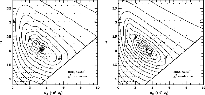
Figure 6: Contour plots of the $\chi^{2}$ that measures the quality of the fit to the combined HST, CHFT and WHT data, for orbit-superposition models with $i=90^{\circ}$ and $i=55^{\circ}$. The model parameters along the abscissa and ordinate are the BH mass $M_{\bullet}$ and the (V-band) mass-to-light ratio $\Upsilon$, respectively. The dots indicate models that were calculated, the contours were obtained through spline interpolation (the first three contours define the formal $68.3$, $95.4$ and (heavy contours) $99.73$ per cent confidence regions; subsequent contours are characterized by a factor two increase in $\Delta\chi^{2}$). The bottom right corner in each panel is a region for which no models were calculated. The labeled positions define models that are discussed in detail in the text and in subsequent figures. Models C and G provide the overall best fits.

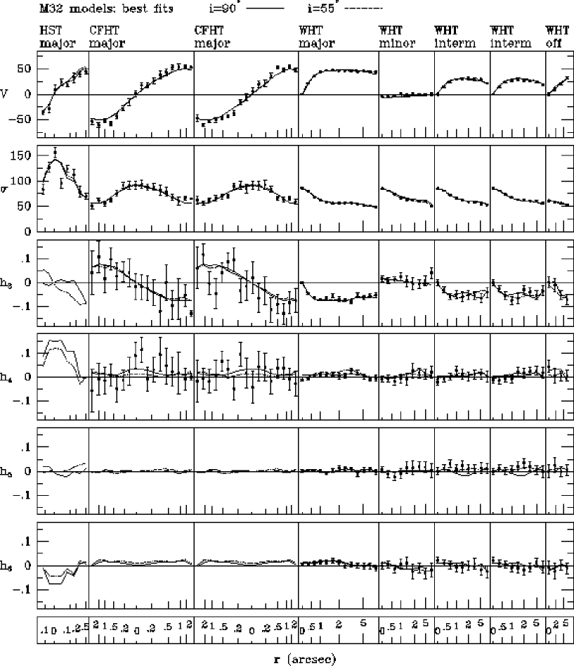
Figure 7: (continued).

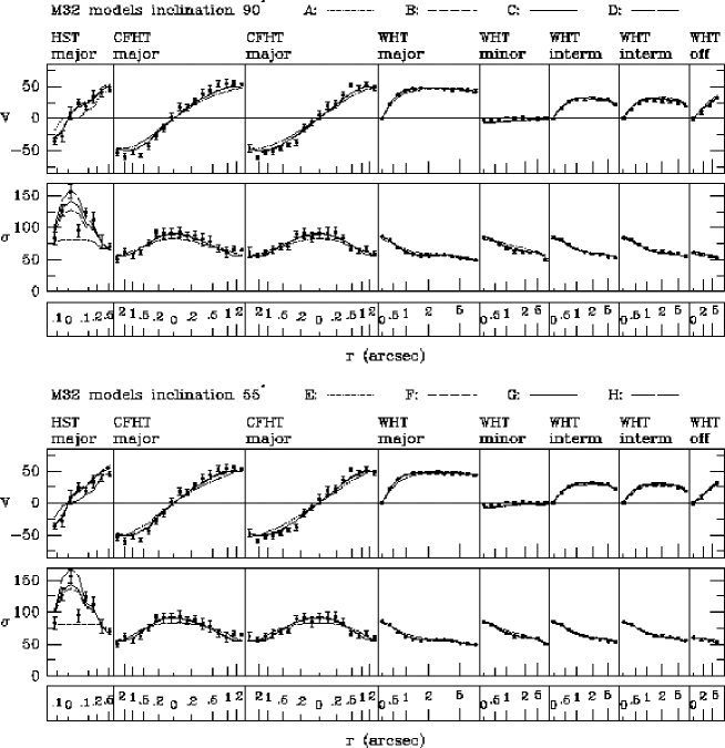
Figure 9: Predicted rotation velocities and velocity dispersions for the orbit-superposition models A–D (top panel) and E–H (bottom panel) defined in Figure 6. Models C&G are the overall best fits, models A&E are the best fits without a central dark mass, and models B&F and D&H are (approximately) the best-fitting models for $M_{\bullet}=1.9$ and $5.4\times 10^{6}\>{\rm M_{\odot}}$, respectively. The data are as in Figure 7. The models without a BH manage to fit the WHT data reasonably well, but are firmly ruled out by the HST data.

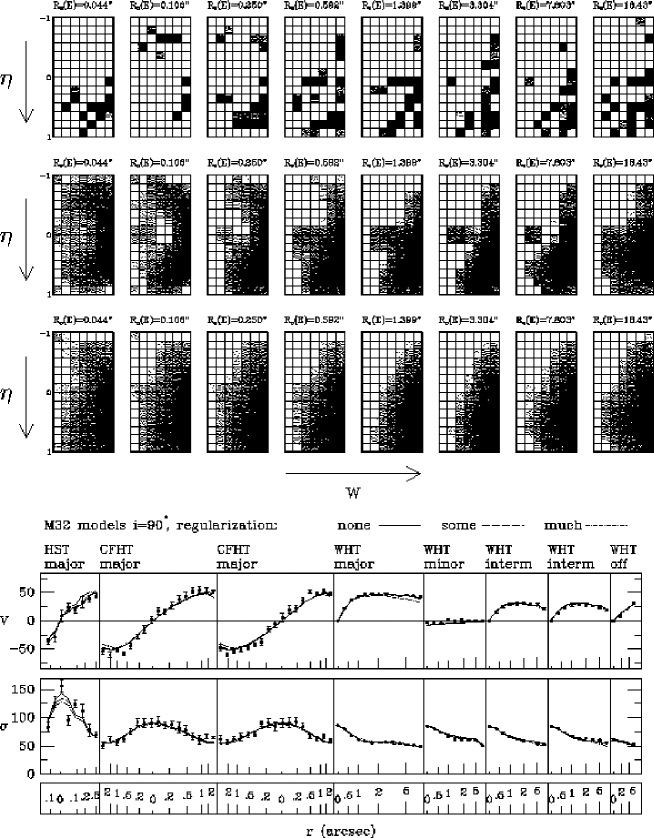
Figure 9: (continued).

We have studied three-integral models with dark central point-masses, i.e., $\epsilon=0$ in equation (2). There are then three free model parameters: the inclination $i$, the mass-to-light ratio $\Upsilon$, and the BH mass $M_{\bullet}$. The parameter space must be explored through separate sets of orbit libraries. As for the two-integral models, we have studied only two, widely spaced, inclinations: $i=90^{\circ}$ and $i=55^{\circ}$. For each inclination we have sampled the physically interesting range of $(\Upsilon,M_{\bullet})$ combinations. For each $(\Upsilon,M_{\bullet})$ combination we determined the orbital weights (and hence the dynamical structure) that best fit the data, and the corresponding goodness-of-fit quantity $\chi^{2}(\Upsilon,M_{\bullet})$. All available HST/FOS, CFHT and WHT data were included as kinematical constraints on the models. Older kinematical data for M32 were not included because of their lower spatial resolution and/or poorer sky coverage. In total, each NNLS fit had 1960 orbits to fit 782 constraints: 366 self-consistency constraints, and 416 kinematical constraints (for 86 positions on the projected plane of the galaxy). We focus primarily (Figures 6–9) on models without additional constraints that enforce smoothness in integral-space. This is a sufficient and conservative approach for addressing the primary question of our paper: which models are ruled out by the M32 data? If the data cannot even be fit with an arbitrarily unsmooth DF, they certainly cannot be fit with a smooth DF.

6.2 Data-model comparison

Figure 6 shows the main result: contour plots of $\chi^{2}(\Upsilon,M_{\bullet})$ for both inclinations that were studied. The displayed $\chi^{2}$ measures the quality of the fit to the kinematical constraints only; the actual NNLS fits were done to both the kinematical and the self-consistency constraints, but contour plots of the total $\chi^{2}$ look similar. The overall minimum $\chi^{2}$ values are obtained for: $\Upsilon=2.1$ and $M_{\bullet}=3.4\times 10^{6}\>{\rm M_{\odot}}$ for $i=90^{\circ}$; and $\Upsilon=2.0$ and $M_{\bullet}=3.2\times 10^{6}\>{\rm M_{\odot}}$ for $i=55^{\circ}$.

Figure 7 compares the kinematical predictions of the best-fitting edge-on and $i=55^{\circ}$ models to the data. Two problems with the data must be taken into account when assessing the quality of the fit. First, the HST velocity dispersions show a scatter between some neighboring points that is much larger than the formal errors, most likely due to some unknown systematic effect. The models cannot be expected to reproduce this. Second, the CFHT rotation velocities at radii $\gtrsim 0.5^{\prime\prime}$ exceed the WHT measurements by an amount which cannot be attributed to differences in spatial resolution, but must be due to some unknown systematic error in either of the two data sets. The WHT data have the smallest error bars, and therefore receive most weight in the NNLS fit. As a result, the models tend to underpredict the CFHT rotation curve.

These systematic problems with the data preclude the use of $\chi^{2}$ as a meaningful statistic to assess which models provide an acceptable fit: if the observations themselves are not mutually consistent, then clearly no model can be statistically consistent with all of them. Although the use of any statistical test is suspect in the presence of systematic errors, one may still assign confidence regions on the model parameters by using the relative likelihood statistic $\Delta\chi^{2}\equiv\chi^{2}-\chi^{2}_{\rm min}$. This statistic merely measures which parameter combinations provide an equally good (or bad) fit as the one(s) that yield the minimum $\chi^{2}$. If we assume that the observational errors are normally distributed (which, as mentioned, is likely to be an oversimplification), then $\Delta\chi^{2}$ follows a $\chi^{2}$ probability distribution with the number of degrees of freedom equal to the number of model parameters (Press et al. 1992).

The best-fitting edge-on model in Figure 7 has $\chi^{2}=690.0$ while the best-fitting $i=55^{\circ}$ model has $\chi^{2}=602.5$, both for $N=416$ degrees of freedom. The fact that $\chi^{2}>N$, even for these optimum fits, is due primarily to the systematic errors in the data. To the eye, the models appear to fit the data as well as could be hoped for. The $\chi^{2}$ values do indicate that the $i=55^{\circ}$ model provides a significantly better fit than the edge-on model, implying that M32 is not seen edge-on. However, the results presented here do not allow us to derive the actual inclination of M32. That would require a detailed study of the entire range of possible inclinations, which would be more computer-intensive. The important conclusion in the present context is that the topology of the $\chi^{2}$ contours in Figure 6 is virtually identical for both inclinations: the allowed range for $M_{\bullet}$ is therefore uninfluenced by our ignorance of the true inclination of M32.

The $\Delta\chi^{2}$ statistic was used to assign confidence values to the contours in Figure 6. At the $68.3$ per cent confidence level ($1\sigma$ for a Gaussian probability distribution), the allowed $M_{\bullet}$ fall in the range $(3.2$–$3.5)\times 10^{6}\>{\rm M_{\odot}}$ for $i=90^{\circ}$, and in the range $(3.1$–$3.4)\times 10^{6}\>{\rm M_{\odot}}$ for $i=55^{\circ}$. At the $99.73$ per cent confidence level ($3\sigma$ for a Gaussian probability distribution), they fall in the ranges $(2.5$–$3.7)\times 10^{6}\>{\rm M_{\odot}}$ and $(2.3$–$3.9)\times 10^{6}\>{\rm M_{\odot}}$, respectively. In reality, small numerical errors in the models might have distorted the $\chi^{2}$ contours. We address this issue in Appendix A. Any numerical errors are small enough that they have no influence on our conclusion that models without a dark mass are firmly ruled out. However, the possibility of small numerical errors does increase the confidence bands on $M_{\bullet}$. Based on the analysis in Appendix A, we conclude that $M_{\bullet}=(3.4\pm 0.7)\times 10^{6}\>{\rm M_{\odot}}$ at $68.3$ per cent confidence, and $M_{\bullet}=(3.4\pm 1.6)\times 10^{6}\>{\rm M_{\odot}}$ at $99.73$ per cent confidence. These estimates take into account both the observational errors in the data and possible numerical errors in the models, and are valid for both inclinations that were studied.

Figure 9 compares the model predictions to the observed rotation velocities and velocity dispersions for all the models labeled in Figure 6. Models C&G are the overall best fits for the two inclinations. Models B&F and D&H are (approximately) the best-fitting models for $M_{\bullet}=1.9$ and $5.4\times 10^{6}\>{\rm M_{\odot}}$, respectively. The latter models are marginally ruled out at the $>99$% confidence level (cf. the above discussion), although to the eye they do appear to reproduce the main features of the data. They differ from the overall best-fitting models primarily in their predictions for the HST velocity dispersions. The differences in the predictions for the ground-based data are smaller (and invisible to the eye in Figure 9), but nonetheless more statistically significant because of the smaller error bars for these data. Models A&E, the best fits without a central dark mass, are indisputably ruled out. The main problem for these models is to fit the central peak in the velocity dispersion. They come rather close to fitting the WHT observations, and predict a central dispersion of $\sim 84\>{\rm km}\,{\rm s}^{-1}$. However, the models without a dark mass fail to reproduce the higher central dispersion of $\sim 91\pm 2\>{\rm km}\,{\rm s}^{-1}$ measured with the CFHT (although still only marginally), and don’t even come close to reproducing the HST dispersions, which exceed $100\>{\rm km}\,{\rm s}^{-1}$ in the central $0.1^{\prime\prime}$.

6.3 Smooth solutions

The top row in Figure 10 illustrates the orbital occupancies in integral space for the best-fitting edge-on model (model C). Only a small fraction of the orbits in the library is used to fit the constraints, while the remainder receives zero weight. This yields an equilibrium solution of the collisionless Boltzmann equation, but is not physically plausible.

Smoothness of the solutions in integral space can be enforced by adding linear regularization constraints to the problem (Zhao 1996; C97). We have explored this only in an ad hoc way, merely to be able to assess the effect of smoothness constraints on the resulting fit to the data. A model is defined as a set of masses $m(R_{\rm c},\eta,w)$ in integral space. For each point that is not on the boundary of the $(R_{\rm c},\eta,w)$ grid, we measure the smoothness of the model (Press et al. 1992; eq. [18.5.10]) through the second order divided differences (in each of the three variables, assuming for simplicity that the distances between adjacent grid points are equal in all directions) of the function $m(R_{\rm c},\eta,w)/m_{0}(R_{\rm c})$. The function $m_{0}(R_{\rm c})$ is a rough approximation to the energy dependence of the model, obtained, e.g., by studying the spherical isotropic limit of the given mass density. The regularization constraints are then that the divided differences should equal $0\pm\Delta$, where the ‘error’ $\Delta$ determines the amount of smoothing. Models with $\Delta\rightarrow\infty$ have no smoothing, while models with $\Delta\rightarrow 0$ force $m(R_{\rm c},\eta,w)/m_{0}(R_{\rm c})$ to be a linear function on the $(R_{\rm c},\eta,w)$ grid.

The second and third rows in Figure 10 show the integral space for model C with the addition of either a modest ($\Delta=5$) or a large ($\Delta=0.2$) amount of regularization in the NNLS fit, respectively. As the bottom panels show, the price paid for the increased smoothness is a somewhat poorer fit to the data. However, the fits are still quite good. This demonstrates that the good fits to the data shown in Figure 7 are not primarily the result of the use of implausible distributions in integral space. These distributions result from the numerical properties of the problem, but there also exist smooth solutions which provide similar fits.

6.4 Dynamical Structure

Figure 12 illustrates the dynamical structure of the edge-on models A–D and the $i=55^{\circ}$ models E–H. By contrast to the models with a BH, the models A&E without a BH invoke a large amount of radial motion in the central arcsec to produce a peak in the observed velocity dispersions (cf. Binney & Mamon 1982). The maximum allowed radial anisotropy in the models is determined by the observed rotation velocities in M32, because dynamical models predict lower values of $V/\sigma$ when they are more radially anisotropic (Richstone, Bower & Dressler 1990; de Bruijne, van der Marel & de Zeeuw 1996). Figure 9 shows that the allowed radial anisotropy is by far insufficient to fit the observed peak in the velocity dispersion profile without invoking a BH.

The models B–D and F–H, which represent the best fits for different potentials, all have a similar dynamical structure in that they are dominated by azimuthal motion. This is most pronounced for the intrinsically flatter $i=55^{\circ}$ models. It is not known what physical process could have produced this particular velocity ellipsoid shape in M32. The rightmost panels in Figure 12 show the velocity moments for $f(E,L_{z})$ models with the same gravitational potentials as models C&G. The $f(E,L_{z})$ models are similar to the best-fitting three-integral models, in that they have an excess of azimuthal motion. This is why they have been so successful in fitting ground-based data, including available VP shape parameters, and it shows that they provide a useful low-order approximation to the dynamical structure of M32. However, the $f(E,L_{z})$ models have $\langle v_{r}^{2}\rangle=\langle v_{\theta}^{2}\rangle$ by definition, in contrast to the inequality between $\langle v_{r}^{2}\rangle$ and $\langle v_{\theta}^{2}\rangle$ seen in the best-fitting three-integral models. This explains the finding of Section 4.2 that $f(E,L_{z})$ models cannot successfully reproduce all observed features of the kinematical data.

The second velocity moments $\langle v_{r}^{2}\rangle$ and $\langle v_{\theta}^{2}\rangle$ can be combined with the mixed moment $\langle v_{r}v_{\theta}\rangle$ to determine the tilt of the velocity ellipsoid in the meridional plane. For all the models A–D and E–H we found $\langle v_{r}v_{\theta}\rangle$ to be small, and the velocity ellipsoids are more closely aligned with spherical coordinate axes than with cylindrical coordinate axes (but they are not perfectly aligned with either). This is not uncommon in three-integral models for axisymmetric systems (e.g., Dejonghe & de Zeeuw 1988; Dehnen & Gerhard 1993; de Zeeuw, Evans & Schwarzschild 1996).

Figure 13 shows the quantity $\langle v_{\phi}\rangle\,/\,\langle v^{2}\rangle^{1/2}$ in the equatorial plane, for the models C and G. The inclined, and intrinsically flatter, model G rotates faster than the edge-on model C. The predictions for oblate isotropic rotator models ($\sigma_{r}=\sigma_{\theta}=\sigma_{\phi}$) are shown for comparison. The edge-on model C rotates faster than an oblate isotropic rotator model for radii $r\gtrsim 0.5^{\prime\prime}$; the inclined model G rotates slower than the oblate isotropic rotator model.

We have not attempted to derive confidence bands on the dynamical structure of M32. This is a much more difficult problem than the derivation of confidence bands on the model parameters $(M_{\bullet},\Upsilon)$, and is beyond the scope of the present paper.

7 Models with an extended dark nuclear object

The results in the previous section demonstrate that M32 must have a massive dark object in its nucleus. To obtain a limit on the size of this dark object, we have studied models in which it has a finite size $\sim\epsilon$ (cf. eq. [2]). Searching the parameter space of three-integral models with different $\epsilon$ is extremely computer-intensive. We have therefore restricted ourselves to $f(E,L_{z})$ models with extended dark objects. This is not likely to bias our conclusions, because the best-fitting three-integral models found in Section 6 are similar to two-integral models.

Figure 14 shows the predictions of edge-on $f(E,L_{z})$ models with extended nuclear dark objects, for two representative values of $M_{\bullet}$. As in the models of Section 4.1, the fraction $F$ of stars with $L_{z}>0$ in each model was chosen to best fit the rotation curve. By adjusting $F$, adequate fits to the rotation velocities can be obtained for most relevant models. Hence, only the velocity dispersions are shown in the figure. The predicted dispersions are typically constant or decreasing towards the center within the scale radius $\epsilon$. The HST data show a much higher velocity dispersion in the center than further out. Hence, the extension of any possible dark nuclear cluster cannot be large; Figure 14 suggests $\epsilon\lesssim 0.1^{\prime\prime}$. Figure 15 shows a contour plot of the quantity $\chi_{\sigma}^{2}$ (eq. [3]), measuring the quality of the model fit to the HST dispersion measurements, both for the edge-on case and for $i=55^{\circ}$. The best fit is obtained for $\epsilon=0$ (the point mass case discussed previously). The formal $99.73$ per cent confidence level (assuming Gaussian formal errors) rules out all models with $\epsilon\gtrsim 0.06^{\prime\prime}$, independent of the inclination. The models with the largest $\epsilon$ must have a total mass of at least $M_{\bullet}\approx 4\times 10^{6}\>{\rm M_{\odot}}$.

At the distance of M32, $1^{\prime\prime}=3.39\>{\rm pc}$. Hence, the upper limit on the scale radius corresponds to $\epsilon=0.20\>{\rm pc}$. Combined with a total mass in the cluster of $M_{\bullet}\approx 4\times 10^{6}\>{\rm M_{\odot}}$, this implies a central mass density of at least $\rho_{0}=1.1\times 10^{8}\>{\rm M_{\odot}}\>{\rm pc}^{-3}$. The half-mass radius of a Plummer model is $r_{\rm h}=1.30\epsilon$. Hence, there must be $\sim 2\times 10^{6}\>{\rm M_{\odot}}$ inside $r\lesssim 0.078^{\prime\prime}$. The total V-band luminosity inside this radius is $1\times 10^{5}\>{\rm L_{\odot}}$, implying a luminous mass of $2.5\times 10^{5}\>{\rm M_{\odot}}$. Hence, the ratio of the total mass to luminosity inside this radius must be $\gtrsim 22.5$.

The observed kinematics constrain only the amount of mass in the system, not whether this mass is luminous or dark. One can therefore fit the data equally well with models in which the average mass-to-light ratio $\Upsilon$ of the stellar population increases towards the nucleus, and in which there is no dark mass. We have not explicitly constructed such models, but it is clear from the preceding discussion that in such models $\Upsilon$ must rise from $\sim 2$ in the main body of the galaxy to $\gtrsim 20$ at $r\lesssim 0.1^{\prime\prime}$. Such a drastic variation in mass-to-light ratio would imply a strong change in the stellar population, accompanied by broad-band color gradients. The size of these gradients depends on the actual stellar population mix, which is unknown. However, one may use the properties of main sequence stars as a guideline. For these, a change in $\Upsilon$ from $2$ to $20$ implies color changes $\Delta(U-B)\approx 0.9$, $\Delta(B-V)\approx 0.6$, and $\Delta(V-I)\approx 0.8$ (using the tables of stellar properties in Allen 1973). Such variations between $0.1^{\prime\prime}$ and $1^{\prime\prime}$ should have been obvious in photometric observations. However, neither subarcsec resolution ground-based imaging (Lugger et al. 1992) nor pre-refurbishment HST imaging (Crane et al. 1993) have revealed any significant color gradients in the central arcsec of M32. Post-refurbishment HST observations (Lauer et al., private communication) also do not show strong color gradients. Thus, the nuclear mass concentration in M32 cannot be due merely to a change in the mix of ordinary stars in the nuclear region.

The absence of observed color gradients does not exclude the possibility of nuclear concentrations of brown dwarfs, white dwarfs, neutron stars, or stellar-mass BHs in M32. However, at high densities, such clusters of dark objects are not stable over a Hubble time. This was discussed by Goodman & Lee (1989), and their arguments were updated and extended in van der Marel et al. (1997a). The latter paper shows that the new HST limit on the density of dark material in M32 rules out all but the most implausible clusters, leaving a single massive BH as the most likely interpretation of the data.

The kinematical predictions of our models depend on the assumed Plummer form of the extended dark object. If it is a cluster of collapsed objects, this distributed dark mass may itself be cusped (e.g., Gerhard 1994). However, the limit on $\epsilon$ results from the fact that the dispersion of stars with mass density (1) in a Plummer potential does not have a (strong) central peak. This property is common to many alternative types of models, such as those of King (e.g., Binney & Tremaine 1987), Hernquist (1990) and Jaffe (1983). These all produce constant or decreasing dispersions inside their scale radius, as does the Plummer model. Hence, the upper bound on $\epsilon$ derived here is likely to be generic to most plausible density profiles for the extended dark object. In addition, King, Jaffe and Hernquist models are more centrally condensed than Plummer models, and would therefore require dark clusters of even higher central densities to fit the data.

8 Conclusions and discussion

8.1 Summary of results

The main bottlenecks in proving the presence of nuclear BHs in quiescent galaxies from stellar kinematical data have long been: (i) the restricted spatial resolution of ground-based data; and (ii) lack of sufficiently general dynamical models to rule out constant mass-to-light ratio models beyond doubt. The HST now provides spectra of superior spatial resolution. To fully exploit the potential of these new data it is imperative to improve the modeling techniques that have been used in the past decade. The situation is considerably more complicated than for gas disks in (active) galaxies, where the assumption of simple circular orbits is often adequate. Interpretation of stellar kinematical data for flattened elliptical galaxies ideally requires axisymmetric (or even better, triaxial) dynamical models with completely general three-integral distribution functions. Such models have not previously been constructed for any stellar kinematical BH candidate galaxy. We therefore developed a technique for the construction of such axisymmetric models, and used it to interpret our HST data for M32.

To guide the construction and interpretation of the three-integral models we first compared the new HST data to the predictions of $f(E,L_{z})$ models, which have been used extensively to interpret ground-based M32 data. Such models have the advantage that the DF can be calculated semi-analytically, but have the disadvantage of having a special dynamical structure, with $\sigma_{r}=\sigma_{\theta}$ everywhere. There is no a priori reason why any galaxy should have this property. However, the fact that $f(E,L_{z})$ models fit the observed VP shapes inferred from ground-based data to within $\sim 2$% (in terms of deviations from a Gaussian), suggested that the M32 DF might in fact be close to the form $f(E,L_{z})$. We find here that $f(E,L_{z})$ models for M32 can also fit the new HST data, and that this requires the presence of a nuclear dark mass, as was the case for the ground-based data. However, the best fitting dark mass of $M_{\bullet}=(2.5$–$4.5)\times 10^{6}\>{\rm M_{\odot}}$ is larger than the $M_{\bullet}=(2$–$3)\times 10^{6}\>{\rm M_{\odot}}$ that best fits the $\sim 0.5^{\prime\prime}$ spatial resolution data from the CFHT, and is even more different from the $M_{\bullet}=(1.5$–$2)\times 10^{6}\>{\rm M_{\odot}}$ that best-fits the $\sim 0.9^{\prime\prime}$ spatial resolution data from the WHT. Thus, under the assumption of an $f(E,L_{z})$ DF, the different data sets cannot be fit with the same $M_{\bullet}$. This indicates that the M32 DF is not of the form $f(E,L_{z})$, although it might be close to it.

To obtain a model-independent estimate of the best-fitting $M_{\bullet}$, and to firmly rule out models without any dark mass, it is necessary to study more general three-integral models. We have made such models for M32, both with and without central BHs, and for various possible values of the average mass-to-light ratio $\Upsilon$ of the stellar population. The models were constructed to fit all available kinematical HST, CFHT and WHT data, and the acceptability of each model was assessed through the $\chi^{2}$ of its fit to the data. The models demonstrate explicitly for the first time that there is no axisymmetric constant mass-to-light ratio model that can fit the kinematical data without invoking the presence of a nuclear dark mass, independent of the dynamical structure of M32. A nuclear dark point mass of $M_{\bullet}=(3.4\pm 1.6)\times 10^{6}\>{\rm M_{\odot}}$ is required (with $1\sigma$ and $3\sigma$ error bars of $0.7\times 10^{6}\>{\rm M_{\odot}}$ and $1.6\times 10^{6}\>{\rm M_{\odot}}$, respectively, which includes the possible effect of small numerical errors in the models). This mass is similar to that quoted by most previous papers, but the confidence on the detection of a nuclear dark mass in M32 is now much higher. Constant mass-to-light ratio models still come very close to fitting the ground-based data, and only the new HST data make the case for a nuclear dark mass clear-cut.

The inclination of M32 cannot be inferred from the available surface photometry, and is therefore a free parameter in the modeling. Ideally one would like to construct dynamical models for all possible inclinations (which would be very computer-intensive) and determine the inclination that best fits the kinematical data. Here we have taken the more modest approach of constructing models for only two representative inclinations: $i=90^{\circ}$ (edge-on) and $i=55^{\circ}$. The intrinsic axial ratios for these inclinations are $q=0.73$ and $q=0.55$, respectively. The three-integral $i=55^{\circ}$ models provide a better fit than the edge-on models, which suggests that M32 is not seen edge-on. However, the allowed range for $M_{\bullet}$ does not depend sensitively on the assumed inclination: models with no central dark mass are firmly ruled out for both inclinations. So even though a more detailed study of the full inclination range for M32 would improve our knowledge of the true inclination and intrinsic axial ratio of M32, it would probably not change significantly the constraints on the central dark mass.

The best-fitting three-integral models are similar to $f(E,L_{z})$ models in that they have an excess of azimuthal motion. This is why they have been so successful in fitting ground-based data, including available VP shape parameters, and it confirms that they provide a useful low-order approximation to the dynamical structure of M32. However, $f(E,L_{z})$ models do have $\sigma_{r}\equiv\sigma_{\theta}$. This does not reproduce the inequality between $\sigma_{r}$ and $\sigma_{\theta}$, nor the modest tilt of the velocity ellipsoid indicated by the small $\langle v_{r}v_{\theta}\rangle$ term, seen in the best-fitting three-integral models. This is why $f(E,L_{z})$ models cannot successfully explain all observed features of the kinematical data.

To constrain the size of the dark object in M32 we have constructed $f(E,L_{z})$ models with an extended dark nuclear object. These show that the HST data put an upper limit of $0.08^{\prime\prime}=0.26\>{\rm pc}$ on the half-mass radius of the nuclear dark object, implying a central density exceeding $1\times 10^{8}\>{\rm M_{\odot}}\>{\rm pc}^{-3}$. This limit on the density of dark material in M32 essentially rules out nuclear clusters of planets, brown dwarfs, white dwarfs, neutron stars, or smaller mass BHs (van der Marel 1997a). The absence of color gradients in the central arcsec of M32 implies that the nuclear mass concentration can also not be attributed to a stellar population gradient. A single massive nuclear BH therefore provides the most plausible interpretation of the data.

8.2 Dynamical stability

Axisymmetric dynamical models with a nuclear BH provide an excellent fit to all available kinematical data for M32. However, to be physically meaningful, the models must also be dynamically stable. In van der Marel, Sigurdsson & Hernquist (1997c) we presented N-body simulations of the $f(E,L_{z})$ models for M32. The models were found to be completely stable, both for $i=90^{\circ}$ and for $i=55^{\circ}$. This shows that dynamical stability is not a problem for the models, and that the inclination of M32 cannot be meaningfully constrained through stability arguments. We have not evolved N-body models for the best-fitting three-integral models, but we expect these models to be stable as well, given their similarity to $f(E,L_{z})$ models.

8.3 Dynamical relaxation

The two-body relaxation time in M32 can be estimated as in, e.g., Binney & Tremaine (1987; eq. [8-71]). Using the relevant quantities for our best-fitting dynamical model, we find for solar mass stars in the central cusp ($r\lesssim 0.5^{\prime\prime}$) that $t_{\rm relax}\approx 3\times 10^{9}\>(r/0.1^{\prime\prime})^{-0.065}\>{\rm yr}$. The time scale for ‘resonant relaxation’ (Rauch & Tremaine 1996) is of the same order. The central cusp must therefore be evolving secularly over a Hubble time. However, the diffusion of stars in phase space is slow enough that one may assume the evolution to be through a sequence of quasi-equilibrium models. This justifies our approach of modeling M32 as a collisionless equilibrium system. Studies of the secular evolution of the M32 cusp will be interesting, but will not change the need for a nuclear dark object. In fact, the process of dynamical relaxation supports the presence of a dark object: without a dark object the relaxation would proceed at a much more rapid rate that is difficult to reconcile with observations (Lauer et al. 1992).

8.4 Triaxiality

One remaining uncertainty in our dynamical modeling is the possibility of triaxiality. After the step from spherical models to axisymmetric models, triaxial models are the obvious next step. However, there are several reasons to believe that for M32 this additional step will be less important. First, M32 is known not to be spherical, but there is no reason why it cannot be axisymmetric. There is no significant isophote twisting in M32, and no minor axis rotation. This does not mean that M32 cannot be triaxial (we might be observing it from one of the principal planes), but it also does not mean that M32 needs to be triaxial. Second, spherical constant mass-to-light ratio models (without a nuclear dark mass) for ground-based M32 data failed to fit by only a few $\>{\rm km}\,{\rm s}^{-1}$, and it was quite conceivable that axisymmetry could fix this (which it did, cf. Figure 17 below). However, axisymmetric constant mass-to-light ratio models for the new HST data fail to fit the nuclear velocity dispersion by $>50$ km/s, and this cannot likely be fixed through triaxiality. Third, theoretical arguments suggest that strongly triaxial models with density cusps as steep as in M32 may not be stable, owing to the fact that regular box-orbits are replaced by boxlets and irregular orbits that may not be able to sustain a triaxial shape (Binney & Gerhard 1985; Merritt & Fridman 1996; Merritt & Valluri 1996; see also the review by de Zeeuw 1996). Rapidly-rotating low-luminosity elliptical galaxies like M32 always have steep power-law cusps (Faber et al. 1997), and may therefore be axisymmetric as a class (de Zeeuw & Carollo 1996). This is consistent with statistical studies of their intrinsic shapes (e.g., Merritt & Tremblay 1996). So, apart from the fact that triaxiality is unlikely to remove the need for a central dark object in M32, it may even be so that M32 cannot be significantly triaxial.

8.5 Adiabatic black hole growth

The growth of a black hole into a stellar system is adiabatic if it occurs over a time scale that is ‘long’ (see Sigurdsson, Quinlan, & Hernquist 1995 for a quantitative discussion) compared to the typical orbital period of the stars. For the case of M32, the black hole formation can be considered adiabatic if it took at least $10^{6}\>{\rm yr}$. Young (1980) studied the adiabatic growth of BHs in spherical isothermal models with central density $\rho_{0}$ and core radius $r_{0}$. The BH growth leaves the mass density at large radii unchanged, but induces a central cusp $\rho\propto r^{-1.5}$ for $r\rightarrow 0$. The form of the density profile at intermediate radii is determined by the dimensionless parameter ${\overline{M}}_{\bullet}\equiv M_{\bullet}/[{4\over 3}\pi\rho_{0}r_{0}^{3}]$, which measures the ratio of the BH mass to the initial core mass. Lauer et al. (1992) showed that the shape of the M32 brightness profile measured with HST can be well fit with ${\overline{M}}_{\bullet}=0.33\pm 0.11$. The radial and density normalization implied by the data are then $r_{0}=3.0\>{\rm pc}$ and $\rho_{0}=(4.2\times 10^{4})\Upsilon\>{\rm M_{\odot}}\>{\rm pc}^{-3}$. This photometric model therefore implies that $M_{\bullet}/\Upsilon=(1.6\pm 0.5)\times 10^{6}\>{\rm M_{\odot}}$. Although this result depends somewhat on the assumed isothermality of the initial distribution (Quinlan, Hernquist & Sigurdsson 1995), it is quite remarkable that our best-fitting dynamical models have exactly $M_{\bullet}/\Upsilon=1.6\times 10^{6}\>{\rm M_{\odot}}$, for both inclinations that we studied. The M32 data are therefore fully consistent with the presence of a BH that grew adiabatically into a pre-existing core. This is similar to the situation for M87 (cf. Young et al. 1978; Harms et al. 1994).

Lee & Goodman (1989) extended Young’s calculations to the case of rotating models. For the value of ${\overline{M}}_{\bullet}$ implied by the photometry, their models predict a profile of $\langle v_{\phi}\rangle\,/\,\langle v^{2}\rangle^{1/2}$ that is approximately flat with radius (with amplitude fixed by the axial ratio of the system). However, this result depends very sensitively on the assumed rotation law of the initial model. The radial variations in $\langle v_{\phi}\rangle\,/\,\langle v^{2}\rangle^{1/2}$ seen in our best-fitting models (Figure 13) are probably equally consistent with the adiabatic growth hypothesis.

8.6 Tidal disruption of stars

A star of mass $m_{\star}$ and radius $r_{\star}$ on a circular orbit of radius $r$ will be tidally disrupted if $r\lesssim r_{\rm t}\equiv(2M_{\bullet}/m_{\star})^{1/3}r_{\star}$ (e.g., Binney & Petit 1988). Thus, disruption of a solar type star by the BH in M32 will occur inside $r_{\rm t}=4.2\times 10^{-6}\>{\rm pc}=1.2\times 10^{-6}$ arcsec. A disruption event will be highly luminous, but is not predicted to occur more often than once every $10^{4}\>{\rm yr}$ (Rees 1988). The minimum pericenter distance for a star with given $(E,L_{z})$ in a Kepler potential is $r_{\rm p,min}=R_{\rm c}(E)\>(1-\sqrt{1-\eta^{2}})$, where as before, $R_{\rm c}$ is the radius of the circular orbit at the given energy and $\eta\equiv L_{z}/L_{\rm max}(E)$. The kinematical data for M32 only meaningfully constrain the DF for energies with $R_{\rm c}(E)\gtrsim 0.1^{\prime\prime}$. For $R_{\rm c}(E)=0.1^{\prime\prime}$, only stars with $|\eta|<5\times 10^{-3}$ have $r_{\rm p,min}<r_{t}$. The data do not constrain variations in the DF over such a small range in $\eta$, and our dynamical models therefore cannot address the existence and properties of the so-called ‘loss cone’ (Frank & Rees 1976; Lightman & Shapiro 1977). For the $\eta$-grid that we have employed, all solar type stars on orbits with $R_{\rm c}(E)>0.1^{\prime\prime}$ have $r_{\rm p,min}>2\times 10^{2}\>r_{t}$. Even giants with $r_{\star}\approx 10^{2}r_{\odot}$ have $r_{\rm p,min}>r_{t}$. This justifies our neglect of tidal disruption in the orbit calculations.

8.7 Accretion onto the black hole

An interesting question is why BHs in quiescent galaxies aren’t more luminous (e.g., Kormendy & Richstone 1995). For M32, the total X-ray luminosity is $L_{\rm X}\approx 10^{38}\>{\rm erg}\,{\rm s}^{-1}$ (Eskridge, White & Davis 1996), the far infrared luminosity is $L_{\rm FIR}<3\times 10^{36}\>{\rm erg}\,{\rm s}^{-1}$ (Knapp et al. 1989), and for the $6\>{\rm cm}$ radio emission $\nu L_{\nu}<3\times 10^{33}\>{\rm erg}\,{\rm s}^{-1}$ (Roberts et al. 1991). Part or all of the observed X-ray emission may be due to low-mass X-ray binaries, so the total luminosity due to accretion onto the BH in M32 is $L_{\rm acc}<10^{38}\>{\rm erg}\,{\rm s}^{-1}$. By contrast, the Eddington luminosity of the BH is $L_{\rm Edd}=4.3\times 10^{44}\>{\rm erg}\,{\rm s}^{-1}$. For a canonical mass-loss rate of $1.5\>{\rm M_{\odot}}(10^{11}\>{\rm L_{\odot}})^{-1}\>{\rm yr}^{-1}$ (Faber & Gallagher 1976), the stars that are bound to the BH in M32 shed $1\times 10^{-4}\>{\rm M_{\odot}}\>{\rm yr}^{-1}$ of gas as a result of normal stellar evolution. If a fraction $f$ of this gas is steadily accreted with efficiency $\epsilon$, it produces a luminosity $L_{\rm acc}=\epsilon f\>(6.7\times 10^{42})\>{\rm erg}\,{\rm s}^{-1}$. Thus either the accretion fraction $f$ or the accretion efficiency $\epsilon$ must be very small in M32. Thin disk accretion with $\epsilon\approx 0.1$ requires $f<1.5\times 10^{-4}$, which is possible (the accretion fraction is difficult to predict theoretically, because it depends on the hydrodynamics of the stellar winds that shed the gas), but may be implausibly low. Instead, it appears more likely that $\epsilon$ is small, since there is a family of ‘advection dominated’ accretion solutions that naturally predict such low efficiencies. Models of this type successfully explain the ‘micro-activity’ of the BH (Sgr A${}^{{}^{\star}}$) in our own Galaxy (Narayan, Yi & Mahadevan 1995). In a typical accretion model of this type (Narayan & Yi 1995, their Fig. 11), $f\lesssim 0.16$ suffices to explain the upper bound on $L_{\rm acc}$ for M32.

8.8 Forthcoming observations

Future observations of M32 will include spectra with the new long-slit HST spectrograph STIS. These will provide significantly better sky coverage than our FOS data, but the spatial resolution will be similar. The high-resolution HST data can be complemented with that from fully two-dimensional ground-based spectrographs, such as OASIS on the CFHT and SAURON on the WHT. These combined data will yield improved constraints on the BH mass, on the orbital structure and inclination of M32, and on possible deviations from axisymmetry.

Appendix A $\chi^{2}$ topology for orbit-superposition models

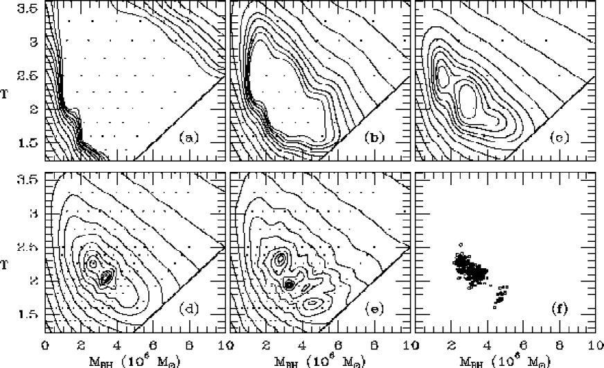
Figure 16: Contour plots of $\chi^{2}(M_{\bullet},\Upsilon)$ for edge-on orbit superposition models constructed to fit: (a) the major axis WHT $V$ and $\sigma$ measurements; (b) all major axis WHT measurements, including VP shapes; (c) all WHT measurements, including various position angles; (d) all WHT, CFHT and HST data (same as Figure 6). Contours are defined as in Figure 6. Heavy contours show the formal $99.73$% confidence regions. Panel (e) shows how the contours in panel (d) are modified if random errors are added to the predictions for each data point, to simulate numerical errors in the models. Panel (f) shows for 100 simulations as in panel (e) the position of the $\chi^{2}$ minimum (solid symbols), and the lowest and highest $M_{\bullet}$ that fall within a $99.73$% confidence contour (open symbols). These simulations show that numerical errors cannot be responsible for the fact that models with either $M_{\bullet}<1.8\times 10^{6}\>{\rm M_{\odot}}$ or $M_{\bullet}>5.0\times 10^{6}\>{\rm M_{\odot}}$ fail to fit the data at this confidence level.

In this Appendix we discuss the topology of the $\chi^{2}(\Upsilon,M_{\bullet})$ contours for the edge-on orbit-superposition models. The top panels of Figure 16 show the $\chi^{2}$ contours when only (subsets of) the ground-based WHT data are included in the fit. These panels can be compared to Figure 16d, which shows the contours for the case in which all WHT, CFHT and HST data are included.

Figure 16a shows the $\chi^{2}$ contours when only the major axis $V$ and $\sigma$ WHT measurements are fit. Binney & Mamon (1982) showed that a large range of gravitational potentials can fit any given observed velocity dispersion profile. The valley seen in the $\chi^{2}$ contours is a consequence of this: it outlines a one-parameter family of models that can fit the data with different velocity dispersion anisotropy. For a non-rotating spherical system, only models that require negative second velocity moments are ruled out. For a rotating system like M32, the observed rotation rate sets additional limits on the allowed radial anisotropy. For the case of the major axis $V$ and $\sigma$ WHT measurements, a no-BH model is just marginally acceptable at $99.73$ per cent confidence, cf. Figure 16a. For the lower-spatial resolution major axis $V$ and $\sigma$ measurements of Dressler & Richstone (1988) such a model is entirely acceptable. Figure 17 compares the predictions of the best-fit axisymmetric orbit-superposition model without a BH to their data. Richstone, Bower & Dressler (1990) concluded that these data could not be fit by any spherical model without a BH. This is because spherical models allow less rotation, and therefore failed to fit the observed rotation velocities. This underscores the importance of making axisymmetric models for flattened galaxies like M32.

VP shape measurements provide independent constraints on the velocity dispersion anisotropy. Figure 16b shows the $\chi^{2}$ contours for edge-on orbit-superposition models when not only the WHT major axis $V$ and $\sigma$ measurements are fit, but also the major axis VP shape measurements. With the inclusion of the VP shapes, models without a BH are ruled out. Figure 16c shows the $\chi^{2}$ contours when also the WHT measurements along other position angles are included, which contracts the allowed $M_{\bullet}$ range to $(1.1$–$5.1)\times 10^{6}\>{\rm M_{\odot}}$ at the formal $99.73$ per cent confidence level. The WHT data by themselves therefore rule out axisymmetric models without a BH. However, the models without a BH still come very close to fitting the data, and, e.g., fail to fit the central velocity dispersion by only 1–2$\>{\rm km}\,{\rm s}^{-1}$ (cf. Figure 9). So one cannot make a particularly strong claim for a BH on the basis of the WHT data alone, because it is conceivable that the fit could be improved with, e.g., only a minor amount of triaxiality. The same holds for the CFHT data, but the new HST data do make the case for a BH in M32 clear-cut.

The contours for the case in which all the available WHT, CFHT and HST kinematical data are included in the fit (Figure 16d) show one global $\chi^{2}$ minimum, and a second local minimum. The presence of a global minimum does not necessarily imply that the combined data constrain a single best-fit potential. It might be that there is a small range of potentials that all fit equally well, but that such a range of constant $\chi^{2}$ would not be evident due to the finite numerical accuracy of our technique. In Figure 16e we show explicitly how the topology of the $\chi^{2}$ contours might have been influenced by the possibility of small numerical errors in our models. It was obtained from Figure 16d by recalculating the $\chi^{2}$ contours after adding a random error $\Delta V,\sigma\in[-2,2]$ km/s and $\Delta h_{i}\in[-0.01,0.01]$ (cf. Section 5) to the prediction for each data point, for each $(\Upsilon,M_{\bullet})$ combination. The results show that numerical errors can indeed influence the $\chi^{2}$ contours near the $\chi^{2}$ minimum. Thus, the second minimum in Figure 16d might be the result of numerical inaccuracies in our technique. However, the numerical errors are small enough that they only have a negligible effect on the overall $\chi^{2}$ topology. In particular, models without a dark mass remain firmly ruled out.

To assess the possible effect of numerical errors on the confidence bands for $M_{\bullet}$, we constructed 100 figures like Figure 16e using different random realizations. For each we determined the position of the $\chi^{2}$ minimum, and the minimum and maximum $M_{\bullet}$ for which there is an $\Upsilon$ such that the model with $(M_{\bullet},\Upsilon)$ falls within the $99.73$ per cent confidence region. The results are plotted in Figure 16f. All allowed $M_{\bullet}$ values fall in the range $M_{\bullet}=(1.8$–$5.0)\times 10^{6}\>{\rm M_{\odot}}$. Thus, $M_{\bullet}=(3.4\pm 1.6)\times 10^{6}\>{\rm M_{\odot}}$ at $99.73$ per cent confidence. Similar experiments show that $M_{\bullet}=(3.4\pm 0.7)\times 10^{6}\>{\rm M_{\odot}}$ at $68.3$ per cent confidence. Experiments for $i=55^{\circ}$ produced similar results, and mass ranges that were either the same or slightly smaller. Thus, we conclude that the $1\sigma$ and $3\sigma$ errors on the estimated $M_{\bullet}=3.4\times 10^{6}\>{\rm M_{\odot}}$, are $0.7$ and $1.6\times 10^{6}\>{\rm M_{\odot}}$, respectively.

Figure 1: Data points are observations of the M32 major axis V-band surface brightness from Lauer et al. (1992), Peletier (1993) and Kent (1987). The R-band data from Kent and Peletier were transformed to the V-band by assuming a constant V$-$R color. The differences between the data sets at large radii are due to uncertainties in the sky subtraction. Measurements are not plotted at radii where the PSF introduces large uncertainties ($\sim 0.1^{\prime\prime}$ for the Lauer et al. HST data, $\sim 2^{\prime\prime}$ for the ground-based data). The solid curve is the brightness profile for the axisymmetric luminous density model used in the present paper. The dashed curve is the profile for the model used by van der Marel et al. (1994b) and Qian et al. (1995).

Figure 2: Data points show the rotation velocities $V$ and velocity dispersions $\sigma$ derived from the HST/FOS data of Paper I, and from the ground based WHT and CFHT data of van der Marel et al. (1994a) and Bender, Kormendy & Dehnen (1996). Errors for the ground-based data are $\sim 1\>{\rm km}\,{\rm s}^{-1}$ for the WHT data and $\sim 6\>{\rm km}\,{\rm s}^{-1}$ for the CFHT data, but are not plotted for clarity. The abscissa $r$ is the major axis distance. Curves show the predictions for the HST setup of edge-on $f(E,L_{z})$ models with no nuclear dark mass (dashed curves) and with nuclear point masses (BHs) of 1, 2, 3, 4, 5 and $6\times 10^{6}\>{\rm M_{\odot}}$ (solid curves). Models with $M_{\bullet}\approx(3\pm 1)\times 10^{6}\>{\rm M_{\odot}}$ best reproduce the trend in the observed dispersions.

Figure 3: The relative RMS velocity dispersion residual $\chi_{\sigma,{\rm RMS}}$ for edge-on $f(E,L_{z})$ models with nuclear point masses, as function of $M_{\bullet}$. Results are shown for the HST dispersion measurements of Paper I, and for the ground-based WHT and CFHT measurements. The $\chi_{\sigma,{\rm RMS}}$ for the best fit to the WHT data is larger than for the CFHT data, because the WHT data have much smaller errors (such that differences between the predictions and the data are statistically more significant). The symbols in the box mark the position of the best-fitting $M_{\bullet}$ for each data set and its formal $1\sigma$ error bar (the latter is determined not only by the curvature at the $\chi_{\sigma,{\rm RMS}}$ minimum, but also by the number of data points, which is different for each data set). Models with $M_{\bullet}\approx 3\times 10^{6}\>{\rm M_{\odot}}$ best fit the HST and the CFHT data. The WHT data are not well fitted by this $M_{\bullet}$. The fact that data of different spatial resolution cannot be fit with the same $M_{\bullet}$ implies that M32 does not have a DF of the form $f=f(E,L_{z})$.

Figure 4: Horizontally hatched regions show the average velocity dispersion and its $1\sigma$ error for those HST, CFHT and WHT observations with the aperture center within $0.1^{\prime\prime}$ from the M32 nucleus. Curves show the predictions for edge-on $f(E,L_{z})$ models with nuclear point masses, as function of $M_{\bullet}$. Models with no nuclear dark mass are ruled out under the $f(E,L_{z})$ hypothesis. Models with nuclear point masses reproduce the increase in the observed nuclear velocity dispersion with increasing spatial resolution. The horizontal bars in the boxed region indicate for each data set the range of $M_{\bullet}$ values that predict a nuclear dispersion within the observed hatched region. As in Figure 3, the data of different spatial resolution cannot be fit with one single value of $M_{\bullet}$.

Figure 5: Example of the meridional plane at a fixed energy $E$. The axes are in units of $R_{\rm c}(E)$, the radius of the circular orbit at the given energy. The library in our orbit-superposition models uses an open grid of 7 values of $|\eta|\in[0,1]$, where $\eta\equiv L_{z}/L_{\rm max}(E)$; orbits for $L_{z}>0$ and $L_{z}<0$ are identical, except for a reversal of the three-dimensional velocity vector at each phase-point. The oval curves are the zero-velocity curves (ZVCs) for each $|\eta|$. Positions on the ZVC can be parametrized using the angle $w$. Because every orbit with $L_{z}\not=0$ touches the ZVC (Ollongren 1962), all orbits at a given $(E,L_{z})$ can be sampled by starting stars with $v_{R}=v_{z}=0$ from the ZVC (but $v_{\phi}\not=0$ for $L_{z}\not=0$). The ‘thin tube’ orbit (heavy solid curve, for the case of the highlighted ZVC) is the only orbit that touches the ZVC at only a single value of $|w|$, referred to as $w_{\rm th}$. All other orbits touch the ZVC at at least two values of $|w|$, one smaller than $w_{\rm th}$ and one larger than $w_{\rm th}$ (see C97 for examples of actual orbits). Orbits with $w\in[-\pi,0]$ follow trivially from those with $w\in[0,\pi]$ upon multiplication of $(z,v_{z})$ by $-1$, at each phase-point along the orbit. It is therefore sufficient to consider only orbits with $w\in[0,w_{\rm th}]$. We sample this range using an open grid of 7 values (indicated by the dots, for the case of the highlighted ZVC). The figure shows the meridional plane at the energy for which $R_{\rm c}(E)=0.25^{\prime\prime}$, in the edge-on model with $M_{\bullet}=3\times 10^{6}\>{\rm M_{\odot}}$ and $\Upsilon=2.51$. The ZVCs at other energies and in other models differ in the details, but are topologically similar.

Figure 7: Predictions of the best-fitting orbit-superposition models for $i=90^{\circ}$ and $i=55^{\circ}$ (labeled C and G in Figure 6), compared to the kinematical HST, CFHT and WHT data. The models have nuclear BHs of $3.4\times 10^{6}\>{\rm M_{\odot}}$ and $3.2\times 10^{6}\>{\rm M_{\odot}}$, respectively. The HST data have the highest spatial resolution, and were taken with a set of apertures aligned along the major axis. The ground-based data are long-slit measurements. For the CFHT observations two independent sets of major axis data are available with a similar setup. For the WHT observations data are available with the slit along the major axis, minor axis, two intermediate axes (major $\pm 45^{\circ}$), and an axis parallel to the major axis but $4^{\prime\prime}$ offset from it. Shown from top to bottom are: rotation velocities, velocity dispersions, and the Gauss-Hermite moments (when available) that measure deviations of the line-of-sight VP shapes from a Gaussian. The data points are arranged equidistantly along the abscissa. The corresponding distance from the nucleus in arcsec is illustrated schematically in the bottom panel. The WHT data were analyzed by averaging spectra at positive and negative radii, so for these data only positive radii are shown. The model fits to the data are excellent.

Figure 10: The top row shows the $(\eta,w)$ integral space (defined as in Figure 5) for a selected set of energies, for the best-fitting edge-on orbit-superposition model C defined in Figure 6. Each square in each panel represents an orbit. The (logarithmic) grey-scale shows the fraction of the mass at the given energy that was assigned to each orbit by the NNLS fit. Smoother solutions are obtained by adding regularization constraints to the NNLS fit. The second and third rows show the integral space for the same model with a modest and a large amount of regularization, respectively. Most of the mass resides at $\eta>0$ (i.e., $L_{z}>0$), which is obviously required to fit the observed rotation of M32. The bottom panels show the fits of the models to the observed rotation velocities and velocity dispersions. The model without regularization provides the best fit, but even for the smoothest model the fits are still quite good.

Figure 12: Velocity moments for the orbit-superposition models A–D and E–H defined in Figure 6, averaged over spherical shells. The displayed results were obtained with a modest amount of regularization in the NNLS fit, to obtain smoother results. The rightmost panels show the predictions for $f(E,L_{z})$ models with the same gravitational potential as models C&G, obtained by solving the Jeans equations. Only those radii are shown for which the dynamical structure of the models is meaningfully constrained by kinematical data. Models A&E have no BH and invoke as much radial motion as possible (under the constraint that the rotation curve is fit) to produce a peak in the observed velocity dispersions. Nonetheless, they cannot fit the data (cf. Figure 8). The models with a BH are all dominated by azimuthal motion at most radii. Models with an $f(E,L_{z})$ DF provide a useful approximation to the dynamics of M32 because they also have this property. However, the $f(E,L_{z})$ models have $\langle v_{\theta}^{2}\rangle\equiv\langle v_{r}^{2}\rangle$, which is not the case for the models that best fit the data.

Figure 13: The quantity $\langle v_{\phi}\rangle\,/\,\langle v^{2}\rangle^{1/2}$ as function of radius in the equatorial plane, for the models C and G defined in Figure 6. Solid curves show the predictions for the orbit superposition models. As in Figure 10, a modest amount of regularization was used in the NNLS fit, and only those radii are shown for which the dynamical structure of the models is meaningfully constrained by kinematical data. Dotted curves show the predictions for oblate isotropic rotator models, obtained by solving the Jeans equations. The inclined, and intrinsically flatter, model G rotates faster than the edge-on model C.

Figure 14: Solid curves show the velocity dispersions predicted for the HST setup by edge-on $f(E,L_{z})$ models with an extended nuclear dark mass. Data points are as in Figure 2. The models in the top panel have $M_{\bullet}=3\times 10^{6}\>{\rm M_{\odot}}$, those in the bottom panel have $M_{\bullet}=6\times 10^{6}\>{\rm M_{\odot}}$. The models have nuclear dark objects with scale radii of $\epsilon=0$, $0.04^{\prime\prime}$, $0.1^{\prime\prime}$, $0.25^{\prime\prime}$ and $0.5^{\prime\prime}$, as indicated. The models with the smallest $\epsilon$ best fit the data.

Figure 15: Contour plots of the quantity $\chi_{\sigma}^{2}$ that measures the quality of the model fit to the HST velocity dispersion measurements, for $f(E,L_{z})$ models with an extended dark nuclear object and an inclination of $i=90^{\circ}$ (edge-on) or $i=55^{\circ}$, respectively. The model parameters along the abscissa and ordinate are the nuclear dark mass $M_{\bullet}$ and its scale radius $\epsilon$, respectively. The contours are defined as in Figure 6. The results show that the nuclear dark mass in M32 must be less extended than $\epsilon=0.06^{\prime\prime}$, independent of the inclination.

Figure 17: Rotation velocities and velocity dispersions for the edge-on axisymmetric orbit superposition model without a BH that best fits the data of Dressler & Richstone (1988). These data could not be fit by any spherical model without a BH (Richstone, Bower & Dressler 1990). It is thus important to make axisymmetric models for flattened galaxies like M32.

References

- (1) Allen, C. W. 1973, Astrophysical Quantities (London: The Athlone Press)
- (2) Bender, R., Kormendy, J., & Dehnen, W. 1996, ApJ, 464, L123
- (3) Binney, J. J., & Gerhard O. E. 1985, MNRAS, 215, 469
- (4) Binney, J., & Mamon, G. A. 1982, MNRAS, 200, 361
- (5) Binney, J., & Petit, J.-M. 1988, in Dynamics of Dense Stellar Systems, ed. Merritt, D. R. (Cambridge: Cambridge University Press), 43
- (6) Binney, J., & Tremaine, S. 1987, Galactic Dynamics (Princeton: Princeton University Press)
- (7) Crane, P., et al. 1993, ApJ, 106, 1371
- (8) Cretton, N., de Zeeuw, P. T., van der Marel, R. P., & Rix H-W. 1997, ApJ, in preparation (C97)
- (9) de Bruijne, J. H. J., van der Marel, R. P., & de Zeeuw P. T. 1996, MNRAS, 282, 909
- (10) Dehnen, W. 1995, MNRAS, 274, 919
- (11) Dehnen, W., & Gerhard, O. E. 1993, MNRAS, 261, 311
- (12) Dejonghe, H., & de Zeeuw, P. T. 1988, ApJ, 333, 90
- (13) de Zeeuw, P. T. 1996, in Gravitational Dynamics, eds. Lahav, O., Terlevich, E., & Terlevich, R. J. (Cambridge: Cambridge University Press), 1
- (14) de Zeeuw, P. T., & Carollo, C. M. 1996, in New Light on Galaxy Evolution, IAU Symposium 171, eds. Bender, R., & Davies, R. L. (Dordrecht: Kluwer Academic Publishers), 47
- (15) de Zeeuw, P. T., Evans N. W., & Schwarzschild, M. 1996, MNRAS, 280, 903
- (16) de Zeeuw, P. T. 1997, in The Nature of Elliptical Galaxies, Proceedings of the Second Stromlo Symposium, eds. Arnaboldi, M., da Costa G., & Saha, P., in press (astro-ph/9704095)
- (17) Dressler, A., & Richstone, D. O. 1988, ApJ, 324, 701
- (18) Eskridge, P. B., White, R. E., & Davis, D. S. 1996, ApJ, 463, L59
- (19) Faber, S. M., & Gallagher, J. S. 1976, ApJ, 204, 365
- (20) Faber, S. M., et al. 1997, AJ, in press (astro-ph/9610055)
- (21) Frank, J., & Rees, M. J. 1976, MNRAS, 176, 633
- (22) Gebhardt, K., et al. 1996, AJ, 112, 105
- (23) Gerhard, O. E. 1994, in The nuclei of normal galaxies: lessons from the Galactic Center, eds. Genzel, R., & Harris, A. I., (Dordrecht: Kluwer Academic Publishers), 267
- (24) Goodman, J., & Lee, H. M. 1989, ApJ, 337, 84
- (25) Harms, R. J. et al. 1994, ApJ, 435, L35
- (26) Hernquist, L. 1990, ApJ, 356, 359
- (27) Jaffe, W. 1983, MNRAS, 202, 995
- (28) Kent, S. M. 1987, AJ, 94, 306
- (29) Knapp, G. R., Guhathakurta, P., Kim, D.-W., & Jura, M. 1989, ApJS, 70, 329
- (30) Kormendy, J., & Richstone D. 1995, ARA&A, 33, 581
- (31) Lauer, T. R., et al. 1992, AJ, 104, 552
- (32) Lawson, C. L., & Hanson, R. J. 1974, Solving Least Squares Problems (Englewood Cliffs, New Jersey: Prentice-Hall)
- (33) Lee, M. H., & Goodman, J. 1989, ApJ, 343, 594
- (34) Lightman, A. P., & Shapiro, S. L. 1977, ApJ, 211, 244
- (35) Lugger, P. M., Cohn, H. N., Cederbloom, S. E., Lauer, T. R., & McClure, R. D. 1992, AJ, 104, 83
- (36) Lynden-Bell, D. 1996, MNRAS, 279, 389
- (37) Merritt, D. R., & Fridman, T. 1996, ApJ, 460, 136
- (38) Merritt, D. R., & Tremblay, B. 1994, AJ, 108, 514
- (39) Merritt, D. R., & Tremblay, B. 1996, AJ, 111, 2243
- (40) Merritt, D. R., & Valluri, M. 1996, ApJ, 471, 82
- (41) Narayan, R., & Yi, I. 1995, ApJ, 452, 710
- (42) Narayan, R., Yi, I., & Mahadevan, R. 1995, Nature, 374, 623
- (43) Ollongren, A. 1962, Bull. Astr. Inst. Netherlands, 16, 241
- (44) Peletier, R. F. 1993, A&A, 271, 51
- (45) Press, W. H., Teukolsky, S. A., Vetterling, W. T., & Flannery, B. P. 1992, Numerical Recipes (Cambridge: Cambridge University Press)
- (46) Qian, E. E., de Zeeuw, P. T., van der Marel, R. P., & Hunter, C. 1995, MNRAS, 274, 602
- (47) Quinlan, G. D., Hernquist, L., & Sigurdsson, S. 1995, ApJ, 440, 554
- (48) Rauch, K. P., & Tremaine, S. 1996, New Astron., 1, 149
- (49) Rees, M. 1988, Nature, 333, 523
- (50) Rees, M. 1996, in Gravitational Dynamics, eds. Lahav, O., Terlevich, E., & Terlevich, R. J. (Cambridge: Cambridge University Press)
- (51) Richstone, D. O. 1982, ApJ, 252, 496
- (52) Richstone, D. O., & Tremaine, S. 1988, ApJ, 327, 82
- (53) Richstone, D. O., & Bower, G., & Dressler, A. 1990, ApJ, 353, 118
- (54) Rix, H-W., de Zeeuw, P. T., Carollo, C. M. C., Cretton, N., & van der Marel, R. P. 1997, ApJ, submitted (astro-ph/9702126) (R97)
- (55) Roberts, M. S., Hogg, D. E., Bregman, J. N., Forman, W. R., & Jones, C. 1991, ApJS, 75, 751
- (56) Schwarzschild, M. 1979, ApJ, 232, 236
- (57) Sigurdsson, S., Hernquist, L., & Quinlan, G. D. 1995, ApJ, 446, 75
- (58) Tonry, J. L. 1987, ApJ, 322, 632
- (59) van den Bosch, F. C. 1997, MNRAS, in press (astro-ph/9611145)
- (60) van der Marel, R. P., Rix, H.-W., Carter, D., Franx, M., White, S. D. M., & de Zeeuw, P. T. 1994a, MNRAS, 268, 521
- (61) van der Marel, R. P., Evans, N. W., Rix, H-W., White, S. D. M., & de Zeeuw, P. T. 1994b, MNRAS 271, 99
- (62) van der Marel, R. P., de Zeeuw, P. T., Rix H.-W., & Quinlan, G. D. 1997a, Nature, 385, 610
- (63) van der Marel, R. P., de Zeeuw, P. T., & Rix, H.-W. 1997b, ApJ, in press (astro-ph/9702147) (Paper I)
- (64) van der Marel, R. P., Sigurdsson, S., & Hernquist, L. 1997c, ApJ, in press (astro-ph/9702151)
- (65) Young, P. 1980, ApJ, 242, 1232
- (66) Young, P., Westphal, J. A., Kristian, J., Wilson, C. P., & Landauer, F. P. 1978, ApJ, 221, 721
- (67) Zhao, H. S. 1996, MNRAS, 283, 149