Multi-component models for disk galaxies

Abstract

We present here a self-consistent, tridimensional model of a disc galaxy composed by a number of ellipsoidal distributions of matter having different flattening and density profile. The model is self-consistent and takes into account the observed luminosity distribution, the flattening profile and the stellar rotation- and velocity dispersion- curves. In this paper we considered the particular case of a disc galaxy composed by two spheroidal bodies: an exponential disc and a bulge following the $r^{1/4}$ law.

We studied the behavior of the stellar rotation- and velocity dispersion- profiles along the sequence of S0s and Spirals, identified by an increasing disc-to-bulge ratio. Inside every class, kinematic curves were produced by changing the relative concentration of the two components and the inclination of the galaxy with respect to the line of sight. The comparison with observational data requires only two scaling factors: the total mass of the galaxy, and the effective radius.

The model allows also to detect the presence of anisotropy in the velocity distribution. In the special case of S0s, we explored the sensitivity of the kinematics of the model by changing the anisotropy and the flattening of the bulge. For intermediate flattening ($0.4\leq b/a\leq 0.85$) it is possible to distinguish a change of anisotropy of 15%

To show a real case, the model has been applied to the photometric and kinematic data of NGC 5866. We plan to apply these models to a larger database of S0 galaxies in a future paper.

1 Introduction.

The study of the light distribution and the stellar kinematics in disk galaxies is an important tool to understand their structure. It is the only way to study stellar systems which are gas poor such as the S0s, and may be crucial to distinguish between different scenarios of galaxy formation. It allows to discuss if a bulge is flattened by rotation or by anisotropic residual velocities and how the different components of a galaxy mutually interact.

In the past, in front of the success achieved in studying the gas kinematics of disk galaxies, much less attention has been paid to the modeling of their stellar kinematics from the observations. A reason of this was the lower extension of the available stellar rotation curves, based on absorption lines, with respect to that obtained with emission lines (optical or 21cm). However, the inner part of the galaxies is often poor of cold gas, and can be studied with data from the stellar component only. In addition, the progresses in detectors and data analysis techniques (Sargent et al. 1977, Bertola et al.  1984, Kuijken & Merrifield 1993) extended the range explored with stellar data and produced a large quantity of stellar rotation- and velocity dispersion- curves, making compulsory the creation of realistic theoretical models for their interpretation.

However, the modeling of stellar components in disk galaxies must overcome several difficulties. First, the non-negligible thickness of stellar disks, compared to the gas ones, that requires a tridimensional approach. Second, the fact that the observed rotation curve does not represent the circular rotation defined by the potential, because of the partial transparency of the stellar body and of the presence of the velocity dispersion. The stellar rotation curves are integrated along the line-of-sight across regions of different kinematics and are influenced by the gradient of mass of these regions. As consequence, the line-of-sight velocity distribution present deviation from the classical, Gaussian shape. The influence of the velocity dispersion and its eventual anisotropy are particularly important in early-type galaxies, where the velocity dispersion is of the same order of magnitude of the rotational velocity. This last effect is known with the name of asymmetric drift and the first attempt to evaluate it from observations date back to 1961, with the van der Hulst’s work on the observations of NGC 4111 made by Humason and Oort (Van der Hulst 1961). More recently, the influence of the asymmetric drift on the stellar rotation curves has been taken into account by some authors ([Bertola & Capaccioli 1975], Kormendy 1984, Illingworth & Schechter 1982, Fillmore et al. 1986, Zeilinger et al. 1990). These theoretical models and interpretations of stellar kinematics were assuming an isotropic velocity dispersion or were limited to edge-on galaxies. Most part of models were simulating the galaxy by means of the disk component only, with the only exceptions of the Fillmore et al.  (1986) model and the Zeilinger et al.  (1990) work. Both papers were based on non self-consistent models and the first one made use of photometric data only.

In the last few years, a number of self-consistent, multi-components dynamical models for early-type disk galaxies have been presented (e.g. [Cretton & van den Bosch 1999], [Emsellem et al. 1999]; see also Merritt 1999 for a review). Some of them are based on the Multi-Gaussian Expansion approach ([Emsellem et al. 1994], [Loyer et al. 1998]) for inferring the mass distribution from the observed luminosity; most of them adopt the orbit-superposition method ([Schwarzschild 1979], [Emsellem et al. 1994], Rix et al. 1997, [van der Marel et al. 1998], Cretton & van den Bosch 1999, [Emsellem et al. 1999]) in order to derive a velocity distribution able to reproduce the observed kinematics (including the higher-order moments). These works have established the importance of taking into account the effects of the asymmetric drift, the projection along the line-of-sight and the deviation from the pure Gaussian shape of the line-of-sight velocity distribution due to the superposition of the different components with different kinematic behaviors.

While this last approach remains the most general and flexible way of deducing the dynamical properties of a single galaxy from the observed photometry and stellar kinematics, its application to a large database of galaxies - in order to derive general relations between physical parameters - is not straightforward, due to the large number of parameters involved. A model with few parameters to be constrained by the observations could be a better choice when dealing with a large number of objects.

We present here a self-consistent, multi-component model of disk galaxies based on an analytic approach to the problem. We also try to derive the relations between the observed properties and the model parameters that can be useful to the observers in interpreting the data of a single galaxy. The real case of an S0 galaxy (NGC 5866) is also presented and modeled.

2 The hypothesis of the model

2.1 The density profiles

We want to describe a stellar system similar to a real one, and in particular to a disk galaxy. A first step is to define a suitable distribution function $f(x,v)$ containing the tridimensional structure of the galaxy and its velocity field.

Figure 1: Left: Isophotes of a model composed by a spherical bulge following the $R^{1/4}$ law, and an exponential disc with $b/a=0.1$. Right: The global axial ratio of the model shown in 1 as function of the radius. Note the peak of isophotes flattening at intermediate radii, obtained with two components of constant flattening.

The structure of the disk galaxies can be modeled by the mixing of different components: a bulge, a disk and eventually other components (lens, nuclear disk, halo). Every single component may be reproduced by an ellipsoidal density distribution whose projection on the sky generates elliptical shapes. If the axial ratio of each one of these components is constant with radius, but different for every component, we can apply a generalization of the Newton’s theorems for spherical bodies, that makes simpler the calculation of the kinematic properties. This approximation allows anyhow to generate projected light distributions with variable ellipticity, as observed. This is due to the predominance of the different components at different distances from the nucleus. An example of a composite light distribution - which is rounder in the center and in the outer regions, while flattens at intermediate radii - is given in Fig. 1. Spindle isophotes may also be reproduced in this way.

Another choice concerns the shape of the different components. Differently from the studies on the elliptical galaxies, the works made on the shape of the disks reveals slightly or absent deviations from the oblateness (Sandage et al.  1970, Grosböl 1985, Binney & de Vaucouleurs 1981, Magrelli et al.  1992). The mean deviation suggested should be $\leq 5\%$. A different situation is found in some bulges, whose structure may range from slight triaxial (Bertola et al.  1991) to strongly triaxial in rare cases (Stark 1977).

Taking into account all these facts, we decided to assume a cylindric symmetry for the galaxy’s components. This seems to be a good compromise between a “realistic” description of a single galaxy, yet with a large number of free parameters, and a general deduction of the galaxy dynamics and structure with the minimum number of constraint obtained from the observations.

Given the previous hypotheses, the density profile of each component can be described in terms of the radial coordinate only, with the values of their parameters constrained by observations.

As shown by Young (1976), the $r^{1/4}$ luminosity profile followed by the elliptical galaxies and the bulges can be deprojected obtaining an intrinsic density law. In the last years, evidence has been presented that the Young law can indeed be a poor fit, and the Sérsic law, $r^{1/n}$, was presented as a better-suited function (Caon et al. 1993). By analogy, the case of spiral-galaxy bulges has been revisited and new trends have emerged, showing a large spread in $n$ peaking at $n\simeq 1$ (exponential bulges), but ranging up to $n\simeq 15)$. (Andredakis & Sanders 1994; de Jong 1997; Andredakis et al. 1995; Broeils & Courteau 1997; Prugnel & Simien 1997). The deprojection of the general $r^{1/n}$ law can then approximated by the analytical formula (Ciotti 1991):

$$\rho_{\rm B}(r)\propto{{\rm e}^{-bx^{1/n}}\over x^{(2n-1)/2n}}$$ (1)

where x=${r/R_{\rm eB}}$ and $b\approx 1.99865n-0.326968$, as given by Caon et al. (1993), which is valid for every value of the flattening of the galaxy. $R_{\rm eB}$ is the bulge effective radius, corresponding to the distance from center in which half of the total bulge luminosity is contained.

For the disk component, the observed exponential profile can be deprojected generating the law:

$$\rho(r)=\rho_{\rm 0D}\alpha K_{0}(\alpha r)$$ (2)

where $K_{0}$ is the incomplete Bessel function of order zero, and $1/\alpha$ is the disk scale length. The disk effective radius is $R_{\rm eD}$=1.6784/$\alpha$. It is important here to note that the “disk” component we adopted is not a real, infinitely flat disk, but a spheroid of finite thickness and exponential profile.

The above laws may be cut at a radius $R_{\rm max}$ for computation purposes, and put together to produce a very wide range of complex global density distributions. The introduction of an (usually dark) halo among the galaxy components is needed when kinematics at large galactocentric radii are considered. In this paper, we shall explore structures composed by bright components only, omitting the introduction of a dark halo. This choice follows the fact that in the most part of stellar rotation curves presented in the literature the regions explored are limited to the luminous component inside $1\div 2R_{e}$.

2.2 The velocity distribution

When the spatial dependence of the distribution function $f(x,v)$ is determined by the combination of the above density laws, the velocity distribution can be obtained by integrating the collisionless Boltzmann equation producing the moments equations. This will make the galaxy model self-consistent, warranting its dynamical equilibrium, such as in real systems.

In order to close the system of the moment equations, some additional assumptions are needed on the model, that may be obtained by imposing some restrictions on the shape of the velocity ellipsoid. The most widely used assumption in literature at this regard is to assume $\sigma_{RR}=\sigma_{zz}$ everywhere in the galaxy, and then to choose some easy-to-handle functional form of the dependence of the azimuthal velocity dispersion $\sigma_{\phi\phi}$ from the radius and the radial velocity dispersion (see, e.g., Satoh 1980). However, this hypothesis implicitly describes a system with two integrals of motion or $f(E,L_{Z})$ (Binney et al. 1990) that has been shown (Merritt 1999; Emsellem et al. 1999; Cretton et al. 1999) to fail in correctly reproducing the observed behavior of many objects.

In order to explore the three-integrals distribution functions $f(E,L_{z},I_{3})$ one is forced to relax the $\sigma_{RR}=\sigma_{zz}$ assumption (see, e.g., Dehnen & Gehrard 1993). The simplest way to do that is to assume $\sigma_{RR}=\sigma_{\phi\phi}$ everywhere in the galaxy and that the ratio between the vertical and the radial velocity dispersions is constant in the galaxy (thus including the special case of isotropic models).

We point out that with this choice we are presenting just a special set of anisotropic models involving a third integral. Nevertheless, it is likely that the models can be used to derive a “mean” vertical anisotropy for every observed galaxy, useful to derive general relations in large set of galaxies. For a deeper insight of the kinematic structure of a single anisotropic galaxy, a more complex model is needed.

More in detail, for every different component, we assume the following constraints:

• The velocity distribution is locally Gaussian. This do not imply a Gaussian total velocity distribution;

• The velocity ellipsoid’s principal axes remain aligned with the cylindric coordinate system $(R,\phi,z)$, so that $\sigma_{Rz}=\sigma_{R\phi}=\sigma_{\phi z}=0$; this assumption describes a situation similar to that of the solar neighborhood, where the deviation of the velocity ellipsoids from the cylindric coordinate axes is low.

• The ratios of the components of the tensor $\sigma_{ij}^{2}$ are constant inside the galaxy, so that we can write

  $$\tens{\sigma^{2}}=s(\vec{x})\tens{\sigma}(0)$$ (3)

  where $s(\vec{x})$ is a scalar function of the coordinates. The choice produces velocity ellipsoids with same shape in every point of the galaxy.

• A final requirement is the adoption of: $\sigma_{\phi\phi}=\sigma_{RR}$, in every region of the galaxy.

Under these limits, needed to simplify the equations and to reduce the number of free parameters, we can describe the velocity dispersion field by means of $\sigma_{RR}(R,z)$ and the homogeneous anisotropy parameter $\beta$, where

$$\beta\equiv 1-\frac{\sigma^{2}_{zz}}{\sigma^{2}_{RR}}$$ (4)

Note that we do allow different components of the galaxy to have different $\beta$ values. For instance, we can assume the disk to have a velocity distribution more isotropic of the bulge, as well as the contrary, and calculate the global line-of-sight velocity distribution. Such differences are not only expected, but also at least hinted by the applications of models using only one single value of anisotropy in a galaxy ([Cretton & van den Bosch 1999]).

3 The equations

A second step is to derive the main galaxy parameters to be directly compared with the observed photometric and kinematic data.

Independently from the chosen density distribution, the Jeans equations in cylindrical coordinates for a steady-state, axisymmetric system having a velocity ellipsoid described by the above equations produce:

$$\sigma_{RR}^{2}(R,z) = \frac{1}{\rho(1-\beta)}\int_{z}^{\infty}\rho\frac{\partial\Phi}{\partial z}\,{\rm d}z$$ (5)

$$V_{\rm rot}^{2}(R,z) = \sigma_{RR}^{2}\frac{\partial\ln\rho\sigma_{RR}^{2}(R,z)}{\partial\ln R}+R\frac{\partial\Phi}{\partial R}$$ (6)

The partial derivatives of the potential in these equations can be calculated by making use of the relations for a single elliptical component and of the additive property of the potential:

$$\frac{\partial\Phi}{\partial R} = \sum_{i}2\pi GR\sqrt{1-e_{i}^{2}}\int_{0}^{\infty}\frac{\rho_{i}(m^{2})}{(\tau+1)^{2}\sqrt{\tau+1-e_{i}^{2}}}{\rm d}\tau$$ (7)

$$\frac{\partial\Phi}{\partial z} = \sum_{i}2\pi Gz\sqrt{1-e_{i}^{2}}\int_{0}^{\infty}\frac{\rho_{i}(m^{2})}{(\tau+1)(\tau+1-e_{i}^{2})^{3/2}}{\rm d}\tau$$ (8)

We defined, following the notation of Binney & Tremaine (1987),

$$m^{2}\equiv\frac{R^{2}}{1+\tau}+\frac{z^{2}}{\tau+1-e^{2}}$$ (9)

where $e=\sqrt{1-b/a}$ is the eccentricity of the component.

In the regions where the bulge and disk luminosities are comparable, the superposition of the rapid rotation of the disk to the slower rotation of the other components produces in general a non-Gaussian, 2-peak line-of-sight velocity distribution (LOSVD). To obtain the projected $\{I,V,\sigma\}$ for this distribution to be compared with the data is not an easy task, since we must integrate the whole LOSVD along the line-of-sight. However, the observed line-of-sight velocity distribution is often parameterized in terms of $\{V,\sigma,h_{3},h_{4}\}$ of a Gauss-Hermite series( as described by van der Marel & Franx, 1993; see Appendix A). We chose to evaluate the value of these parameters, instead of deriving the full LOSVD from the unprojected velocity distribution.

First, we have to correct the $V,\sigma$ unprojected values by properly taking into account the effect of anisotropy and inclination of the galaxy. The rotational velocity along the line of sight is $<V>=V\sin i\cos\phi$, where $\phi$ is the azimuthal coordinate and $i$ is the angle of inclination of the galaxy ($i=90^{\circ}$ corresponds to an edge-on galaxy); the component of the velocity dispersion in the direction of the line of sight can be expressed as $\sigma^{2}\left(1-\beta\cos^{2}i\right)$ so that the second order projected moment is $<V^{2}>=V^{2}\sin^{2}i\cos^{2}\phi+\sigma^{2}\left(1-\beta\cos^{2}i\right)$.

We now integrate along the line of sight the 5 projected momenta $\{\rho,<V>,<V^{2}>,<V^{3}>,<V^{4}>\}$. This can be done easily as long as we assume that every component has a Gaussian local velocity distribution, by making use of the general formula:

$$<Q>(R_{\rm proj},z)=\frac{2\int_{R_{\rm proj}}^{\sqrt{R_{\rm max}^{2}-z^{2}}}\rho(R,z)Q(R,z)R\,{\rm d}R}{2\int_{R_{\rm proj}}^{\sqrt{R_{\rm max}^{2}-z^{2}}}\rho(R,z)R\,{\rm d}R}$$ (10)

where the notation $<Q>(R_{\rm proj},z)$ is used to indicate the generic quantity $Q$ integrated along the line of sight at the position $(R_{\rm proj},z)$ on the plane of the sky. The values of $\{V,\sigma,h_{3},h_{4}\}$ cannot be obtained by a straightforward integration along the line of sight, because of their intrinsic non-linearity; instead, we can integrate the velocity moments, which are linear. Also note that we do not restrict our investigation to the case of major-or minor axis profiles.

Then we make use of the projected values of such momenta to calculate the skewness $\xi_{3}$ and of the kurtosis $\xi_{4}$ of the LOSVD at any given radius. The $\{V,\sigma,h_{3},h_{4}\}$ values can now be obtained with the help of the approximated formulas (van der Marel & Franx 1993):

• $h_{3}=\xi_{3}/(4\sqrt{3})$

• $h_{4}=(\xi_{4}-3)/(8\sqrt{6})$

• $\sigma=(<V^{2}>_{p}-<V>_{p}^{2})/(1+h_{4}\sqrt{6})$

• $V=<V>_{p}-\sigma\cdot h_{3}\cdot\sqrt{3}$

4 The parameters

The model described in the previous sections is then determined by $4n+1$ free parameters, where $n$ is the number of components of the model: the total mass $M$, the scale length $R_{e}$, the eccentricity $e$ and the parameter $\beta$ defined above, plus the inclination angle of the galaxy. In the simple case of a bulge+disk model, this lead to 9 free parameters.

Two of these parameters can be considered scale factors respectively for the mass (and so, the kinematic quantities) and the lengths. We want to choose these scale factors in a way that makes simpler the comparison with the observations, so we select the global mass $M_{\rm tot}$ of the model and the global $R_{\rm e}$ (defined as the major axis isophotal radius inside which lies half of the total luminosity) as the scale factors.

The models are then presented in a dimensionless form, having, in the bulge+disk case, seven (dimensionless) parameters: the two axial ratios, the ratios $\eta=M_{\rm B}/M_{\rm D}$ and $\xi=R_{\rm eB}/R_{\rm eD}$, the two values of $\beta_{B}$ and $\beta_{D}$ and the ratio of the $(M/L)$ values. The parameter $\eta$ represents the ‘physical’ bulge-to-disk ratio and the $\xi$ the concentration of the bulge with respect to the disk. In the general, $n-$component model, we would face $5n-3$ parameters.

Not every region of the parameters space is interesting; on the one hand, as will be shown in next section, for some combination of the parameters wide regions of the galaxy model cannot reach dynamical equilibrium. On the other hand, some of these parameters are never observed in real galaxies: in particular, we kept fixed a $(b/a)_{\rm D}=0.2$ value, which seems a reasonable value for the observed disks, and we restricted ourselves to the case where the $M/L$ ratio of the bulge component is greater of the corresponding disk value.

In the simplest case of a bulge+disk model, we do expect that the four remaining free parameters will cover two different physical characteristics: the couple $(\eta,\xi)$ will somehow reproduce the morphological behavior of galaxies along the Hubble diagram, while the couple $(e_{\rm B},\beta)$ will give us informations about the dynamic of the bulge ( rotation- or pressure- supported ) of the galaxy.

5 The results

The model offers several possible applications of the stellar component of disc galaxies to the observed data. We choose here to illustrate two general applications: the deduction of the mass ratio between the disk and the bulge and the possibility to detect the presence of anisotropies in the velocity dispersion field. In the end, we will discuss in detail the case of a well-known S0 galaxy, NGC 5866, for which both photometric and kinematic data are available.

5.1 The models and the Hubble diagram

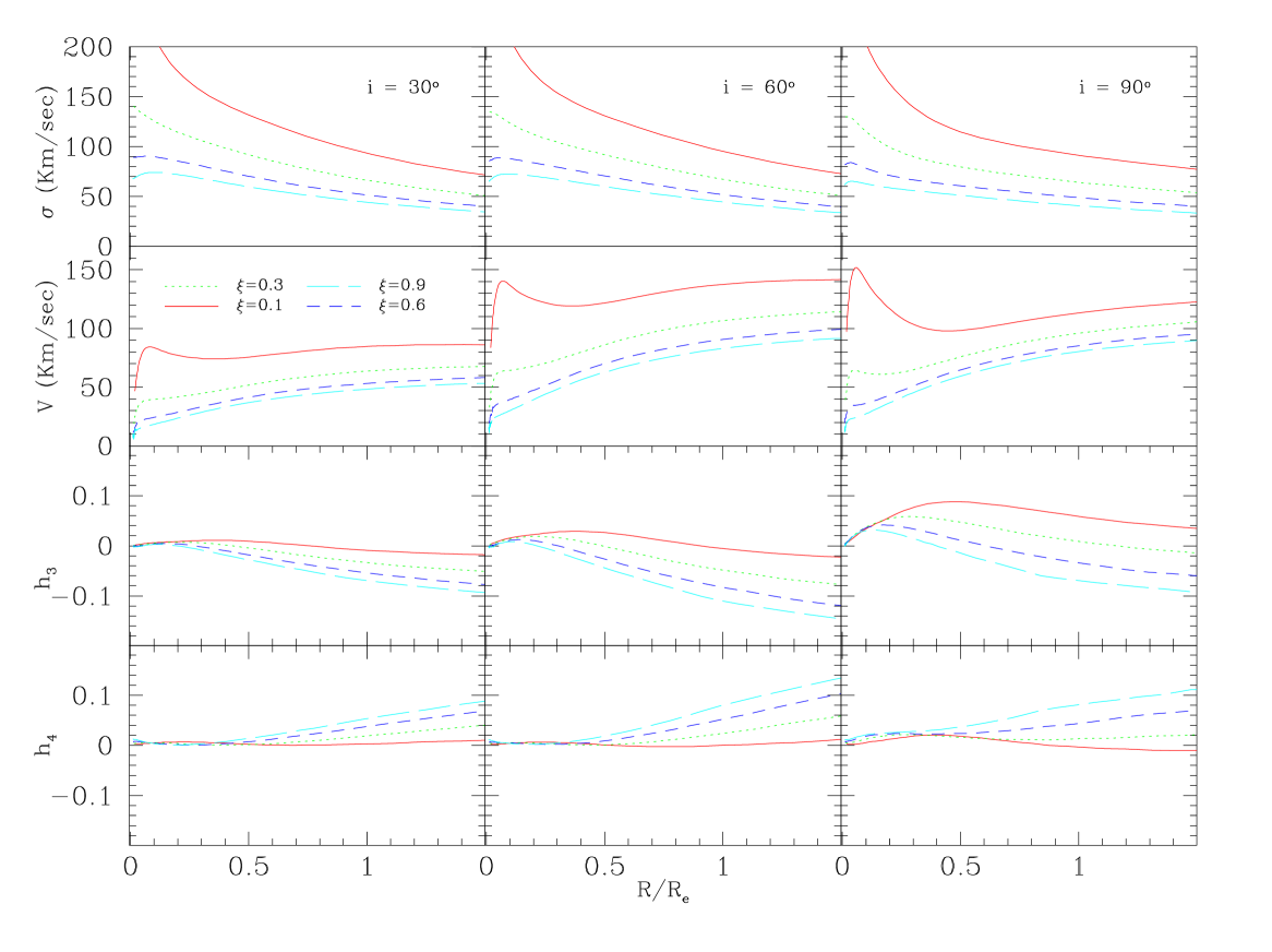
Figure 2: Rotation curves and velocity dispersion profiles for Sa galaxies, varying the concentration of the bulge relative to the disk components, and the inclination angle $i$. The two panels below also show the $h_{3}$, $h_{4}$ parameters profiles as described by the model. All the quantities are referred to a galaxy of $M=10^{11}\hbox{$\rm M_{\sun}$}$, and $R_{\rm e}=10\,\mbox{kpc}$. The scaling factor is described into the text.

The classification of galaxies in a single unificating scheme has been one of the earlier results in the study of stellar systems. The details of this classification are, however, still under discussion. Along the sequence of disk galaxies, the classification of galaxies may be expressed in terms of photometric properties, such as the relative weights of the bulge and disk component and their relative concentration. Our model allow a dynamical deduction of these properties. We can compare observed velocity- and velocity dispersion- curves with that of a model galaxy, projected at the same viewing angle of the real galaxy and integrated along the line-of-sight. In such a way, one can deduce the disk-to-bulge ratio of the galaxy in terms of mass ratio and relative concentration of the two components. We expect that this dynamical description may give different results with respect to the disk/bulge ratio photometrically deduced, and allow to correct the $M/L$ ratio assumed and eventually detect the presence of dark matter contained in the inner/intermediate portion of the galaxy.

To make this comparison easy, the dimensionless quantities $V_{\rm mod}$, $\sigma_{\rm mod}$, produced by the model should be correlated with the physical parameters. Since the model quantities are produced in the dimensionless system having $GM_{\rm tot}=1$ and $R_{\rm e,tot}=1$, they can be related to the observables by the use of the simple scaling law:

$$V_{\rm obs} = \sqrt{\frac{GM_{\rm tot}}{R_{\rm e,tot}}}\cdot V_{\rm mod}$$

$$\sigma_{\rm obs} = \sqrt{\frac{GM_{\rm tot}}{R_{\rm e,tot}}}\cdot\sigma_{\rm mod}$$

We then produced a set of rotation- and velocity dispersion curves for six type of galaxies having different bulge-to-disk mass ratio ($\eta$) and concentrations ($\xi$), and with a given $M_{\rm tot}=10^{11}\,\hbox{$\rm M_{\sun}$}$, and $R_{\rm e,tot}=10\,\mbox{kpc}$. In this simulation, all the components have an isotropic velocity dispersion. In order to limit the number of free parameters, we stick to the classical case of a $r^{1/4}$ bulge embedded in an exponential disk. The $M/L$ ratio of the bulge is assumed to be twice the corresponding value of the disk. In the next paragraph we will show the relevance of an anisotropic velocity dispersion in modifying the observed curves.

The curves were calculated for the galaxy seen edge-on ($90^{\circ}$) and at an inclination of $60^{\circ}$ and $30^{\circ}$. The choice of the $\eta$ values has been made trying to reproduce the main Hubble stages, from S0 to Sd, in agreement with the values deduced by Simien & de Vaucouleurs (1986). The whole grid of calculation is available on request in electronic form. We are able to reproduce the whole sequence assuming different slopes or different luminosity laws for the bulge and the disk but of course this profusion of data cannot be presented here.

In Fig. 2 we show the kinematic curves for the case of Sa galaxies (here simply defined as galaxies having an $\eta=0.68$). They are arranged with the curves having different $\xi$ shown in the same panel.

The relation between the observed curves with that presented in the figures is then:

$$V_{\rm obs} = \sqrt{\frac{M_{\rm tot}/[10^{11}\,\hbox{$\rm M_{\sun}$}]}{R_{\rm e,tot}/[10\,\hbox{kpc}]}}\cdot V_{\rm fig}$$

$$\sigma_{\rm obs} = \sqrt{\frac{M_{\rm tot}/[10^{11}\,\hbox{$\rm M_{\sun}$}]}{R_{\rm e,tot}/[10\,\hbox{kpc}]}}\cdot\sigma_{\rm fig}$$

with masses computed in solar mass units and radii in Kpc.

This procedure allows, within some limits, to consider the galaxy as a unique structure, with a typical bulge/disk ratio and bulge concentration. However, it fits also into the idea that it is possible to distinguish dynamically the galaxy type. This approach has been faced by Persic and Salucci (1996) on the basis of a sample of galaxies taken from the literature. Working on the superposition of nearly 1000 observed gas rotation curves grouped for Hubble type, the authors derived a circular rotation curve for every given Hubble type. However, since this work was mainly aimed at the detection of dark matter, more care is devoted to the outer part of the rotation curves; in addition, a poor statistic is available on the early-type disk galaxies S0 and Sa.

5.2 The anisotropy in bulges

The low rotational velocities found in elliptical galaxies with respect to their flattening (Bertola & Capaccioli 1977, Kormendy & Illingworth 1977) can be interpreted in terms of anisotropy in the stellar velocity distribution (Binney 1978). The same indications arose from the study of the velocity dispersion profiles (Tonry 1983). For similarity with elliptical galaxies, we can expect that some anisotropy could be present in bulge dynamics also. On the contrary, the presence of anisotropy in the disk component of the galaxies should be less relevant, due to the lower value of the velocity dispersion of disks compared with bulges or elliptical galaxies.

The study of velocity anisotropy in disk galaxies may give indications on the differences existing between bulges and ellipticals, contributing to understand the formation process of this two classes of objects. However, due to the composite nature of disk galaxies, to measure the anisotropy of the velocity distribution from the observables $(V,\sigma)$ is much more difficult than in the case of elliptical galaxies. Working on the same set of data, concerning four S0 and Sa galaxies, Kormendy & Illingworth (1982) deduced the isotropy of their bulges, while Whitmore, Rubin and Ford (1985) reached the opposite conclusion. Both authors used the $V/\sigma$ test, first proposed by Binney (1976) for Elliptical galaxies. The fact that the same data may be interpreted in such different ways clearly demonstrates the ambiguity of this test, when applied to the bulges of disk galaxies.

In a model of galaxy, the shape of the potential defines, on the galaxy plane, the shape of the rotation- and velocity dispersion- profiles. However, the ratio of the central velocity dispersion to the maximum rotational velocity is dependent both from the eccentricity $e$ and from the anisotropy parameter $\beta$: one may obtain in a model a higher $V/\sigma$ ratio increasing the eccentricity and/or decreasing the anisotropy parameter. As a reverse argument,we can deduce the galaxy potential by fitting the observed rotation curve along the apparent major axis but we cannot deduce from this curve the values of $e$ or $\beta$. To define the values of these parameters, we need more observable constraints.

One of this may arose from the photometry; in particular, from the value of the axial ratio obtained by fitting the observed isophotes. In such a case, the $\beta$ parameter can be, in principle, derived from the major axis kinematic curves ($V$ and $\sigma$) only. Such a case is however so rarely found in the literature, due to the great errors that can derive from the decomposition algorithms, that the photometric methods cannot be considered of general application (Seyfert & Scorza 1996).

A different approach may allow to deduce the ellipticity and anisotropy with a simultaneous fit of several rotation curves taken at different position angles or with offsets parallel to the major axis. This kind of data is available in the literature for an increasing number of galaxies and may be used to derive the anisotropy in their velocity distribution.The model presented here can support this kind of approach to estimate the amount of anisotropy present in an observed galaxy.

In the following, we shall discuss two points: first, how the anisotropy is involved in the stability of a galaxy; second, how much our model is able to distinguish between different anisotropies by means of the rotation- and velocity dispersion- curves.

Figure 3: Axial ratios and anisotropy of our models. Below the solid line lies the physically allowed space of parameters, in the simple case of a single homogeneous spheroid, and under our hypothesis of constant anisotropy. The maximum $\beta$ allowed for different values of the axial ratio in the more realistic case of two-components galaxies are shown as starred points. The labels show the location of the models described in Fig. 4.

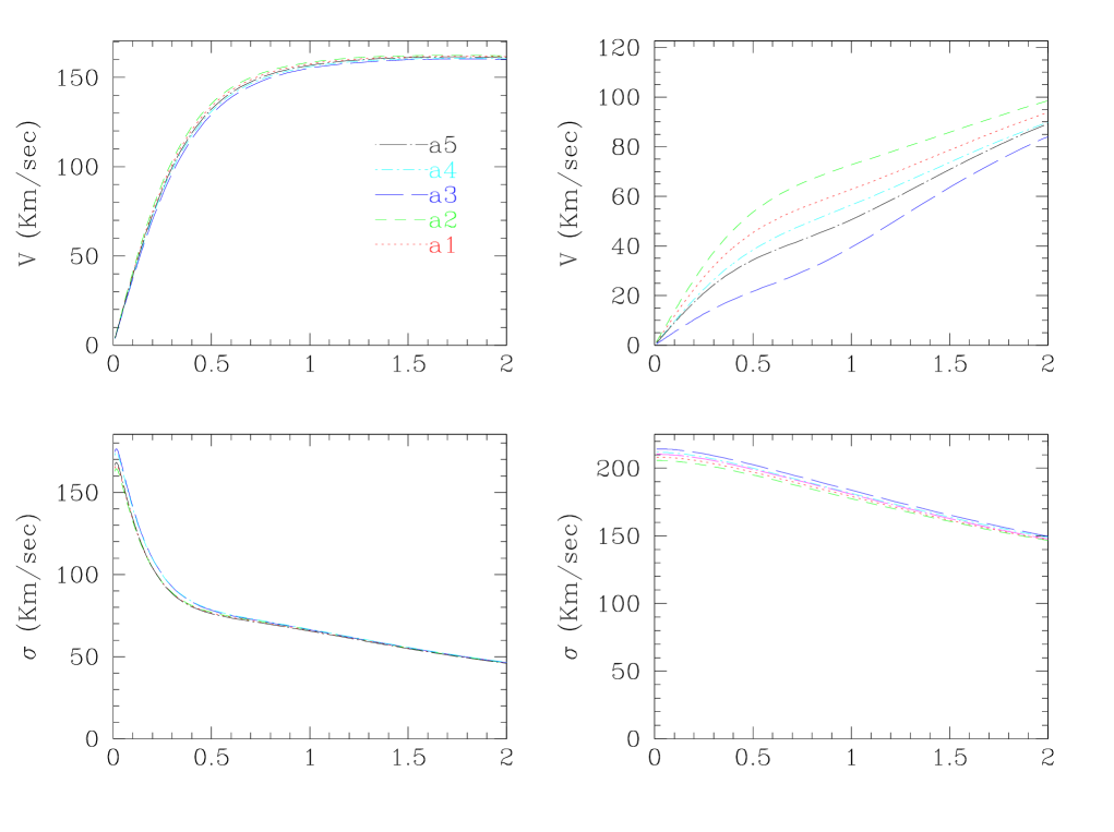
Figure 4: An example of different kinematic curves along the major axis (left panels) and along an offset parallel to the major axis but shifted by $0.5\,R_{e}$. The different curves correspond to an S0 galaxy with fixed $\xi,\eta$ values but different $(\beta,e)$. The label of the different curves refers to the pairs of $(\beta,e)$ plotted in Fig. 3.

5.2.1 Anisotropy and stability

An instability mechanism may be generated by the local excess of kinetic energy going in disordered motions with respect to the local gravitational potential. Its genesis is the following:

Under the hypothesis that the only ordered motion in a galaxy be the rotation around the $z$ axis, the $z$ component of the gravitation force can only be equilibred by the $z$ component of the velocity dispersion $\sigma_{zz}$, which is univocally determined by the distribution of matter and is not dependent from the anisotropy parameter $\beta$ . In such a galaxy, the radial component of the velocity dispersion is higher as the anisotropy increases, enhancing the importance of the asymmetric drift. As $\beta$ approaches unity, the value of $\sigma_{RR}$ tends to infinity, and so the asymmetric drift. Following this trend, the asymmetric drift correction to the dynamical equation may overcome the gravitational term of equation (6), pulling the galaxy outward and destroying the dynamical equilibrium. As a consequence, once fixed in a galaxy the axial ratio of the two components, not every values of $\beta$ are allowed. The “physical” range of this parameter is restricted to $0\leq\beta\leq\beta_{\rm max}(e)$, with $\beta_{\rm max}(e)$ derived by imposing:

$$\Delta V^{2}_{\rm asymdrift}<V_{\rm c}^{2}$$ (11)

in every point of the galaxy.

Since the circular velocity is not dependent from the anisotropy while the correction for asymmetric drift is related to it only by means of a scale factor, Eq. (11) can be rewritten as

$$f(e)\equiv\frac{\Delta V^{2}}{V^{2}_{\rm c}}(\beta=0)<1-\beta$$ (12)

so that the dependence from the $\beta$ parameter is easy to handle.

The $f(e)$ can be computed analytically in the limit case of homogeneous spheroids only; the result is shown in Fig. 3 with a solid line. In the realistic case, with two-components and peaked density profiles, $f(e)$ must be computed numerically. We estimated the limiting $\beta_{\rm max}$ from a set of models with bulges of different ellipticities. The results are shown in Fig. 3 (starred symbols), showing that the homogeneous spheroids curve can be used as a starting point for the analysis of the realistic cases.

Again, we must point out here that this limiting values of $\beta$ are only valid under our hypothesis of $\sigma_{RR}==\sigma{\phi\phi}$, and should certainly be recalculated in different kinematic conditions.

Table 1: Parameters from the Dynamical Model for NGC 5866. The labels $b$ and $d$ refers to the bulge and disk components.

scale radius

axial ratio

Luminosity

Mass [10${}^{10}M_{\odot}$]

rb

rd

(b/a)b

(b/a)d

Lb

Ld

Mb

Md

i

$35\prime\prime$

$15\prime\prime$

0.8

0.15

62 %

38 %

5.58

1.72

$71^{\circ}$

5.2.2 Inferring the anisotropy from observations.

An observer may estimate the anisotropy present in a galaxy only if the difference between models with different anisotropy are greater than the observational errors. In order to give a rough estimate of the diagnostic power of the model in determining the anisotropy parameter $\beta$, we produced several models in different regions of the diagram of Fig. 3. Looking at the literature, a conservative estimate for the observational errors in kinematic curves may be established assuming $\Delta V=20$ km/sec and $\Delta\sigma$ = 40 Km/s.

Curves of a typical model with different anisotropy and bulge flattening are shown in Fig. 4. Looking at this figure, one can see that the difference in velocities generated by a change of anisotropy of 0.1 produces a negligible variation along the apparent galaxy major axis. On the contrary, significant variations are observable along offset axes, e.g. setting the slit parallel to the major axis but shifted by 0.5 $R_{e}$, as shown in the same figure. The highest differences are visible in the rotation curve (as great as 40 km s^-1) while the velocity dispersion curves are less sensitive ($\leq 10\mbox{ km\,s${}^{-1}$}$).

The sensitivity of the projected kinematic curves to variations of $\beta$ or $e$ is different for galaxies lying in different regions of the $(\beta,e)$ plane. We can distinguish three typical cases:

1. Almost spherical bulges Under our assumption of homogeneous anisotropy, an almost spherical model (with bulge having $b/a>0.85$ ) does not allow stable solutions with significant anisotropy.

2. Strongly flattened bulges This is the opposite situation ($b/a<0.4$). In this case, the diagnostic power of the model in determining anisotropy is limited. The offset curves give only poor additional information with respect to that obtained from the major axis data. In real galaxies this mean flattening is observed only in the late-type spirals, where the disc is preponderant with respect to the spheroidal component. As a consequence, the bulge gives a low contribution to the global kinematics.

3. Intermediate models The higher efficiency of the models in distinguishing the anisotropy of a real galaxy from observations is found for galaxies with bulges having intermediate flattening ($0.4\leq b/a\leq 0.85$). The offset rotation curve is very sensitive to the $\beta$ parameter changes, as described above in the example of Fig. 4. The presence of an offset spectrum may delete, in this case, the uncertainties on the value of $\beta$ derived from observations along the major axis.

6 A test case: NGC 5866

We tested our model using a real case of a galaxy for which a complete set of photometric and kinematic data exists in the literature. We chose NGC 5866, for which rotational velocity and velocity dispersion profiles are available along the major axis and at different offsets from the nucleus (Kormendy & Illingworth 1982). This galaxy is an S0 seen almost edge-on, showing a prominent dust lane on the major axis, clearly visible in Fig. 5 and in the photometric profiles (Fig. 6).

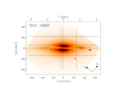
Figure 5: An image of the galaxy NGC 5866. The approximate position and extension of the kinematic profiles (Fisher 1997, Kormendy & Illingworth 1982) are shown superimposed on the multi-color image of the galaxy (Peletier and Balcell 1997).

Figure 6: Major and minor axis R-band photometric profiles, compared with the two components best-fit model. The dashed lines shown the contribution of the bulge and disk to the total surface brightness profiles (solid line). The crossed circle represent the points which have been excluded from the automatic fit due to the effect of the absorption of the dust lane.

We took the recent kinematic data published by Fisher (1997) as well as that published by Kormendy and Illingworth (1982).We adopted the photometry made by Peletier and Balcell (1997). The full set of data to be reproduced by our model include the profiles of velocity dispersion and rotational velocity taken along 7 different axis across the galaxy. The position of the axis where kinematic data are available are shown in Fig. 5. The $h_{3}$ and $h_{4}$ parameters are also published but not for all the positions of the slit.

The effect of the dust is marked in the innermost 5 arcsec along the major axis. For this reason we neglected the regions more heavily obscured by the dust from our photometric fit (see Fig. 6), relaxing the fit along the major axis luminosity profile, where the dust absorption is more effective.

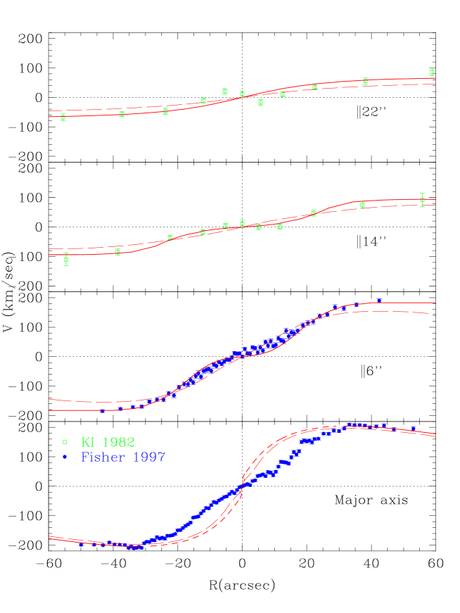
Figure 7: Rotational velocity profile of stars and gas as compared to the model of the stellar kinematics, for the axis parallel to the major axis. The dashed line on the model correspond to the region obscured by the dust lane. In this plot we also show for comparison the best results for an anisotropic model with $\beta=0.1$ (long-dashed line).

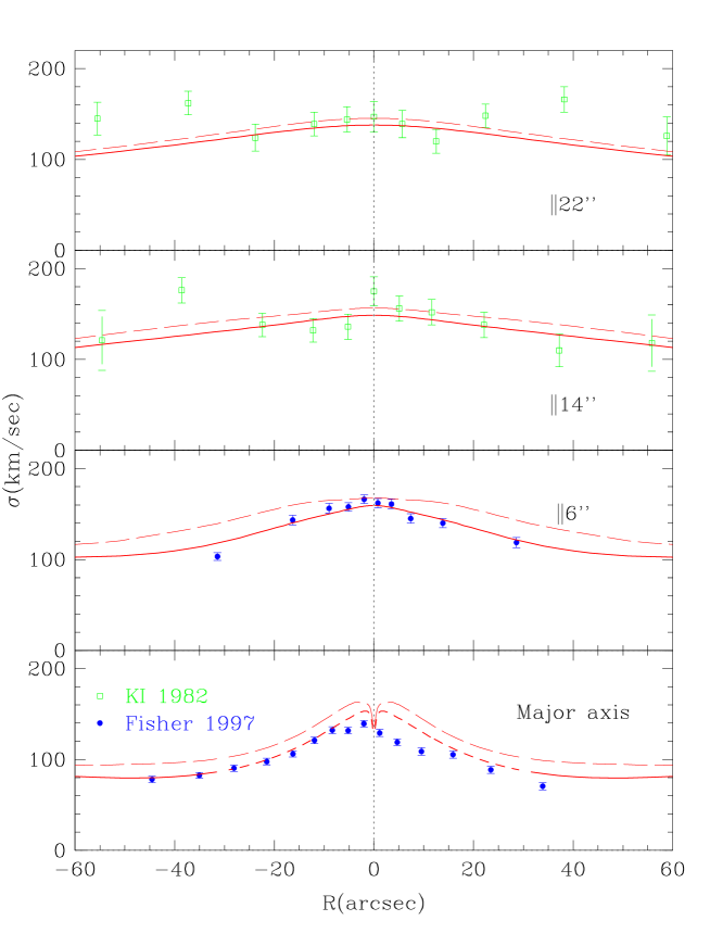
Figure 8: Same as Fig. 7, but for the velocity dispersion profiles. Note the bad performance of the anisotropic model.

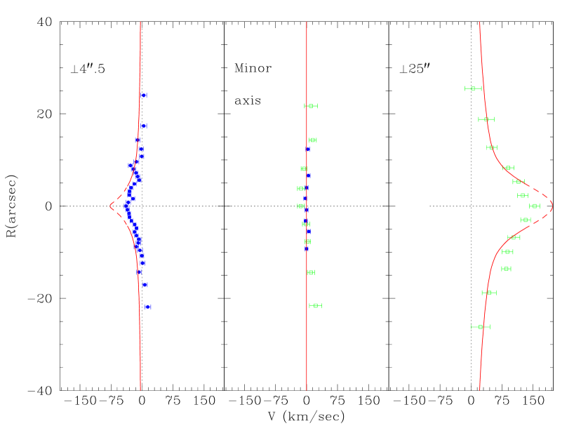
Figure 9: Same as in Fig. 7, but for the perpendicular cut shown in Fig. 5. We avoided to display the anisotropic model here.

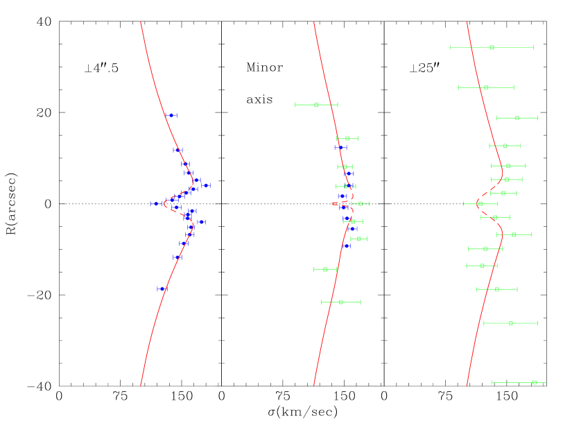
Figure 10: Same as in Fig. 8, but for the perpendicular cut shown in Fig. 5.

The best-fit we adopted arise from a two-component (bulge+disk) model whose parameters are shown in Tab. 1. With these values, we computed by means of our model the expected, self-consistent kinematics of this galaxy. According to our expectations, the results reproduce most of the observed feature of the kinematics:

• In general, the trend of the rotation curves and of the velocity dispersion profiles agrees everywhere with the model, except in the regions obscured by the dust (see Fig. 7). The explanation of this effect may be understood if the optical thickness is high. In such a case, we only observe the stars on the outer edge of the disk, whose line-of-sight velocity components are very low.

• On the other hand, the presence of the dust is only slightly affecting the velocity dispersion, as expected in a dynamically hot system such as an early-type galaxy. Our profiles agree with the observations even in the regions obscured by dust. Along the major axis the velocity dispersion profile is monotonically decreasing from a peak value of 140 km s^-1in the central region to $\sigma\approx 74$ km s^-1at $40^{\prime\prime}$. On the major-axis offset positions, slightly higher velocity dispersion are observed. The minor-axis data indicate that the velocity dispersion rises marginally with increasing $z$ height (from $\approx 150$ km s${}^{-}1$ to $\approx 158$ km s^-1at $6^{\prime\prime}$) and decrease at larger radius. The same behavior is present in the minor-axis offset spectra. Fisher (1997) proposed that this is an observational effect due to the dust obscuration: our model seem to indicate that this is indeed a real effect, due to the dominance of the cold disk component at $z\approx 0$.

• Along the major axis, far from the region heavily obscured by the dust, the model rotation curves flattens according to the observed data. Fitting the observed maximum rotational velocity of 203 km s^-1, we find a total mass for the galaxy of $(7.3\pm 0.5)\cdot 10^{10}$ $\rm M_{\sun}$. Fairly rapid rotation is seen even at heights of several kpc above the disk plane. At $z=6^{\prime\prime},r=40^{\prime\prime}$ the offset spectrum has a speed of 184 km s^-1. At $z=22^{\prime\prime}$, equivalent to an height of 2 kpc above the disc plane, the rotation curve reaches $\sim$100 km s^-1, a value comparable with the mean dispersion $\sigma\approx 150$ km s^-1observed in the bulge. This is compatible with the isotropic model we are proposing, while no model with significant amount of anisotropy has been found to be able to improve the fit of the data.

• No rotation is seen along the minor axis ($V_{min}=3\pm 3$ km/sec), so we can likely exclude misalignments between the different components or a significant bulge triaxiality.

• The fit of the $h_{3}$ and $h_{4}$ parameters are marginally satisfactory on the major axis, taking into account the effects of the dust; but are poorer on the offset at $6^{\prime\prime}$. However, having considered the deviations from the pure Gaussian shape of the line profile greatly improved the quality of the $V,\sigma$ fit.

7 Conclusions

Our self-consistent, two-components model of disc galaxy may reproduce the photometric and the kinematic properties of the disc galaxies of different morphological type. In particular:

1. The model is able to produce rotation curves, velocity dispersion profiles and h₃, h₄ curves for disc galaxies from S0 to Sd, describing the different models in terms of relative weight and the concentration of the bulge with respect to the disc. A library of model curves, projected at different angles of galaxy inclination with respect to the sky plane has been generated. The comparison of these models with observations of real galaxies needs only two scaling factors: the total mass and the effective radius.

2. The anisotropy of the velocity field has been studied as instability generator inside the galaxy. We showed that for each given value of the bulge axial ratio a stable stellar system cannot possess a value of anisotropy greater than a fixed value. In the extreme case of spherical systems, only isotropic distributions of velocities are allowed, under our assumption of anisotropy homogeneous across the galaxy.

3. The models show a strong diagnostic power in detecting anisotropy in the bulges of the early-type disc galaxies when spectra outside of the apparent major axis are available. The best results are obtainable in the case of bulges of intermediate ($0.4\leq b/a\leq 0.85$) flattening, close to the values observed in real galaxies. In this case, an anisotropy change of 15% may give variations even of 40-50% in the offset rotation curves, as shown in Fig. 4.

4. The application of the model to edge-on S0 galaxy NGC 5866 has been presented. It suggests an isotropic distribution of velocity and is able to reproduce the global galaxy kinematics ($V$ and $\sigma$ profiles).

Acknowledgments

This work has been partially supported by the grant “Astrofisica e Fisica Cosmica” Fondi 40% of the Italian Ministry of University and Scientific and Technologic Research (MURST).

Appendix A. Gauss-Hermite expansion of the line shape.

One should address the question how the deviations from the pure Gaussian profile are best quantified.

Van der Marel & Franx (1993) represented the line profile as a sum of orthogonal functions in a Gauss-Hermite series. The expansion naturally leads to two parameters describing deviations from a Gaussian: a parameter $h_{3}$ describing asymmetric deviations, and a parameter $h_{4}$ describing symmetric deviations.

The LOSVDs $f(v)$ can then be described by a Gaussian plus third- and fourth-order Gauss-Hermite functions:

$$f(v)=I_{0}\exp(-y^{2}/2)(1+h_{3}{\cal H}_{3}(y)+h_{4}{\cal H}_{4}(y))$$ (A1)

with $y=(v-v_{fit})/\sigma_{fit}$, and where

$${\cal H}_{3}(y)=(2\sqrt{2}y^{3}-3\sqrt{2}y)/\sqrt{6}$$ (A2)

$${\cal H}_{4}(y)=(4y^{4}-12y^{2}+3)/\sqrt{24}$$ (A3)

are the standard Gauss-Hermite polynomials, $u_{i}=exp(-y^{2}/2)\times{\cal H}_{i}(y)$ are the Gauss-Hermite basis functions, and $h_{3}$ and $h_{4}$ are their amplitudes. $I_{0}$ is a normalization constant.

References

- [Bertola et al. 1984] Bertola, F., Bettoni, D., Rusconi, L., Sedmak, G. 1984, AJ 89, 356
- [Bertola & Capaccioli 1975] Bertola, F., & Capaccioli, M., 1975 ApJ 200, 439
- [Bertola & Capaccioli 1977] Bertola, F., & Capaccioli, M., 1977 ApJ 211, 697
- [Bertola et al. 1991] Bertola, F., Vietri, M., Zeilinger, W.W., 1991, ApJ, 374, L13
- [Binney 1976] Binney, J. J. 1976, MNRAS. 177,19
- [Binney & De Vaucouleurs 1981] Binney, J. and De Vaucouleurs, G., 1991, MNRAS 194, 679
- [Binney et al. 1990] Binney, J. J., Davies, R. L., Illingworth, G. 1990, ApJ 361,78
- [Binney & Tremaine 1987] Binney, J. & Tremaine, S., 1987, Galactic Dynamics, Princeton University Press
- [Ciotti 1991] Ciotti, L., 1991, A&A 249, 99
- [Cretton & van den Bosch 1999] Cretton, N., van den Bosch, F. C., 1999, ApJ 514, 704
- [Dehnen & Gehrard 1993] Dehnen, W., Gerhard, W.D., 1993, MNRAS 261,311
- [Emsellem et al. 1994] Emsellem, E., Monnet G., Bacon, R., A&A 285, 723
- [Emsellem et al. 1999] Emsellem, E., Dejonghe, H., Bacon, R., 1999, MNRAS 303, 495
- [Fillmore et al. 1986] Fillmore, J.A., Boroson, T.A., Dressler, A., 1986, ApJ, 302, 208
- [Fisher 1997] Fisher, D., 1987, AJ 113, 950
- [Grosböl 1985] Grosböl, P. J., 1985, A&AS 60, 261
- [Kormendy 1984] Kormendy, J., 1984, ApJ, 286, 116
- [Kormendy & Illingworth 1982] Kormendy, J. & Illingworth, G., 1982, ApJ 256, 460
- [Kuijken & Merrifield 1993] Kuijken, K. and Merrifield, M. R. 1993, MNRAS 264, 712
- [Illingworth & Schechter 1982] Illingworth , G., & Schechter, P.L., 1982, ApJ, 256, 481
- [Loyer et al. 1998] Loyer, E., Simien, F., Michard, R., Prugniel, P., 1998, A&A 334, 805
- [Magrelli et al. 1992] Magrelli, G., Bettoni, D., Galletta, G. MNRAS 1992, 256, 500
- [Merritt 1999] erritt, D., 1999, PASP 111, 129
- [Monnet & Simien] G. Monnet and F. Simien, 1977, A&A 56, 173
- [Peletier & Balcells 1997] Peletier, R. F. & Balcells, M., 1997, New Astronomy 1, 349
- [Persic & Salucci 1996] Persic, M. , Salucci, P. & Stel, F., 1996, MNRAS 283, 1102
- [Prugnel & Simien 1997] Prugniel, P. & Simien, F., 1997, A&A 321, 111
- [Pignatelli 1996] Pignatelli, E., 1996, PhD thesis, University of Padova
- [Rix et al. 1997] Rix, H.-W., de Zeeuw, P.T., Cretton, N., van der Marel, R.P., Carollo, C.M. 1997, ApJ 488, 702
- [Sandage et al. 1970] Sandage, A., Freeman, K. and Stokes, N.R., 1970, ApJ 160, 831
- [Sargent et al. 1977] Sargent, W.L.W., Schechter, P.L., Boksenberg, A. and Shortridge, K. 1977, ApJ 212,326
- [Satoh 1980] Satoh, C., 1980, PASJ 32, 41
- [Schwarzschild 1979] Schwarzschild, M., 1979, ApJ 232, 236
- [Simien & De Vaucouleurs 1986] Simien, F. & De Vaucouleurs G., 1986, ApJ 302, 564
- [Seifert & Scorza 1996] Seifert, W., and Scorza, C., 1996, A&A 310, 75
- [Stark 1977] Stark, A. A. 1977, ApJ 213, 368
- [Tonry 1983] Tonry, J.L., 1983, ApJ, 266,58
- [van der Marel & Franx, 1993] van der Marel and Franx, 1993, ApJ 407, 525B
- [Young 1976] Young,P.J., 1976, AJ, 81, 807
- [van der Hulst 1961] van der Hulst, C.J., 1961 B.A.N., 509, 1
- [van der Marel et al. 1998] van der Marel, R.P., Cretton, N., de Zeeuw, P.T., Rix, H.-W., 1998, ApJ 493, 613
- [Whitmore et al. 1985] Whitmore, B.C., Rubin, V.C., Ford, W.K., 1985, ApJ 287, 66
- [Zeilinger et al. 1990] Zeilinger W.W., Galletta, G., Madsen, C., 1990, MNRAS, 246, 324