Validity of the ‘Conservation Law’ in the Evolution of Cosmological Perturbations

Abstract

It is shown that the ‘conservation law’ for metric fluctuations with long wavelengths is indeed applicable for growing modes of perturbations, which are of interest in cosmology, in spite of a recent criticism [1996]. This is demonstrated both by general arguments, and also by presenting an explicitly solvable toy model for the evolution of metric perturbations during inflation.

1 Introduction

The gauge-invariant theory of cosmological perturbations (see Mukhanov, Feldman & Brandenberger [1992] for a review) has been used successfully to calculate the origin and evolution of metric and density perturbations in the early universe. The most beautiful aspect of this approach is that the evolution of metric perturbations with wavelengths larger than the Hubble radius, where the growth in amplitude during inflation takes places, is characterized by a simple conservation law

$$\zeta=\frac{2}{3}\frac{\dot{\Phi}/H+\Phi}{1+w}+\Phi=\mathrm{const.},$$ (1)

where $\Phi$ denotes the gauge-invariant generalized Newtonian potential for scalar metric perturbations, $w=p/\epsilon$ the equation of state of the matter content, and $H$ the Hubble parameter (Equ. (5.23) and (6.58) in Mukhanov et al. [1992]). It should be noted though that this is valid only for perturbations in a universe with a spatially flat background metric (i.e. $K=0$), which was not stated after Equ. (5.23) in Mukhanov et al. [1992]. Therefore only the case $K=0$ will be considered in this paper.

The growth of fluctuations in a universe with a de Sitter-phase is apparent from (1), since $w\sim-1$ during inflation leads to a small denominator for $\zeta$ such that the amplitude of $\Phi$ has to increase considerably in order to keep $\zeta$ constant as the universe exits inflation into a radiation ($w=1/3$) or matter dominated phase ($w=0$).

Recently, there has been a criticism by Grishchuk [1996] that the conservation of $\zeta$ is derived from an incorrect equation of motion for the cosmological perturbations and that it is always zero in the limit of long wavelengths, in which case no statement on the evolution of scalar metric perturbations would be possible, as $\Phi$ could be multiplied by any arbitrary factor without affecting the value of $\zeta$.

In this paper we will show that the equation used in deriving that $\zeta$ is constant in the long-wavelength limit is indeed the correct one, and that furthermore $\zeta$ always takes non-zero values for growing modes and can become zero only for decaying ones. This will be exemplified by explicitly constructing a toy model for which the evolution of metric perturbations during inflation can be determined analytically. This is different from previously proposed toy models for that purpose [1996] in which the equation for the metric perturbations had to be integrated numerically. Hence we show that the conservation law (1) is indeed a useful relation to describe the evolution of metric perturbations at large wavelengths. Note that earlier criticism by Grishchuk [1994] has been refuted by Deruelle & Mukhanov [1995] and by Caldwell [1996].

2 General Remarks

The basic equation governing the time dependence of the metric fluctuations $\Phi$ (Equ. (5.22) and (6.49) in Mukhanov et al. [1992]) is a linear combination of the time-time and space-space components of the linearized Einstein perturbation equations expressed in terms of gauge-invariant variables. For the case of a universe with a single scalar field ($\phi$ is its unperturbed background value) this equation reads

$$\Phi^{\prime\prime}+2\left(\frac{a}{\phi^{\prime}}\right)^{\prime}\frac{\phi^{\prime}}{a}\Phi^{\prime}+\mn@boldsymbol{k}^{2}\Phi+2\phi^{\prime}\left(\frac{\mathcal{H}}{\phi^{\prime}}\right)^{\prime}\Phi=0$$ (2)

for a Fourier mode with wavenumber $\mn@boldsymbol{k}$, where primes denote differentiation with respect to conformal time, $a$ the scale factor, and ${\mathcal{H}}=a^{\prime}/a$. The conservation law (1) follows from this with some simple algebra.

Alternatively, fluctuations can be described by a linear combination of the metric perturbations $\Phi$ and the gauge-invariant scalar field perturbations $\delta\phi$

$$v=a\left(\delta\phi+\frac{\phi^{\prime}}{\mathcal{H}}\Phi\right)$$

(Equ. (10.71) in Mukhanov et al. [1992]; $v$ is called $\mu$ and $\nu$ in Grishchuk [1996]) which arises in the derivation of the Lagrangian for the Einstein perturbation equations. Varying the corresponding action gives the equation of motion

$$v^{\prime\prime}+\mn@boldsymbol{k}^{2}v-\frac{z^{\prime\prime}}{z}v=0$$ (3)

for that variable, where $z=a\phi^{\prime}/{\mathcal{H}}$. By taking advantage of the equation for the evolution of the scalar field background and the constraint equation for $\Phi$, the relation between the two gauge-invariant variables $\Phi$ and $v$ can be brought in the form

$$-\mn@boldsymbol{k}^{2}\Phi=4\pi G\frac{\phi^{\prime 2}}{\mathcal{H}}\left(\frac{v}{z}\right)^{\prime}$$ (4)

(Equ. (13.7) in Mukhanov et al. [1992]) with Newton’s constant $G$.

We expect that both Equ. (2) and Equ. (3) should yield the same physical results for the evolution of cosmological perturbations, i.e. it should be possible to go back and forth between these two different ways to formulate the problem. But as we substitute relation (4) between the two gauge-invariant variables in (2) in an attempt to recover (3) we actually end up with

$$\left(v^{\prime\prime}+\mn@boldsymbol{k}^{2}v-\frac{z^{\prime\prime}}{z}v\right)^{\prime}-\frac{z^{\prime}}{z}\left(v^{\prime\prime}+\mn@boldsymbol{k}^{2}v-\frac{z^{\prime\prime}}{z}v\right)=0,$$ (5)

an equation which admits more solutions than (3), from which Grishchuk [1996] argues that the equation for the metric perturbations $\Phi$ is the wrong one to begin with.

Here I would like to argue that (2) and (3) are still equivalent. The problem is that in order to substitute (4) we have to multiply the equation for $\Phi$ by $\mn@boldsymbol{k}^{2}$ (or $\nabla^{2}$ in position space), thus it is no surprise that we find more solutions than we need. For that reason (5) is not equivalent to (2), but to another equation

$$\Phi^{\prime\prime}+2\left(\frac{a}{\phi^{\prime}}\right)^{\prime}\frac{\phi^{\prime}}{a}\Phi^{\prime}+\mn@boldsymbol{k}^{2}\Phi+2\phi^{\prime}\left(\frac{\mathcal{H}}{\phi^{\prime}}\right)^{\prime}\Phi=f(\mn@boldsymbol{k})$$ (6)

where the right-hand side is replaced by an arbitrary, possibly time-dependent function subject only to the condition $\mn@boldsymbol{k}^{2}f(\mn@boldsymbol{k})=0$, e.g. a $\delta$-function. So we need to check for each of the three basic solutions of (5) whether their corresponding $\Phi$-modes give a zero or non-zero result on the right-hand side of (6) and disregard the latter ones.

It is easy to determine that the full set of solutions of (5) is

$$v(\mn@boldsymbol{k},\eta)=C_{1}v_{1}(\mn@boldsymbol{k},\eta)+C_{2}v_{2}(\mn@boldsymbol{k},\eta)+C_{3}\frac{z}{\mn@boldsymbol{k}^{2}}$$

where $v_{1}$ and $v_{2}$ are the two linearly independent solutions of the original equation (3) for $v$ and $\eta$ denotes conformal time. Exploiting that $v_{1}$ and $v_{2}$ satisfy (3) we can rewrite the relation between $\Phi$ and $v$ as

$$\Phi_{i}=\frac{4\pi G{\mathcal{H}}}{a^{2}}\int v_{i}z\,{\mathrm{d}}\eta+h(\mn@boldsymbol{k}),\;i=1,2$$ (7)

where $h(\mn@boldsymbol{k})$ is another arbitrary, potentially time-dependent function satisfying $\mn@boldsymbol{k}^{2}h(\mn@boldsymbol{k})=0$. Using this relation in (6) we see that these two modes for $\Phi$ do indeed give zero on the right-hand side as long as $h(0)$ is zero or itself a solution of the original equation (2) for $\Phi$ for $\mn@boldsymbol{k}=0$, which means it has to be a linear combination of $\Phi_{1}$ and $\Phi_{2}$ in that case. (For $\mn@boldsymbol{k}\neq 0$ we already have $h(\mn@boldsymbol{k})=0$.) Since it does not matter which linear combination we call the basic solutions we can set $h(\mn@boldsymbol{k})=0$ in (7) without loss of generality. For the third mode $z/\mn@boldsymbol{k}^{2}$ of $v$ we have to use the original relation (4) to obtain a third mode $\Phi_{3}=h(\mn@boldsymbol{k})$ for $\Phi$, where again we have some function with $\mn@boldsymbol{k}^{2}h(\mn@boldsymbol{k})=0$. This mode will, in general, produce a non-zero result on the right-hand side of (6), unless, like before, it is a linear combination of the other two modes for $\mn@boldsymbol{k}=0$ when $h(\mn@boldsymbol{k})$ might be non-zero, in which case it will not give any new information.

Thus it makes no difference whether we describe cosmological perturbations in terms of metric perturbations $\Phi$ alone, or with the combined gauge-invariant variable $v$, as we can map the solutions of (2) and (3) into each other with relation (7) (and $h(\mn@boldsymbol{k})=0$). If we use this, we find after some algebra that the conserved quantity in terms of $v$ is simply

$$\zeta=\frac{v}{z},$$ (8)

a result which is valid for any wavenumber $\mn@boldsymbol{k}$. As for long wavelengths $v=z$ is one obvious solution to (3) we see immediately that there exist modes for which $\zeta$ is constant and non-zero in that limit. The problem with the argument for $\zeta=0$ in Grishchuk [1996] is that the limit $\mn@boldsymbol{k}\rightarrow 0$ is not taken consistently, otherwise the author would have recovered (8) instead of $\zeta=0$ (see Caldwell [1996] and Salopek [1996]).

By looking at the definition (1) of $\zeta$ we can strengthen the previous result by showing that it must take non-zero values for growing modes of the perturbations. For such modes $\left|\Phi\right|$ has to increase with time since $\Phi$ characterizes the deviation from the unperturbed background metric. That means that we must have $\dot{\Phi}>0$ for $\Phi>0$ or $\dot{\Phi}<0$ for $\Phi<0$, at least for some interval of time. Furthermore, the equation of state starts out with $w$ close to $-1$ and then increases with time in realistic models of inflation, such that $1+w\geq 0$. Since the Hubble parameter is always positive, we see immediately from (1) that $\zeta$ must take a non-zero value during the time interval in question. But by its constancy in the long-wavelength limit this means that $\zeta\neq 0$ for all times for growing modes of metric perturbations. The only chance for $\zeta$ to become zero is for decaying modes where $\left|\Phi\right|$ decreases and $\Phi$ and $\dot{\Phi}$ have opposite signs. But their contribution to the evolution of fluctuations is negligible.

The situation when the equation of state is constant, e.g. after inflation ended, requires a separate discussion, since a growing mode does not exist in this case. Indeed, for $w=\mathrm{const.}$ the differential equation for metric fluctuations in a spatially flat universe has the general solution

$$\Phi=c_{1}+c_{2}\exp\left(-\frac{5+3w}{2}\int H\,{\mathrm{d}}t\right),$$

where $c_{1}$ and $c_{2}$ are arbitrary constants, such that the dominant mode is constant instead of growing. (The fastest way to actually derive this solution is to use the conservation law (1).) But the conserved quantity becomes now

$$\zeta=c_{1}\left(1+\frac{2}{3}\frac{1}{1+w}\right),$$

hence $\zeta$ is still non-zero if the dominant mode is present (i.e. if $c_{1}\neq 0$).

A simple, exactly solvable toy model will further exemplify the case with inflation and varying $w$.

3 The Toy Model

In the toy model, we use chaotic inflation with a simple, real scalar field $\phi$ in a spatially flat universe with zero cosmological constant. The potential is a double well of the form

$$V(\phi)=b^{2}\left[\left(\frac{3l}{4}\right)^{2}\phi^{4}-\frac{1}{2}\phi^{2}\right]$$ (9)

with $l^{2}=8\pi G/3$ and $b>0$ an arbitrary parameter (see Fig. 1).

Figure 1: The double well potential (9) plotted in rescaled units as $l^{2}V/b^{2}$ versus $l\phi$. Initial conditions for the scalar field are such that it asymptotically approaches the central maximum as $t\rightarrow\infty$.

The time evolution of the scalar field during inflation with this potential can not be solved for explicitly, unless we impose the special initial conditions

$$\phi(t_{\mathrm{i}})=\phi_{\mathrm{i}},\;\dot{\phi}(t_{\mathrm{i}})=\dot{\phi}_{\mathrm{i}}\stackrel{{\scriptstyle\textstyle!}}{{=}}-b\phi_{\mathrm{i}}$$ (10)

at the beginning of inflation. Then we find (e.g. with Equ. (6.9) and (6.10) in Mukhanov et al. [1992])

$$\phi(t)=\phi_{\mathrm{i}}{\mathrm{e}}^{-b\left(t-t_{\mathrm{i}}\right)}$$

and for the Hubble parameter

$$H=\frac{3bl^{2}{\phi_{\mathrm{i}}}^{2}}{4}{\mathrm{e}}^{-2b\left(t-t_{\mathrm{i}}\right)},$$ (11)

both simple exponential decays.

It should be pointed out that initial conditions (10) involve serious fine-tuning as we give the scalar field just enough kinetic energy to asymptotically roll up the central maximum of the potential. In this toy model, the potential will not end up in one of the minima of the potential.

The equation of state evolves as

$$w={\left(\frac{4}{3l\phi_{\mathrm{i}}}\right)}^{2}{\mathrm{e}}^{2b\left(t-t_{\mathrm{i}}\right)}-1,$$

so in order to get a sufficient amount of inflation at early times we have to require

$${\left(\frac{3l\phi_{\mathrm{i}}}{4}\right)}^{2}\gg 1.$$ (12)

Using the Hubble parameter (11) we see that this condition is equivalent to $1/b\gg 1/H$ for times close to $t_{\mathrm{i}}$, i.e. the time scale of change of the scalar field is much larger than the Hubble time. Thus (12) is just a slow rolling condition for the initial evolution of the scalar field.

Note though that in this scenario $w$ does not approach a finite value, like $0$ or $1/3$, but keeps growing indefinitely. This is caused by both the pressure and energy density of the scalar field approaching zero at late times, but in such a way that their ratio tends to infinity. In a realistic model of inflation we should also consider the presence of matter and/or radiation which will dominate pressure and energy density at late times when the contribution from the scalar field has fallen off to low values, with $w$ approaching the level typical for matter and/or radiation. Hence the indefinite growth of the equation of state in this model just indicates that it is useful only up to a certain time. The slow rolling condition (12) ensures that the model is applicable long enough to get a sufficient amount of inflation.

4 Metric Perturbations in the Toy Model

The time evolution of the gauge-invariant generalized Newtonian potential $\Phi$, which characterizes scalar metric perturbations, is governed by Equ. (2). It is hard to solve in general, but proper substitutions reduce this differential equation to a confluent hypergeometric one in our case. That way, two linearly independent base solutions in the long-wavelength limit are found as (using the relations and series expansions for confluent hypergeometric functions from Section (13.1) in Abramowitz & Stegun [1965])

$$\Phi=\tau{\mathrm{e}}^{\tau}$$ (13)

and

$$\Phi=1+\tau\left[{\mathrm{e}}^{\tau}\left(\gamma+\ln\tau\right)-\sum_{k=1}^{\infty}\frac{\tau^{k}}{k!}\sum_{\nu=1}^{k}\frac{1}{\nu}\right]$$ (14)

with the abbreviation

$$\tau=\frac{3l^{2}{\phi_{\mathrm{i}}}^{2}}{8}{\mathrm{e}}^{-2b\left(t-t_{\mathrm{i}}\right)}$$

and Euler’s constant $\gamma$ (see Fig. 2). The general solution is then a linear combination of (13) and (14).

Figure 2: Time evolution of gauge-invariant metric perturbations $\Phi$ for the decaying mode (13) and the growing mode (14) as a function of $b\left(t-t_{\mathrm{i}}\right)$. $3l^{2}{\phi_{\mathrm{i}}}^{2}/8=10$ has been chosen for this plot. The decaying mode is finite at $t=t_{\mathrm{i}}$ and tends to infinity as $t\rightarrow-\infty$, whereas the growing mode approaches zero for $t\rightarrow-\infty$.

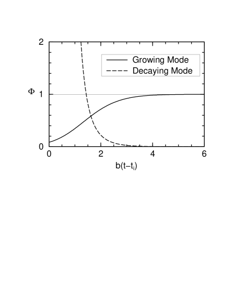
Clearly, (13) is a decaying mode, and therefore of not much importance in the evolution of fluctuations, whereas a discussion of (14) shows that $\Phi>0$ and $\dot{\Phi}>0$ for this base solution, hence it is a growing mode. Taking the two modes (13) and (14), a straightforward calculation of the conserved quantity (1) then shows $\zeta=0$ for the decaying mode, but $\zeta=1$ for the growing one.

5 Conclusions

The ‘conservation law’ (1) for cosmological perturbations indeed is a useful relation describing the growth of fluctuations of the metric in the long-wavelength limit outside the horizon, and it is derived from the correct equations of motion. It has been shown that the important growing modes always yield a non-zero value for the conserved quantity $\zeta$, both on general grounds and in an explicitly solvable toy model. The situation $\zeta=0$, when (1) can not be used to make any statement on the growth of metric perturbations in the long-wavelength limit, can occur only for decaying modes, which do not play a significant rôle in the evolution of cosmological perturbations.

After completion of this work a preprint appeared [1997] in which similar conclusions concerning the validity of Grishchuk [1996] are reached.

References

- [1965] Abramowitz M., Stegun I. A., 1965, Handbook of Mathematical Functions, Dover, New York
- [1996] Caldwell R. R., 1996, Class. Quantum Grav. 13, 2437
- [1995] Deruelle N., Mukhanov V. F., 1995, Phys. Rev. D52, 5549
- [1994] Grishchuk L. P., 1994, Phys. Rev. D50, 7154
- [1996] Grishchuk L. P., 1996, in Sánchez N., Zichichi A., eds, String Gravity and Physics at the Planck Scale. Kluwer, Dordrecht, p. 369
- [1997] Martin J., Schwarz D. J., 1997, The influence of cosmological transitions on the evolution of density perturbations, preprint gr-qc/9704049
- [1992] Mukhanov V. F., Feldman H. A., Brandenberger R. H., 1992, Physics Reports 215, 203
- [1996] Salopek D. S., 1996, in Sánchez N., Zichichi A., eds, String Gravity and Physics at the Planck Scale. Kluwer, Dordrecht, p. 409