Cumulants as non Gaussian qualifiers

Abstract

We discuss the requirements of good statistics for quantifying non-Gaussianity in the Cosmic Microwave Background. The importance of rotational invariance and statistical independence is stressed, but we show that these are sometimes incompatible. It is shown that the first of these requirements prefers a real space (or wavelet) formulation, whereas the latter favours quantities defined in Fourier space. Bearing this in mind we decide to be eclectic and define two new sets of statistics to quantify the level of non-Gaussianity. Both sets make use of the concept of cumulants of a distribution. However, one set is defined in real space, with reference to the wavelet transform, whereas the other is defined in Fourier space. We derive a series of properties concerning these statistics for a Gaussian random field and show how one can relate these quantities to the higher order moments of temperature maps. Although our frameworks lead to an infinite hierarchy of quantities we show how cosmic variance and experimental constraints give a natural truncation of this hierarchy. We then focus on the real space statistics and analyse the non-Gaussian signal generated by points sources obscured by large scale Gaussian fluctuations. We conclude by discussing the practical implementations of these techniques.

I Introduction

One of the primary goals of cosmology is a complete characterization of the seeds that led to the formation of structure. From an accurate understanding of the statistics of fluctuations we may be able to glean information about the physical origin of these seeds, their evolution and even find a precise measure of the parameters that characterize the space-time on which they live. A laboratory from which we can obtain detailed estimates is supplied by the cosmic microwave background (CMB). Much effort has focused on optimal estimates of the fluctuations’ power spectrum given the harsh realities of experimental data; one is faced with foreground contamination, incomplete sky coverage, and instrumental noise, which have to be incorporated into data analysis. A simplifying assumption has been that fluctuations in the CMB are Gaussian, allowing the development of sophisticated techniques for estimating cosmological parameters.

With current developments in experimental CMB physics, we will now be in a position to analyse very large data sets, with information about large patches of the sky measured with very high resolution and sensitivity. This means that we are in a position to seriously test some of the assumptions that have gone into the techniques that have been developed, in particular, whether the sky is really Gaussian. If the sky is Gaussian indeed, then current techniques for estimating the power spectrum will become watertight methods. Should deviations from non-Gaussianity be detected, clearly one should start again. Furthermore the power spectrum would then not be the end of the story in the quest for a statistical characterization of the fluctuations.

In the past this task has been tackled in a variety of ways subject to very different philosophies. One approach has been to choose a statistic which is easy to describe for a Gaussian random field and then try to quantify, by means of this statistic, what are the chances that a given data set comes from an underlying Gaussian ensemble. The well known examples are peaks’ statistics [1, 2], topological tests [3, 4], the 3-point correlation function [5] and skewness and kurtosis [6]. Another approach has been to devise statistics which are good discriminators between Gaussian skies and specific non-Gaussian rivals. Such is the case in much of the techniques involved in looking for topological defects [7], such as strings and textures or even foregrounds, such as point sources.

These approaches have their merits. Non-Gaussian tests are very easy to implement even in the context of very large data sets. Also reducing the whole issue to a single statistic allows one to concentrate on devising the statistic ideally suited for detecting a given, pre-known, type of non-Gaussianity. This is somewhat reminiscent of pattern recognition: if we already know what we are looking for, we may improve our chance of detecting an existing predefined pattern inside a noisy data-set.

One can, however, take a more humble approach, which is to admit that we have little idea of what the underlying probability distribution function of the CMB is. It then becomes necessary to devise as complete a framework as possible, without prejudices with regards to testing rival models, or ease of computation with regards to testing non-Gaussianity. This is an alternative approach, which supports as its underlying philosophy the quest for ruling out or detecting ${\it generic}$ non-Gaussianity.

The most well established formalism following this alternative philosophy is the n-point formalism. We briefly describe this formalism. Consider the CMB anisotropies, $\frac{\Delta T}{T}({\bf x})$ to be statistically isotropic random field, defined on the sky. We consider CMB data in the small angle limit, when projecting onto a planar patch is suitable. Since data may come in either real or Fourier space we want to address the problem of non-Gaussianity in terms of both representations. We shall use the convention:

$$\frac{\Delta T({\bf x})}{T}={\int{d{\bf k}\over 2\pi}a({\bf k})e^{i{\bf k}\cdot{\bf x}}}$$ (1)

The $n$-point correlation function is defined as the expectation value of the product of any $n$ temperatures. Translational and rotational invariance make redundant the position of one of the points and the direction of another. Hence the $n$-point function may be written as a function of $(x_{2},{\bf x}_{3},\cdots,{\bf x}_{n})$ in the form

$$C^{n}(x_{2},{\bf x}_{3},\cdots,{\bf x}_{n})={\langle\frac{\Delta T({\bf x}_{1})}{T}...\frac{\Delta T({\bf x}_{n})}{T}\rangle}$$ (2)

The 2-point correlation function and its Fourier transform, the angular power spectrum $C(k)$, are well-known. The angular power spectrum may be generalized for $n>2$ by Fourier analysing the $n$-point function

$$C^{n} (x_{2},{\bf x}_{3},\cdots,{\bf x}_{n})=$$ (4)

$$\int\frac{dk_{2}}{(2\pi)^{1/2}}\cdots\frac{d{\bf k}_{n}}{2\pi}C^{n}(k_{2},\cdots,{\bf k}_{n}){e^{ik_{2}x_{2}}\cdots e^{i{\bf k}_{n}\cdot{\bf x}_{n}}}$$

In spite of all its success it is argued in [8] that this framework is not systematic and is plagued by redundancy. In principle, one can calculate an infinite number of n-point functions, and there is no criteria where to truncate such an evaluation. If one has a finite data set, then many of these quantities will be algebraically dependent on each other. There is a practical additional problem: to estimate the m-point correlation function, one needs ${\cal O}(N_{pix}^{m})$ operations, clearly a large number for the expected large data-sets.

A possible remedy to these problems was outlined in [8]. Here we follow up on this work, but along a rather different angle. We wish to set up a practical non-redundant formalism for encoding generic non-Gaussianity, but to start with all we define are the requirements an ideal such formalism would satisfy. We then look at the formats in which data comes, and within the available descriptions we try to accommodate our requirements the best we can. The outcome is necessarily an eclectic mixture of techniques. These, we hope, will be practical devices subject to as little prejudice as possible.

II Requirements for the ideal statistics

Five major requirements will ensure that the chosen quantities afford a sensible statistical description of the random field. Depending on the particular data set available, and on the particular theory one beloves, one may give more or less emphasis to each of these requirements.

A Invariance

An essential requirement is that any statistic one defines is rotationally and translationally invariant. If we define our data set to be a set of pixels $\{\Delta T({\bf x})\}$ and the statistic $\cal G$ to be a functional then

$${\cal G}[\Delta T(R{\bf x}+{\bf a})]={\cal G}[\Delta T({\bf x})]$$ (5)

The reason underlying this criterion is the assumption that the CMB can be described as a statistically isotropic random field. The ensemble of all data sets $\{\Delta T({\bf x})\}$ remains the same under rotations and translations. Therefore it is convenient to define statistics which, when applied on a given realization, do not change if rotations and translations are performed upon this realization. By doing so we are probing more realizations in the ensemble, since the ensemble, being isotropic, replicates each realization into all the realizations related by the symmetry transformation. A good example of this requirement being enforced is the angular power spectrum $C_{\ell}$ which is independent of the way in which the axes are defined.

This requirement is essential in the standard Big Bang cosmology and within all-sky experiments, but there may be grounds for dropping it otherwise. If we look at small patches of the sky, then the existence of an observation window is already breaking the translational and rotational invariance. Also a few examples of fundamentally anisotropic fluctuations have been discussed in the past [10, 11, 9].

In the light of this argument we shall enforce this requirement in the construction in Section IV but not in the construction in Section V.

B Statistical independence for a Gaussian process

Another requirement is that any set of statistics that one defines is made up of quantities which, for a Gaussian theory, are statistically independent, and that one of these quantities be the power spectrum (which completely describes a Gaussian theory). In fact if some of the quantities we define are dependent then we are over counting degrees of freedom along which the theory is allowed to be non-Gaussian.

Such a framework was proposed in [8], where one provides a transformation from the Fourier space values of the temperature anisotropies into a complete set of independent quantities. This has the advantage of identifying the correct amount of information that one can correctly assess from a finite data set.

This requirement may however be satisfied in practice, for large data sets, even if not in theory by the formalism. A large data set will be an assumption we shall make in this paper in order to satisfy this criterion.

C Scale dependence

It has become clear that different physical processes are important on different physical scales. These different processes may have very different statistical properties. For example, the distribution of point sources will be a Poisson process, while for high wavenumbers the surface of last scattering will have an exponentially suppressed power spectrum. If one were to look at the sky at sub arc minute scales, any given pixel would be the sum of these two Gaussian and non-Gaussian distributions. It is often the case that the Gaussian component dominates the non-Gaussian one on some scales but not on others. It is therefore desirable to define statistics which are scale dependent. In the application given in the Section VI we show how this feature may be decisive in the ability of any statistic to pick subtle non-Gaussian features.

D Additivity

It may be useful if the statistics we define are additive, in the sense that if $\Delta T_{1}({\bf x})$ and $\Delta T_{2}({\bf x})$ are maps coming from two independent random processes then the statistic $\cal G$ will satisfy

$${\cal G}[\Delta T_{1}({\bf x})+\Delta T_{2}({\bf x})]={\cal G}[\Delta T_{1}({\bf x})]+{\cal G}[\Delta T_{2}({\bf x})]$$ (6)

Lack of additivity is one of the shortcomings of the formalism in [8].

Additivity may be useful firstly because one may sometimes want to combine information on different scales. For instance a given effect may be present in a band of scales, within which the power spectrum may vary, rather than in just a single scale. For instance in [8] one finds a set of transverse spectra which in the language of $a^{\ell}_{m}$ complement the power spectrum $C_{\ell}$ (which tells us how much power there is on the scale $\ell$) with a transverse spectrum $B^{\ell}_{m}$, which tells us how the power on the scale $\ell$ is distributed in angle $m$. Such an approach has the problem that few modes may then contribute to the $B^{\ell}_{m}$. Better still would be to find a truly transverse spectrum $B_{m}$ which would average over a certain range of scales $\ell$ for a fixed direction $m$. Such a $B_{m}$ spectrum would be truly orthogonal to the power spectrum $C_{\ell}$ description. Such construction cannot be provided by [8] because the quantities defined there are not additive. For additive statistics, however, extending non-Gaussian spectra over scales to non-Gaussian spectra over bands of scales is a trivial operation. Such a construction is described in Section V.

Another motivation for additivity comes from networks of non-Gaussian structures which are a Poisson process of individual non-Gaussian structures. Such networks are often globally complicated but their individual components are simple. For instance a cosmic string network is a bit of a mess globally, but is made up of essentially simple elements, say segments of Brownian strings. It is for this reason that the formalism in [8] is really better suited for small fields, where the number of non-Gaussian objects is never larger than one. For a large field [8] provides a rather complicated description. Again an additive statistic would not encounter this problem. If the individual object has a simple description within the formalism, then the same would be true for a network of such objects. Another way to phrase this concern is to say that it is useful to define statistics sensitive to local rather than global features.

We will show in Section VI this criterion at work in the context of point source subtraction. Point sources in large fields are globally complicated but locally extremely simple. We shall enforce this criterion in this context by combining two tools. Firstly we shall make use of additive cumulants. Secondly we shall introduce the concept of scale by means of the local wavelet transform.

E Computational efficiency

There are practical considerations. As mentioned above, estimating higher order statistics within the n-point formalism is very demanding on computation capabilities. One needs efficient methods which will be manageable with future million pixel data sets and available computer resources.

Related to this issue is the quest for comprehensive but non-redundant statistics. This is sometimes a problem. One can show that a distribution may be Gaussian up to a very large moment and then be non-Gaussian (although the opposite is not possible, see [12]). An infinite and largely repetitive series of moments is therefore required for completeness. We will see however how cosmic variance provides a natural cut-off for what in principle is a infinite series of statistics. The idea is that if cosmic variance goes above a given level there is no practical way in which we could detect non-Gaussianity, given the fact that we only have one sky.

F Overall picture

As one would expect, it is difficult to reconcile all these requirements. Some of them are even incompatible. For example, statistical independence leads one to work in Fourier space, where statistical isotropy and homogeneity enforce statistical independence of the different modes. On the other hand, Fourier space is a very non-local transformation, and so any statistic defined in Fourier space will be sensitive to the global properties of the sample. As stated before this may entail the awkward recognition of globally complicated networks of essentially simple components. Enforcing translational invariance, while keeping additivity, is also impossible to do in Fourier space.

We will start from a simple idea: to refine the notion of one point distribution function of $\frac{\Delta T}{T}({\bf x})$ in such a way as to incorporate as many of these requirements as possible. The fundamental idea is to calculate cumulants, or combinations of cumulants defined on various transforms on the data sets. Depending on the priorities, these transforms will be in real space or Fourier space. There are different ways in which this simple idea may be implemented. Different alternative will lead to favouring some of the above properties over others. It will be instructive to consider a few alternatives.

III Histograms and Cumulants

We will take as our starting point the one-point distribution function of $\frac{\Delta T}{T}({\bf x})$. If we were to consider an ensemble of realizations, we would be able to characterize this distribution completely. By inspecting the $\frac{\Delta T}{T}({\bf x})$ histogram of realizations one can then see if the distribution function is Gaussian or not. However, the histogram is but a graphical device. The algebraic statement corresponding to this non-Gaussianity test consists of studying the cumulants.

The cumulants of a sample (or of a distribution) are first introduced in an attempt to achieve additivity. We can define the $r^{th}$ moment of the $\frac{\Delta T}{T}({\bf x})$ distribution to be

$$\mu_{r}(\frac{\Delta T}{T})=\langle(\frac{\Delta T}{T})^{r}\rangle$$ (7)

and from Eq. (2) we see that $\mu_{r}=C^{r}(0,\cdots,0)$. The moments, if they exist, fully quantify the distribution as they appear as coefficients in the Taylor expansion of the characteristic function $\phi(t)$ (the characteristic is essentially the Fourier transform of the distribution function). The characteristic satisfies $\phi_{A+B}=\phi_{A}\phi_{B}$ and so the $\mu_{r}$ cannot be generally additive. The idea behind the definition of cumulants consists of writing down polynomials in the $\mu_{r}$ which are additive, $\chi_{r}(A+B)=\chi_{r}(A)+\chi_{r}(B)$. The prescription is defined in [12] and consists simply of taking the logarithm of the characteristic $\psi=\log\phi$. Then $\psi_{A+B}=\psi_{A}+\psi_{B}$. If $\psi$ is expanded in power series one obtains, as coefficients, a series of additive moments or cumulants $\chi_{r}$. Moments and cumulants may be related by comparing the expansions of $\psi$ and $\log\phi$. In general cumulants may be obtained from the moments using

$$\chi_{r}=r!\sum_{k=1}^{r}(-1)^{k+1}{{1}\over k}\sum_{\nu_{1}=1}^{r-k+1}\cdots\sum_{\nu_{k}=1}^{r-k+1}{\mu_{\nu_{1}}\over\nu_{1}!}\cdots{\mu_{\nu_{k}}\over\nu_{k}!}$$ (8)

where the indices $\nu_{i}$ must satisfy $\nu_{1}+\cdots+\nu_{k}=r$. At this point one notices that we get more than what we bargained for. For a Gaussian $\psi(t)=-\sigma^{2}t^{2}$ and so the cumulants of a Gaussian must be zero for $r>2$. This is an added benefit over the moments, which are not zero for a Gaussian for even orders, but instead have the relatively complicated spectrum of values:

$$\mu_{2r}={(2r)!\mu_{2}^{r}\over 2^{r}r!}=(2r-1)!!\mu_{2}^{r}=(2r-1)(2r-3)...5\times 3\mu_{2}^{r}$$ (9)

Formula (8) is not the best way to compute cumulants from the moments. An efficient algorithm is given in [12], where it is shown that

$$\chi_{r}=(-1)^{r-1}\left|\begin{array}[]{cccccc}\mu_{1}&1&0&0&\cdots&0\\ \mu_{2}&\left(\begin{array}[]{c}1\\ 0\end{array}\right)\mu_{1}&1&0&\cdots&0\\ \mu_{3}&\left(\begin{array}[]{c}2\\ 0\end{array}\right)\mu_{2}&\left(\begin{array}[]{c}2\\ 1\end{array}\right)\mu_{1}&1&\cdots&0\\ \cdots&\cdots&\cdots&\cdots&\cdots&1\\ \mu_{r}&\left(\begin{array}[]{c}r-1\\ 0\end{array}\right)\mu_{r-1}&\left(\begin{array}[]{c}r-1\\ 1\end{array}\right)\mu_{r-2}&\cdots&\cdots&\left(\begin{array}[]{c}r-1\\ r-2\end{array}\right)\mu_{1}\end{array}\right|$$ (27)

Dimensionless quantities may be constructed out of the cumulants

$${\bar{\chi}}_{r}={\chi_{r}\over\mu_{2}^{r/2}}$$ (28)

of which the familiar ${\bar{\chi}}_{3}$ and ${\bar{\chi}}_{4}$ are known as the skewness and kurtosis.

The quantities $\chi_{r}$ and $\bar{\chi}_{r}$ have two useful properties, regardless of the sample on which they are defined. Firstly they are zero for a Gaussian probability distribution function. If one considers the $\bar{\chi}_{r}$s then one can quantify this in a way which is independent of the power spectrum. Secondly the $\chi_{r}$s are are additive. This means that if $\frac{\Delta T}{T}$ is the sum of many different processes, its cumulants will be the sum of the cumulants of each process. One can’t have both of these properties, and depending on the situation we will opt to work with $\chi_{r}$ or $\bar{\chi}_{r}$.

There are a few subtleties which should be considered when working with these statistics and we will bear them in mind throughout the paper. Firstly, care must be taken when estimating these quantities from a limited sample. The simplest procedure is to define first estimators for the moments

$${\hat{\mu}}_{r}=\frac{1}{N}\sum_{i}\left(\frac{\Delta T}{T}\right)^{r}_{i}$$ (29)

where hat denotes an estimator and $N$ is the number of pixels used in the estimation. We can then use Eq. (8) or (27) to define estimators for the cumulants ${\hat{\chi}}_{r}$. It turns out that these estimators aren’t centered, i.e. $\langle{\hat{\chi}}_{r}\rangle\neq 0$ for a Gaussian distribution. The value of the bias is a function of $N$ and in the case where one has large $N$ this is not a problem. On the other hand, for small samples, one can construct unbiased centered estimators of the cumulants using what are known as $\kappa$-statistics. The idea is to bypass estimating the moments and define polynomials in the $\frac{\Delta T}{T}$ which do average to the cumulants. For the purpose of this paper we will always consider the large N limit. In the discussion we will consider the limitations of such an assumption.

There is an interesting, well known connection that can be made between cumulants and the connected Greens functions of statistical physics. In the latter case one is interested in quantifying the corrections that will be introduced if one modifies a Gaussian theory (a theory where the action can be written as a Gaussian functional on the fundamental fields) by introducing modifications. This can be done by looking at the connected Greens functions of the theory, which are simply the difference between each Green’s function of the non-Gaussian theory and the Green’s function of that order if one assumes the theory is Gaussian (using Wick’s theorem). The cumulants will be the zero lag values of these connected Green’s functions.

Finally, there is one important point that must be addressed which may be a shortcoming of any technique which uses cumulants as the basis of non-Gaussianity. If we work out the covariance matrix for cumulants we find that it is not strictly diagonal. However we find that

$$\langle{\hat{\chi}}_{r}{\hat{\chi}}_{r^{\prime}}\rangle=\frac{r!}{N}\sigma^{2r}\delta_{rr^{\prime}}+{\cal O}(\frac{1}{N^{2}})$$ (30)

The structure of the off-diagonal terms is simple to understand, in light of Wick’s theorem: if $r+r^{\prime}$ is odd, covariance is strictly zero while if $r+r^{\prime}$ is even, it is proportional to $1/N^{2}$. This means that in the limit of large $N$ (the realm of large data sets we are considering in this paper) the set of cumulants are a set of independent quantifiers of non-Gaussianity. The structure of the covariance matrix also gives us a prescription at which we can truncate, in $r$ the set of cumulants we should calculate for a given data set. By defining a maximum variance allowed we constrain $r!/N$ to be less than some value, thereby truncating the cumulants series at some value $r$.

IV Real Space Statistics

Having defined cumulants we now address the issue of the sample on which they should be computed. This depends largely on the type of data one starts from and even so there are several avenues that could be pursued. In this Section we will work towards a framework within which to work with cumulants whenever the data is provided in real space.

We are interested in probing the statistical properties of the data set at different scales, in such a way that the statistics at different scales are independent of each other as well as attempting to make them sensitive to local properties of the map.

As a first attempt at quantifying the properties of the one point distribution function one can estimate the cumulants of the pixels of one data set. Defining the estimators for the moments as above, one finds that statistical dependence of the data points increases the variance of each estimator. It can be shown that the largest term in $1/N$ in the variance of these estimators is modified by a factor. I.e. we have

$$\langle|{\hat{\chi}}_{r}|^{2}\rangle\simeq\frac{r!}{N_{eff}}\sigma^{2r}$$ (31)

where

$$\sigma^{2}=C(0)$$ (32)

$N_{eff}$ is defined to be

$$\frac{\sigma^{4}}{N_{eff}}=\frac{1}{N^{2}}\sum_{i,j}\langle T_{i}T_{j}\rangle^{2}=\frac{1}{V^{2}}\int d^{2}x\int d^{2}x^{\prime}W({\bf x})W({\bf x^{\prime}})C({\bf x},{\bf x^{\prime}})$$ (33)

where V is the sample area and $W$ is the correspnding window function. This is clearly a problem: the pixels are correlated and therefore the effective number of independent pixels is smaller than the actual number of pixels.

As discussed in the introduction, statistical isotropy, homogeneity and Gaussianity lead to the statistical independence of $\frac{\Delta T}{T}$ for different wavenumbers. It is also natural to expect that different physical processes will predominate at different scales. So ultimately one would like to define a statistics out of the cumulants which are scale dependent. In the following we present three alternatives and argue that the last one has the most advantages

A Filtered cumulants

We would like to define a linear transformation that will take the data and filter out everything but the scales of interest. We shall consider the simplest case for the moment: a real space filter which filters everything but a band of width $\sigma_{q}$ around a wave-mode $q$. In Fourier space this corresponds to a top-hat function

$${\tilde{W}}_{q}(k)=\left\{\begin{array}[]{ll}\frac{1}{\pi q\sigma}&\mbox{if $|q-k|<\frac{\sigma}{2}$}\\ 0&\mbox{otherwise}\end{array}\right.$$ (36)

The corresponding transformation in real space is given by

$$T({\bf x}) = \int dy^{2}W_{q}(|{\bf x}-{\bf y}|)T({\bf y})$$ (37)

$$W(r) = \frac{1}{4\pi\sigma q}\{q[J_{1}(q_{+}r)+J_{1}(q_{-}r)]+\frac{\sigma}{2}[J_{1}(q_{+}r)-J_{1}(q_{-}r)]\}$$ (38)

with $q_{\pm}=q\pm\frac{\sigma}{2}$ If we want to keep the number of modes constant per ring, we have $\sigma\propto q^{-1}$, i.e. $N$ constant.

The procedure can then be the folowing: given a dataset with a certain number of pixels and geometry, we can identify the number of independent scales to be probed. For simple geometries this is straightforward (the size and Nyquist frequency give us the range of modes allowed). For each wavenumber we perform this transformation using window function eq. 38 to obtain a new set of values withthe same size as the original. We then define estimators of the moments using Eq. 29 and find the cumulants using eq. 27. This quantites have some of the desired properties. Firstly they are stratifying the information in terms of scales and quantifying the non-Gaussianity in these bands in wavenumber. Secondly, both the convolution and the estimators are rotationally invariant so the final results are independent of the axis of orientation on which you are working. Thirdly, the window functions are chosen to be orthogonal, so one can decouple the information between rings. So for a given two rings with different wavenumbers, $k$ and $k^{\prime}$, the cumulants of one ring, ${\hat{\chi}}_{r}(k)$, will be independent of the cumulants of the other, ${\hat{\chi}}_{r^{\prime}}(k^{\prime})$.

There are strong shortcomings with this approach however. Firstly it is a highly non-local operation on the data set. The Fourier transform will is very sensitive to the global properties and geometry of the data and it is difficult to separate out what is truly non-Gaussian and what is due to large scale sampling effects. Of course this just means that one has to be careful when analysing the cumulants of the large wavelength modes but any form of anisotropy in the sky coverage may corrupt this analysis down to very small scales. Secondly it is a very inefficient transformation. For each wavenumber we produce a set of N points on which we define the estimators. The fact that the statistics is defined on these N points is misleading: for a filter with a wavenumber $k$ one should have approximately $N_{k}=f_{sky}(2k+1)$ independent points, much less than N. This will manifest itself if we introduce the correction into eq. 31 with $C(r)$ replaced by

$$C_{k}(r)=W^{2}_{k}\star C(r)$$ (39)

where $\star$ indicates convolution.

B Cumulants of continuous wavelet transforms

We are interested in defining a set of linear transformations that filter information in fourier space but at the same time keep information about localization. We can see the Fourier representation as one extreme, where we operate on the whole data-set, so that each Fourier value is very non-local. The other extreme is configuration space representation, where the basis vectors are $\delta$-functions on the pixels.

There is a framework within which one can have basis functions which are both localized in Fourier space and in real space. These are called wavelets [13]. In brief the idea is the following. One can expand a function $f$ in terms of a set of basis functions:

$$f({\bf x})=\sum_{l,j}{\tilde{f}}({\bf x}_{l},k_{j})\varphi_{l,j}({\bf x})$$ (40)

where the index $j$ labels the frequency band one is exploring, and the label $l$ labels the position band one is probing. These functions are compactly or almost compactly supported in real space, so they evaluate local features. One can construct these functions from a basic building block, the parent function, $\varphi({\bf x})$ through a set of translations and dilations. This parent function must satisfy an admissibility condition

$$\int\varphi(x)dx=0$$ (41)

A good example, for our purpose is that of the Maar wavelet in two dimensions:

$$\varphi({\bf x})=(2-x^{2})e^{-\frac{x^{2}}{2}}$$ (42)

To generate a family of functions with the same features we define

$$\varphi_{l,j}({\bf x})=\varphi(\frac{{\bf x}-{\bf x}_{i}}{k_{l}})$$ (43)

A transform of the data is then

$$\frac{\Delta\tilde{T}}{T}({\bf x}_{l},k_{j})=\int d^{2}x\frac{\Delta T}{T}({\bf x})\varphi_{l,j}({\bf x})$$ (44)

The transform is isotropic and one can estimate, given a mode $k$ that the numebr of points ${\bf x}_{i}$ one should obtain is ${\tilde{N}}\simeq\frac{V}{k^{2}}$, much less than in the previous section. It is also true that the quasicompact support of these functions avoid problems with the irregular geometries that one faces with just a straight Fourier transform. For a given wavenumber one simply packs the transformed regions in such a way as to avoid the boundaries.

Although this is a considerable improvement in many respects to a full Fourier transform there is one problem. As yet there is no systematic way of defining an orthonormal set of functions. The prescription described above will generate a very large number of basis functions which are all interdependent. This means that, if we define the cumulants for each band in wavenumber and use eq. 29 where we replace the sum over pixels by the sum over the spatial coefficients of the transform (the ${\bf x}_{l}$’ in eq. 44) then not only will cumulants within one ring be correlated, but cumulants within adjacent rings will be correlated.

C Cumulants of discrete wavelet transform

It turns out that there is framework within which one construct an orthonormal set of functions. One can define a set of functions in one dimension:

$$\varphi_{j,i}=2^{\frac{j}{2}}\varphi(2^{j}-i)$$ (45)

where $\varphi(x)$ satisfies the admissability condition in one dimension. These functions are orthonormal. To complete the basis one needs an additional function which satisfies $\int dx\phi(x)=1$ to contain information about the low frequency modes. Then any function can be expanded in terms of $\varphi_{i,j}$ and $\phi_{i}(x)=\phi(x-i)$. There is a certain freedom in constructing such a set of functions but Daubechies has proposed an efficient algorithm for such a purpose, which we shall outline. To define $\varphi(x)$ and $\phi(x)$ one can solve a set of equations:

$$\phi(x) = \sum_{i}c_{i}\phi(2x-i)$$ (46)

$$\varphi(x) = \sum_{i}(-1)^{1-i}c_{1-i}\phi(2x-i)$$ (47)

$$|c_{i}|^{2} = 2-\frac{(2D-1)!}{(D-1)!2^{2-2D}}\int_{0}^{i}\sin^{2D-1}xdx$$ (48)

The integer D dictates the size of the compact support of the wavelet and also indicates the regularity of the wavelet (i.e. the number of coefficinets which are zero in the Taylor expansion of each wavelet).

These functions have the properties that we have been looking for. They are local (they have compact support in real space) so one becomes insensitive to global features of the sample. They are orthonormal so one is separating information between different modes. This transform is efficient and will not give us redundant information; from $N$ pixels we will obtain $N$ coefficients. As yet, no higher dimensional analogue of this transfrom has been developed with the same useful properties. We can, however, construct 2-dimensional wavelets using the tensor products of one dimensional wavelets i.e.

$$\phi_{i_{1},i_{2}}(x_{1},x_{2}) = \phi_{i_{1}}(x_{1})\phi_{i_{2}}(x_{2})$$ (49)

$$\varphi_{i_{1},i_{2};j_{1},j_{2}}(x_{1},x_{2}) = \varphi_{i_{1};j_{1}}(x_{1})\varphi_{i_{2};j_{2}}(x_{2})$$ (50)

$$\xi^{1}_{i_{1},i_{2};j_{1}}(x_{1},x_{2}) = \varphi_{i_{1};j_{1}}(x_{1})\phi_{i_{2}}(x_{2})$$ (51)

$$\xi^{2}_{i_{1},i_{2};j_{2}}(x_{1},x_{2}) = \phi_{i_{1}}(x_{1})\varphi_{i_{2};j_{2}}(x_{2})$$ (52)

In using this approach we can now define rotationally and translationally invariant estimators for the moments. We define

$${\hat{\mu}}^{r}(k)=\sum_{i_{1},i_{2}}\sum_{j_{1},j_{2}}\left(\frac{\Delta T}{T}\right)^{r}_{i_{1},i_{2};j_{1},j_{2}}\ \ \ \mbox{where $2^{-j_{1}}+2^{-j_{2}}=k$}$$ (53)

and then use eq. 27 to define the cumulants.

V Fourier Space Statistics

For the sake of completeness we shall now discuss a possible application of cumulants to interferometric measurements, i.e. data in Fourier space [14]. Fourier mode cumulants allow an alternative formulation of the ring spectra as defined in [8]. The construction in [8] is based on dividing Fourier space into rings (scales) with $\Delta k=1$. In each ring live a total number $N(k)=2kf_{\rm sky}$ of modes $\{a({\bf k})\}$ (counting the real and imaginary parts separately) which are all independent for any Gaussian theory. In this formula $f_{\rm sky}$ is the fraction of sky covered by the experiment. The statistical independence of these modes is a mere implication of the orthogonality of the Fourier functions, and is in contrast with a real space formulation, where pixels are generally correlated. Statistical independence facilitates computing the effective number of independent modes, avoiding the trouble described in Section IV. In the same spirit, and following [15] one can define an uncorrelated mesh of independent Fourier modes. The effective number of independent modes within a mesh cell centred on $\bf{k}_{i}$ is given by

$\displaystyle\widetilde{N}_{\rm cell}(\bf{k}_{i})=1/\int_{\rm cell}{d^{2}\bf{k}\over A_{\rm cell}}\{{\rm cor}[a_{s}(\bf{k}_{i}),a_{s}^{*}(\bf{k})]\}^{2},$where $A_{\rm cell}$ is the area of the mesh cell. Clearly, $\widetilde{N}_{\rm cell}(\bf{k})$ is always greater than unity. One can therefore, on average, avoid the loss of non-redundant information by computing the average density of independent modes around a given mode at $\bf{k}=\bf{k}_{i}$

$\displaystyle\rho(\bf{k}_{i})=1/\int d^{2}\bf{k}\{{\rm cor}[a_{s}(\bf{k}_{i}),a_{s}^{*}(\bf{k})]\}^{2},$and defining the mesh size as $k_{0}=1/{\sqrt{\rho}}$. In this way estimators of statistics derived from large regions of the $\bf{k}$-plane have the same variance whether one uses the mesh or the continuum of modes in its calculation. The size of the mesh cell is $k_{0}\approx 2\pi/L$ for a square patch with size $L$, whereas for the Gaussian window of an interferometer it is $k_{0}={\sqrt{2\pi}}/\sigma_{w}$ where $\sigma_{w}$ is the variance of the Gaussian (so that its FWHM is $\theta_{w}\approx 2.3\sigma_{w}$).

Let us now look at the real and imaginary parts of the mesh modes living in each ring with $\Delta k=1$. We may then compute the cumulants of this sample $\chi_{r}(k)=\chi\{\Re a({\bf k}),\Im a({\bf k})\}$. thereby producing a two index spectrum $\chi_{r}(k)$. This spectrum includes the power spectrum ($r=2$) but also complements it with information on how the power is distributed in each ring, encoded in the $r>2$ components. In the language of [8] they complement a $C_{\ell}$ spectrum with a set of $B^{\ell}_{m}$ telling us how the power is distributed between all the modes in the ring (in direction and phase). Hence the $r$ dimension of the $\chi_{r}(k)$ spectrum may be seen as a ring spectrum, as the one proposed in [8].

The cumulants $\chi_{r}(k)$ share some of the properties given before for real fields. They can be estimated from ${\hat{\chi}}_{r}(k)$ as before. Their covariance matrix of the estimators for a Gaussian process takes the form:

$$\langle{\hat{\chi}}_{r}(k){\hat{\chi}}_{r^{\prime}}(k^{\prime})\rangle=\delta_{kk^{\prime}}{\left(\frac{r!}{N(k)}\mu_{2}^{r}\delta_{rr^{\prime}}+{\cal O}(\frac{1}{N^{2}})\right)}$$ (54)

The result for the power spectrum ($r=2$) is well known

$$\langle{\hat{\chi}}_{2}(k){\chi}_{2}(k^{\prime})\rangle=\delta_{kk^{\prime}}\frac{2}{N(k)}$$ (55)

Up to $1/N^{2}$ all that changes is the coefficient $2$ in this formula, as we go to higher order cumulants. The new coefficient is $r!$ so the variance of higher order cumulants increases very quickly. By requiring that this variance be smaller than a given value we impose a data-reduction criterion, which ensures that we will end up with a number of $\chi_{r}(k)$ smaller than $N(k)$ for each $k$.

Cumulants have advantages over the variables $\theta$ defined in [8]. To begin with they are additive. This enables computing angular spectra in bands, rather than rings, thus profiting from an enlarged number of modes. This technique leads to what is essentially direct filtering in Fourier space. It also allows the definition of something like a $B_{m}$ rather than a $B^{\ell}_{m}$, which is in a way a more orthogonal description to the power spectrum $C_{\ell}$. On the other hand cumulants have a disadvantage over the variables $\theta$ defined in [8]: their distribution for a Gaussian is not simple. All we have computed for them is a covariance matrix, which is clearly not the end of the story, because their distribution is not Gaussian. The variables $\theta$ on the other hand are simply uniformly distributed. Also the variables $\theta$ can never exceed in number the initial number of modes, whereas a cosmic variance criterion must be introduced for cumulants in order to introduce a truncation.

Unfortunately the ring cumulants $\chi_{r}(k)$, although invariant under rotations, are not invariant under translations. What is even worse, their average square variation under translations is always comparable to their variance for a Gaussian process, even for large $N(k)$. For simplicity we shall illustrate this with the moments ${\hat{\mu}}_{r}(k)$. Their variance can be easily shown to be of order:

$$\sigma^{2}({\hat{\mu}}_{r}(k))=\frac{\mu_{2r}-\mu_{r}^{2}}{N(k)}$$ (56)

Under translations the real and imaginary parts of each mode get rotated by and angle equal to $\delta\phi={\bf k}\cdot{\bf t}$ mod $2\pi$. For a uniformly distributed translation this induces an average change in ${\hat{\mu}}_{r}(k)$ of the order of $\delta{\hat{\mu}}_{r}(k)/\delta\phi$. This is of course zero. However the mean square of the change in ${\hat{\mu}}_{r}(k)$ is

$${\langle{\left({\delta{\hat{\mu}}_{r}(k)\over\delta\phi}\right)}^{2}\rangle}=\frac{2r^{2}(\mu_{2r-2}\mu_{2}-\mu_{r}^{2})}{N(k)}$$ (57)

comparable to (56). We may regard this as a problem, or not. Measurements in Fourier space usually use small fields. Small fields break translational invariance by the mere existence of a window.

A Fourier space filtering

One can take advantage of the fact that measurements are in Fourier space to perform direct filtering in Fourier space. As we have emphazised there are situations where the non-Gaussian signal is contaminated by a Gaussian signal. It may further happen that the signal non-Gaussianity is better isolated in Fourier space, that is, non-Gaussianity dominates in some scales and is dominated in others, with a clear separation of these two regimes. If data is in Fourier space in the first space then all we should do is find a window $W(k)$ defining the band where non-Gaussianity is the purest.

Again the cumulants additivity will help to quantify the effect this has on the cumulants. Let us compute cumulants of a sample made up of the real and imaginary parts of all the modes inside a given band, weighed by a window $W(k)$. Such a quantity could be related to the ring estimators ${\hat{\chi}}_{r}(k)$ by

$${\hat{\chi}}_{r}(W)=\int dk\,{N(k)W(k)\over N(W)}{\hat{\chi}}_{r}(k)$$ (58)

where $N(W)$ is the total number of modes in the band. It would therefore average to

$$\chi_{r}(W)=\int dk\,{N(k)W(k)\over N(W)}{\chi}_{r}(k)$$ (59)

If the signal is purely non-Gaussian and it involves a non-zero average cumulant which does not change sign over the band, then extending the sample over the whole band simply accumulates non-Gaussian signal in the cumulant. One is simply integrating a function which does not change sign over a domain thereby making the result more different than zero.

Furthermore the confusion with a Gaussian process also decreases because the error bars around zero for a Gaussian process also get smaller if one uses the whole band as a sample. It is easy to see that for a Gaussian random field

$$\sigma^{2}({\hat{\chi}}_{r}(W))={r!\mu_{2}^{r}\over N(W)}$$ (60)

For the very simple reason that we have more modes inside the band than inside each ring the error bar around zero for a Gaussian is much smaller for a band than for any ring.

For these two reason it makes sense computing band cumulants rather than ring cumulants. In work in progress we make use of this technique in the search of cosmic strings by interferometers [16].

B Connection with real space statistics

Finally we should add that the ring moments $\mu_{r}(k)$ and cumulants $\chi_{r}(k)$ allow a quick connection to some simple real space statistics based on histograms of temperature derivatives. If the non-additive moments are used these can be related to the Fourier transform of the $n$-point correlation function using (1):

$$\mu_{r}(\partial_{i}\cdots\partial_{j}\frac{\Delta T}{T})=\int\frac{dk_{2}}{(2\pi)^{1/2}}\cdots\frac{d{\bf k}_{n}}{2\pi}i^{r}k_{i}\cdots k_{j}C^{r}(k_{2},\cdots,{\bf k}_{r})$$ (61)

The $\mu_{r}$ of temperature derivatives can therefore be connected with the the $n$-point correlation function $C^{n}(k_{2},\cdots,{\bf k}_{n})$ but not with the ring moments $\mu_{r}(k)$. These $\mu_{r}$ are promising as they integrate over the redundant degrees of freedom in the $n$-point function $C^{n}(k_{2},\cdots,{\bf k}_{n})$.

Using the cumulants on the other hand one has

$$\chi_{r}(\frac{\Delta T}{T})=\int dk\,2\pi k\chi_{r}(k)$$ (62)

or for the temperature derivatives

$$\chi_{r}(\partial_{i}\cdots\partial_{j}\frac{\Delta T}{T})=\int dk\,i^{n}k_{i}\cdots k_{j}2\pi k\chi_{r}(k)$$ (63)

We see that the $\chi_{r}$ of the temperature derivatives consist of integrals of ring histograms $\chi_{r}(k)$ subject to different weighting powers of $k$. These powers of $k$ can be seen as a Fourier space filter. In fact, what the Fourier space filtering for cumulants, which advocated above, is doing is generalizing these statistics to filters other than power laws in $k$.

This immediately suggests a way to convert Fourier space filters into real space statistics. For filters other than power laws one obtains linear operations on the temperature maps other than the derivatives, but the practical procedure is essentially the same. Let $W(k)$ define the ring where non-Gaussianity is the purest. We may then define the optimized statistic

$$\chi^{opt}_{r}=\int dk\,2\pi kW(k)\chi_{r}(k)$$ (64)

This filter may then be inverted into a real space statistic by means of

$$\chi^{opt}_{r}=\chi_{r}(\frac{\Delta T}{T}\star W(x))$$ (65)

where $W(x)$ is the Fourier transform of the window $W(k)$.

VI An Application

To illustrate the use of the method in real space we shall construct a simple example: a Gaussian CMB signal superposed onto a Poisson distribution of point sources. As mentioned above, for certain frequencies, and for high resolution, the power spectrum of the Gaussian signal is exponentially damped due to the finite thickness of the surface of last scatter. The point source distribution, however will be white noise and so may dominate on small scales. We then have a signal dominated on large scales by the Gaussian source which may obscure the small scale non-Gaussianity. This is an ideal scenario in which to apply our technique.

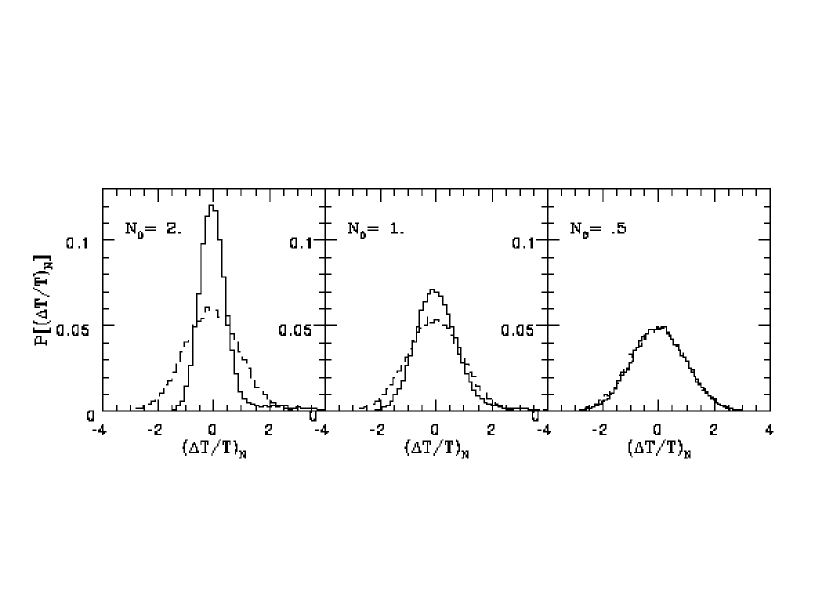
FIG. 1.: Histograms of pixels for three relative amplitudes ($N_{0}$). In each case the temperature distributions are normalized to unit variance.

FIG. 2.: The power spectra of both the Gaussian (solid line) and non-Gaussian (dashed line) signal.

,

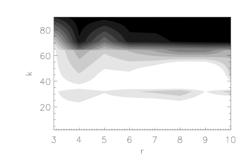
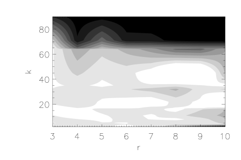
FIG. 3.: The excess variance of $\chi_{r}(k)$, $E_{r}(k)$ (left panel) and ${\bar{\chi}}_{r}(k)$, $E_{r}^{N}(k)$ (right panel). The contour lines are at .1, .2 $\cdots$ 1. , from black to white.

Considerable work has been done in finding the statistical properties of a field generated by a set of point sources [17, 18] which has led to the widely used “$P(D)$” approach. We shall use the basic ingredients described in this work to construct the non-Gaussian source. We shall generate a Poisson distribution of sources in the sky, in which the number of sources with intensity $S$ per steradian is given by a simple fit

$$N(S)=\left\{\begin{array}[]{ll}0&\mbox{$S<S_{0}$}\\ \kappa S^{-\beta}&\mbox{otherwise}\end{array}\right.$$ (68)

For purpose of illustration we shall use $\beta=1.5$. (for our purposes $k$ and $S_{0}$ will mostly affect the overall normalization). In [17, 18] an expression for the probability distribution function of the fluctuations was derived as a function of these parameters. However we are interested in the additional complication of superposing a Gaussian signal. The signal we shall use has a power spectrum

$$C_{G}(k)=A\exp(-(k/k_{d})^{2})$$ (69)

Therefore the full signal is given by

$$\frac{\Delta T}{T}=\frac{\Delta T}{T}_{ps}+\frac{\Delta T}{T}_{G}$$ (70)

where $ps$ ($G$) label the point source (Gaussian) components. We choose to fix $A$ and $k_{d}$ from

$$N^{2}_{0} = \frac{<\left(\frac{\Delta T}{T}\right)_{ps}^{2}>}{<\left(\frac{\Delta T}{T}\right)_{G}^{2}>}$$ (71)

$$N^{2}_{\infty} = \lim_{k\rightarrow 0}{{C_{ps}(k)}\over{C_{G}(k)}}$$ (72)

By varying $N_{0}$ and $N_{\infty}$ we can enhance or supress the non-Gaussian signal. In Fig. 1 we can see how the shape of the pixel distribution changes as we change $N_{0}$ ($N_{\infty}=.2$ is kept fixed). The solid line (a histogram of pixels generated as in Eq. 70) gradually merges with the dashed line (a histogram of pixels of a Gaussian realization with the same power spectrum). As argued above, the large scale Gaussian fluctuations are dominating the small scale behaviour of the non-Gaussian signal, and it is necessary to find the region where this is possible. We choose to explore with the configuration of maximum confusion, (illustrated in the right hand panel). The parameters are then $N_{0}=0.5$ and $N_{\infty}=0.2$ and we show a comparison of the power spectra in Fig. 2. Given the way we normalize the signal we have found that the statistics we are analysing in this section are essentially insensitive to different values of $\beta$.

,

FIG. 4.: One $\sigma$ regions for $V_{r}$ (left panel) and $V^{N}_{r}$ (right panel). The solid band corresponds to the Gaussian maps and the hatched band to the non-Gaussian maps.

FIG. 5.: One $\sigma$ regions for $V_{4}^{N}$ the kurtosis (suitably normalized). The horizontal, hatched region corresponds to the Gaussian.

To get a detailed understanding of the statistics we generate an ensemble of 10000 maps (of $128^{2}$ pixels) using Eq. 70 and the same number of Gaussian realizations with the same power spectrum. A natural thing to look at is the variance of both $\chi_{r}(k)$ and ${\bar{\chi}}_{r}(k)$; in fact it is instructive to plot the excess variance of the non-Gaussian distribution with regards to the Gaussian. One can define

$$E_{r}(k) = \frac{\sigma_{G}[\chi_{r}(k)]}{\sigma_{NG}[\chi_{r}(k)]}$$ (73)

$$E^{N}_{r}(k) = \frac{\sigma_{G}[{\bar{\chi}}_{r}(k)]}{\sigma_{NG}[{\bar{\chi}}_{r}(k)]}$$ (74)

and in Fig 3 we present a contour plot for both these quantities. Clearly for large wavenumbers, (for $k>65$), the non-Gaussian distribution has a large excess variance as compared to the Gaussian one ($E_{r}$ becomes less than $0.2$ very rapidly). For small wavenumbers there is confusion. The fact that we can pick up such a large difference is due to the fact that we are looking at the scales where the non-Gaussian signal dominates and we are using a set of statistics which preserves local information.

If we now focus on a band at high wavenumbers we can see the difference between the two distributions in more detail. It is useful to define

$$V_{r} = \chi_{r}(k)\times\sqrt{\frac{N_{eff}}{\sigma^{2r}r!}}$$ (75)

$$V^{N}_{r} = {\bar{\chi}}_{r}(k)\times\sqrt{\frac{N_{eff}}{r!}}$$ (76)

Note that, for a Gaussian distribution, the variance of $V_{r}$ should be proportional to $\sigma^{r}$ while the variance of $V^{N}_{r}$ is one. In Fig. 4 we plot the $68\%$ confidence regions for these two quantities for $k=70$. The excess variance, again is manifest and there is a strong signal of non-Gaussianity.

From Fig. 4 we can see that there is a value of $r$ for which the two bands do not overlap. It corresponds to the (appropriately normalized) kurtosis of the distribution. If we concentrate on $V_{4}^{N}$ as a function of scale we see that, as we expect, for low wavenumbers the two distributions are indistinguishable while for wavenumbers larger than $k=65$ there is a large discrepancy (see Fig.5). The same cannot be said about $V_{3}^{N}$, the skewness.

One may learn important lessons from this example. Introducing a scale into our statistics was clearly a good idea. Making a pure histogram of pixels was found hopeless, but filtering the data into a hierarchy of scales allowed the recognition of the point sources, by inspecting the appropriate band of scales. In that band two types of fingerprints were found for point sources. For the kurtosis there is clearly a positive average, with no overlapping cosmic variance error bars with a Gaussian process. For higer order cumulants the signal is more subtle. Although these cumulants still average to zero they show an abnormally large spread. Therefore in most realizations one would find a value for the cumulant well outside the Gaussian cosmic variance error bar, even though averaging over realization still leaves a zero cumulant. This is an example of a situation where the variance errorbar is more important than the average quantity. These two signatures are clear and strong indications of the point source non-Gaussianity.

Another important lesson is the advantage of recognizing local rather than global features. The signatures found above do not get complicated by adding more and more point sources. They are essentially dependent only on the non-Gaussian features of the individual structures. This is an advantage over the treatment of point sources given in [8], which was really only simply when there was a single point source inside the field (a situation common in the very small field context analyzed in that paper). The non-Gaussian spectra defined in [8] recognize global rather than local shapes. Hence if there were many point sources in the field they would recognize the angles between the lines connecting the various point sources, and the lenghts of all the segments, rather than the point sources themselves. For instance if there were three point sources in the field the formalism would react to the shape and size of the triangle depicted. This is naturally a complete mess for a Poisson process, even though the individual objects are very simple. The formalism used in this section, on the other hand, always recognizes individual structures. This is achieved both by the use of the wavelet transform, and the use of additive cumulants, and is a desirable feature whenever the trees are simple but the forest is complex.

VII Discussion

In this paper we have developed a new technique for quantifying non-Gaussianity using cumulants. Although in Section V we have discussed the possibility of using these quantities on interferometric data, we have focused on applying it to real space data. In this setting we have defined a set of statistics which are scale dependent, rotationally invariant and which are computationally easy to evaluate. In the limit of large data sets they are statistically independent for a Gaussian random field. One has the option of working with power spectrum independent quantities or additive quantities depending on preferences. This work is the first step in defining a useful set of statistics for analysing the future large data sets from ground and space based CMB experiments. The next steps are obvious and we shall discuss the prospects of each.

We have taken the large$-N$ limit of our data sets and this has allowed us to define simple estimators and find the simple structure of the covariance matrix in Eq. 30. Although this is the case of satellite experiments, ground based experiments in the near future may not satisfy this condition. It becomes necessary then to analyse the case of moderate $N$ and a number of problems arise. To begin with the estimators defined in Eq. 29 are biased and not centred. This means that the ${\hat{\chi}}_{r}$s won’t have zero expectation values for a Gaussian process. However, as mentioned above there is a standard procedure for dealing with this using $k-$statistics, i.e. defining statistics which have the correct expectation value. The problem then arises that the covariance matrix loses its simple form. In particular the off-diagonal terms become non-negligible. In the same way that the dependence in $r$ and $N$ gave us a criteria for truncating the number of moments to calculate, one can now impose the condition of effective diagonalization. I.e by defining a how large the off-diagonal terms are allowed to be relative to the diagonal one again obtains a constraint on $r$ given $N$. An alternative, slightly more convoluted approach is to construct linear combinations of the ${\hat{\chi}}_{r}$ so that the covariance matrix becomes diagonal. The interpretation of these new quantities is less clear.

The formalism we have developed is applicable in the small angle limit, when the sky can be approximated by a plane. Given the existence of an all sky data set (from the COBE satellite) and the expected results from the planned satellite missions, it is necessary to extend this construction to the spherical spaces. Although there has been some progress in developing wavelet techniques on arbitrary surfaces, work on fast discrete wavelet transforms in such setting is still in its infancy. There have been some proposals [20] and the current rate of progress is such that efficient algorithms will be available in the near future.

We have considered a simple example with which to illustrate our technique. In considering a non-Gaussian signal from a distribution of point sources we have made contact with the $P(D)$ approach of [17, 18]. Indeed, as mentioned in Section III cumulants are the algebraic way of characterizing a distribution. By looking at the $P(D)$ one is essentially looking at a histogram of temperature fluctuations and as we have argued, calculating the cumulants is the natural next step.

We have restricted ourselves to the two dimensional fields of temperature anisotropies. However the estimators we have defined here can be defined in any dimensions. Such situations have been explored in [19] where the statistical properties of Ly$\alpha$ clouds (one dimensional data sets) were studied in some detail. One could also envisage performing the same sort of analysis on three dimensional fields, such as the distribution of matter in the universe [21]. Indeed with the planned large scale surveys of galaxies it should be possible to characterize the distribution of density perturbation with unprecedented precision.

REFERENCES

- [1] J. R. Bond and G. Efstathiou MNRAS 226 655-687 (1987)
- [2] N. Vittorio and R. Juskiewicz Astrophys. J. 314 L29-L32 (1987)
- [3] P. Coles MNRAS 234 509-531 (1988)
- [4] J. R. Gott et al Astrophys. J. 352 1-14 (1990)
- [5] Kogut et al, Astrophys. J. 464 L29-L33 (1996)
- [6] R. Scaramella and N. Vittorio, Astrophys. J. 375 439-442 (1991)
- [7] A. Vilenkin and P. Shellard, Cosmic Strings and other Topological Defects. Cambridge University Press, Cambridge (1994);T.W.B. Kibble, J. Phys., A9 1387-1398 (1976).
- [8] P.G.Ferreira and J.Magueijo Phys. Rev. D55, 3358 (1997)
- [9] P.G.Ferreira and J.Magueijo, The closet non-Gaussianity of anisotropic Gaussian fluctuations, astro-ph/9704052.
- [10] J.Barrow, R.Juszkiewicz, Sonoda, MNRAS 213 917-943 (1985).
- [11] E.Bunn, P.G.Ferreira, J.Silk, Phys. Rev. Lett. 77 2283-2286 (1996).
- [12] M.G.Kendall and A.Stuart The Advanced Theory of Statistics, edition, Charles Griffin (1977)
- [13] I.Daubechies Wavelets, Philadelphia: S.I.A.M., (1992);M.Farge, Annu. Rev. Fluid Mech, 24, 395-457 (1992)
- [14] M.Hobson, Proceedings of the Moriond conference on CMB, (1996).
- [15] M.P.Hobson and J.Magueijo M.N.R.A.S 283, 283 (1996)
- [16] A.Albrecht, P.Ferreira, S.Hanany, A.Lewin, J.Magueijo, in preparation.
- [17] P.A.G.Scheuer, M.N.R.A.S,166, 329-337 (1974)
- [18] A.Franceschini, L.Toffolatti, L. Danese and G. De Zotti, Astrophys. J. 344 35 (1989)
- [19] L.Z. Fang and J. Pando, Proceedings of the 5th Current Topics of Astrofundamental Physics, Erice, Sicily (1996)
- [20] P.Schroder and W. Sweldens, Computer Graphics Proceedings, ACM Siggraph, 161-172 (1995)
- [21] S. Landy et al, Astrophys.J 456 L1-L4 (1996).