QSO-galaxy correlations due to weak lensing in arbitrary Friedmann-Lemaître cosmologies

Abstract

We calculate the angular cross-correlation function between background QSOs and foreground galaxies induced by the weak lensing effect of large-scale structures. Results are given for arbitrary Friedmann-Lemaître cosmologies. The non-linear growth of density perturbations is included. Compared to the linear growth, the non-linear growth increases the correlation amplitude by about an order of magnitude in an Einstein-de Sitter universe, and by even more for lower $\Omega_{0}$. The dependence of the correlation amplitude on the cosmological parameters strongly depends on the normalization of the power spectrum. The QSO-galaxy cross-correlation function is most sensitive to density structures on scales in the range $(1-10)\,h^{-1}\,$Mpc, where the normalization of the power spectrum to the observed cluster abundance appears most appropriate. In that case, the correlation strength changes by less than a factor of $\la 2$ when $\Omega_{0}$ varies between $0.3$ and $1$, quite independent of the value of $\Omega_{\Lambda}$. For $\Omega_{0}\la 0.3$, the correlation strength increases with decreasing $\Omega_{0}$, and it scales approximately linearly with the Hubble constant $h$.

1 Introduction

The existence of angular cross correlations between QSOs of moderate or high redshift with luminous foreground material on angular scales of $\ga 10^{\prime}$ has observationally been established in numerous studies. Fugmann (1990) correlated optically bright, radio-loud QSOs with Lick galaxies and found a significant overdensity of galaxies around the QSOs of some of his QSO subsamples. Bartelmann & Schneider (1993b) repeated Fugmann’s analysis with a well-defined sample of background QSOs, confirming the correlation at the $98\%$ confidence level for high-redshift, optically bright radio-QSOs. With a similar correlation technique, correlations between the 1-Jansky QSO sample and IRAS galaxies (Bartelmann & Schneider 1994) and diffuse X-ray emission (Bartelmann, Schneider, & Hasinger 1994) were investigated, yielding qualitatively the same results. Hutchings (1995) found evidence for an excess at the $\ga 5\,\sigma$ level of faint galaxies in fields of $\sim 1^{\prime}$ radius around seven QSOs with $z=2.3$.

Rodrigues-Williams & Hogan (1994) found a highly significant correlation between optically selected, high-redshift QSOs and Zwicky clusters. They discuss lensing as the most probable origin of the correlations, although simple mass models for the clusters yield lower magnifications than required to explain the significance of the effect. Seitz & Schneider (1995) repeated Rodrigues-Williams & Hogan’s analysis with the 1-Jansky sample of QSOs. They found agreement with the previous result for intermediate-redshift ($z\sim 1$) QSOs, but failed to detect significant correlations for higher-redshift sources. A variability-selected QSO sample was correlated with Zwicky clusters by Rodrigues-Williams & Hawkins (1995). They detected a significant correlation between distant QSOs and foreground Zwicky clusters, and interpreted it in terms of gravitational lensing. Again, the implied average QSO magnification is substantially larger than that inferred from simple lens models for clusters with typical velocity dispersions. Wu & Han (1995) searched for associations between distant 1-Jansky and 2-Jansky QSOs and foreground Abell clusters. They found no correlations with the 1-Jansky sources, and a marginally significant correlation with 2-Jansky sources. They argue that lensing by individual clusters is insufficient for typical cluster velocity dispersions, and that lensing by large-scale structures provides a viable explanation.

Benítez & Martínez-González (1995, 1997) found an excess of red galaxies from the APM catalog with moderate-redshift 1-Jansky QSOs on angular scales $<5^{\prime}$ at the $99.1\%$ significance level. Their colour selection ensures that the galaxies are most likely well in the foreground of the QSOs. Bartsch, Schneider, & Bartelmann (1997) re-analyzed the correlation between IRAS galaxies and 1-Jansky QSOs using a more advanced statistical technique which can be optimized to the correlation function expected from lensing by large-scale structures. In agreement with Bartelmann & Schneider (1994), they found significant correlations between the QSOs and the IRAS galaxies on angular scales of $\sim 5^{\prime}$, but the correlation amplitude is higher than expected from weak lensing by large-scale structures.

All these results indicate that there are correlations between background QSOs and foreground “light”, with “light” either in the optical, the infrared, or the (soft) X-ray wavebands. Since the foreground light emission is separated from the QSOs by typically a few hundred Mpc’s, physical associations are ruled out. Gravitational lensing is then the most likely interpretation. By the magnification bias, objects which are magnified by lensing are preferentially included in flux-limited samples. A higher than average fraction of these objects is therefore found in the background of matter overdensities. If light traces the overdensities, a correlation between foreground light and background QSOs can be established.

The angular scale of the correlations of a few arc minutes is compatible with that expected from lensing by large-scale structures, and the amplitude is either consistent with that explanation or somewhat larger (Bartelmann & Schneider 1993a). Wu & Fang (1996) discussed whether the autocorrelation of clusters modeled as singular isothermal spheres can produce sufficient magnification to explain this result. They found that this is not the case, and argue that large-scale structures must contribute substantially. In any case, the correlation scale is almost two orders of magnitude larger than the typical Einstein radius of individual galaxies. Hence, correlations on such scales cannot be attributed to the lensing effects of individual galaxies alone.

If lensing is indeed responsible for the correlations detected, other signatures of lensing should be found in the vicinity of such sources which are correlated with foreground light. Indeed, Fort et al. (1996) searched for the shear expected from weak lensing in the fields of five luminous QSOs and found coherent shear fields in all of them. In addition, they detected galaxy groups in three of their fields. Earlier, Bonnet et al. (1993) found evidence for coherent weak shear in the field of the potentially multiply-imaged QSO 2345$+$007, which was later identified with a distant cluster (Mellier et al. 1994; Fischer et al. 1994; Pelló et al. 1996).

Bartelmann (1995) has analytically calculated the angular cross-correlation function between QSOs and galaxies assuming that (i) lensing effects are weak and (ii) the biasing hypothesis of galaxy formation (e.g. Kaiser 1984; Dekel & Rees 1987) holds. This study was restricted to (iii) linear growth of density perturbations and (iv) Einstein-de Sitter (EdS) model universes. The goal of this paper is to keep assumptions (i) and (ii), but give up the restrictions (iii) and (iv). This will enable us to study the influence of cosmological parameters on the correlation function, and to assess the importance of non-linear growth of the density perturbations. Section 2 reviews the formalism, part of which is derived in appendix A. We present the results in Sect. 3 and discuss them in Sect. 4.

2 Formalism

As shown by Bartelmann (1995), the cross-correlation function $\xi_{\rm QG}(\phi)$ between high-redshift QSOs and low-redshift galaxies induced by weak gravitational lensing can be written

$$\xi_{\rm QG}(\phi)=(s-1)\,b\,\xi_{\mu\delta}(\phi)\;.$$ (1)

As mentioned in the introduction, the assumptions underlying eq. (1) are that (i) lensing effects are weak (more precisely, magnifications $|\mu-1|\ll 1$), and that (ii) galaxies are linearly biased relative to the dark matter by a factor $b$. $s$ is the double-logarithmic slope of the differential QSO number counts $n_{\rm Q}$ as a function of flux $S$, $n_{\rm Q}\propto S^{-s}$, and $\xi_{\mu\delta}$ is the angular cross-correlation function between magnification $\mu$ and density contrast $\delta$. The factor $(s-1)$ quantifies the magnification bias in eq. (1). In order to evaluate (1), we thus have to compute $\xi_{\mu\delta}$.

2.1 Cross-correlation of magnification and density contrast

A thin light bundle is sheared by the weak gravitational lensing effect of the cosmic matter distribution by the ($2\times 2$) tensor $\gamma_{ij}$ derived in eq. (LABEL:eq:A.10). Since lensing conserves surface brightness, the light bundle’s magnification is given by the inverse determinant $\det^{-1}(\delta_{ij}+\gamma_{ij})$. Dealing with weak lensing effects, we can assume $|\gamma_{ij}|\ll 1$. Therefore, the magnification $\mu=1+\delta\mu$ is

$$1+\delta\mu=[\det(\delta_{ij}+\gamma_{ij})]^{-1}\approx 1+{\rm tr}(\gamma_{ij})\;.$$ (2)

Via the trace of $\gamma_{ij}$, the magnification fluctuation contains the trace of the ($2\times 2$) Hessian $\Phi,_{ij}$ of the Newtonian potential fluctuations $\Phi$. This can be augmented by $\Phi,_{33}$ because the potential derivative along the light ray does not contribute to its deflection as long as the potential can be considered static while it is being passed by the light ray. Thus, $\nabla^{2}\Phi$ is introduced, which is related to the density contrast $\delta$ through Poisson’s equation. In comoving coordinates,

$$\nabla^{2}\Phi=\frac{3\Omega_{0}}{2a}\,\delta\;,$$ (3)

where lengths are measured in units of the Hubble length $H_{0}^{-1}c$, and the potential is scaled by $c^{2}$. With (LABEL:eq:A.10), the magnification fluctuation $\delta\mu$ becomes

$$\delta\mu(\vec{w})=3\Omega_{0}\,\int_{0}^{w}\,{\rm d}w^{\prime}\,\frac{f_{K}(w^{\prime})f_{K}(w-w^{\prime})}{f_{K}(w)}\,\frac{\delta(\vec{w}^{\prime})}{a}\;.$$ (4)

It depends on the (comoving) source distance $w$ and on the direction $(\theta_{1},\theta_{2})$ into which the light ray starts off at the observer. This is expressed in (4) by the vector $\vec{w}=[f_{K}(w)\theta_{1},f_{K}(w)\theta_{2},w]$, with the curvature-dependent radial distance $f_{K}(w)$ of (23).

The magnification fluctuation as a function of distance, $\delta\mu(\vec{w})$, has to be integrated along the line of sight, weighted by the normalized distance distribution of the sources. Let $W_{\rm Q}(w)$ be that distribution, then

$$\delta\bar{\mu}(\theta_{1},\theta_{2})=\int_{0}^{\infty}\,{\rm d}w^{\prime}\,W_{\rm Q}(w^{\prime})\,\delta\mu(\vec{w}^{\prime})\;.$$ (5)

The upper bound on the integral is to be interpreted as $w$ at $z=\infty$, which can be finite for some combinations of cosmological parameters. By changing the order of integrations, (5) can be written

$$\delta\bar{\mu}(\theta_{1},\theta_{2})=3\,\Omega_{0}\,\int_{0}^{\infty}\,{\rm d}w\,G_{\rm Q}(w)\,\frac{\delta(\vec{w})}{a}$$ (6)

with the modified weight function

$$G_{\rm Q}(w)=f_{K}(w)\,\int_{w}^{\infty}\,{\rm d}w^{\prime}\,\frac{f_{K}(w^{\prime}-w)}{f_{K}(w^{\prime})}\,W_{\rm Q}(w^{\prime})\;.$$ (7)

Likewise, the density contrast must be integrated along the line-of-sight, weighted by the distance distribution of the galaxies $W_{\rm G}(w)$ in order to get the projected galaxy number density on the sky, according to the biasing hypothesis. Hence,

$$\bar{\delta}(\theta_{1},\theta_{2})=\int_{0}^{\infty}\,{\rm d}w\,\delta(\vec{w})\,W_{\rm G}(w)\;.$$ (8)

For the shape of the weight functions $W_{\rm G}(w)$ and $G_{\rm Q}(w)$, see Fig. 1.

Both $\bar{\delta}$ and $\delta\bar{\mu}$ are projections of the three-dimensional density contrast. The density contrast is supposed to be a homogeneous and isotropic random field characterized by a power spectrum $P_{\delta}(k)$. Typical scales in $P_{\delta}(k)$ are on the order of several ten Mpc’s. The projections along the line-of-sight have length scales comparable to the Hubble radius. Under these circumstances, the Fourier-space analog of Limber’s equation can be applied (Kaiser 1992). It asserts that the power spectrum $P_{p}(\kappa)$ of a projection $p$ of a three-dimensional field $f$ with weight function $q$ is related to the power spectrum $P_{f}(k)$ of $f$ through

$$P_{p}(\kappa)=\int_{0}^{\infty}\,{\rm d}w\,\frac{q^{2}(w)}{f_{K}^{2}(w)}\,P_{f}\left(\frac{\kappa}{f_{K}(w)}\right)\;.$$ (9)

Note that $\vec{\kappa}$ is a two-dimensional wave vector, while $\vec{k}$ is three-dimensional. The cross power spectrum $P_{\mu\delta}(\kappa)$ of the density contrast and the magnification fluctuation is therefore given by

$$P_{\mu\delta}(\kappa)=3\,\Omega_{0}\,\int_{0}^{\infty}\,{\rm d}w\,\frac{G_{\rm Q}(w)W_{\rm G}(w)}{a(w)\,f_{K}^{2}(w)}\,P_{\delta}\left(\frac{\kappa}{f_{K}(w)}\right)\;.$$ (10)

The cross correlation function $\xi_{\mu\delta}(\phi)$ is the Fourier transform of $P_{\mu\delta}(\kappa)$,

$$\xi_{\mu\delta}(\phi)=\int_{0}^{\infty}\frac{\kappa{\rm d}\kappa}{(2\pi)^{2}}\,P_{\mu\delta}(\kappa)\,\int_{0}^{2\pi}d\vartheta\,\exp(-{\rm i}\,\kappa\phi\cos\vartheta)\;,$$ (11)

where $\vartheta$ is the angle enclosed by $\vec{\kappa}$ and $\vec{\phi}$. The $\vartheta$-integration yields a zeroth-order Bessel function ${\rm J}_{0}$, and inserting (10) leads to

$$\xi_{\mu\delta}(\phi) = 3\,\Omega_{0}\,\int_{0}^{\infty}\,{\rm d}w\,\frac{G_{\rm Q}(w)W_{\rm G}(w)}{a(w)}$$ (12)

$$\times \int_{0}^{\infty}\,\frac{k{\rm d}k}{2\pi}\,P_{\delta}(k,w)\,{\rm J}_{0}[f_{K}(w)k\phi]\;.$$

It should be noted that eq. (12) automatically accounts for two effects: First, matter inhomogeneities “behind” the QSOs do not contribute to the gravitational lensing effects. This can be seen by inserting $W_{\rm Q}=\delta(w-w_{\rm Q})$ into eq. (7), upon which $G_{\rm Q}\propto{\rm H}(w_{\rm Q}-w)$, with the Heaviside step function ${\rm H}(x)$. Inserting this together with $W_{\rm G}=\delta(w-w_{\rm G})$ with $w_{\rm G}>w_{\rm Q}$ into eq. (12) yields $\xi_{\mu\delta}=0$, as it should. Second, the autocorrelation of galaxies is included through the matter power spectrum $P_{\delta}(k)$.

The matter power spectrum $P_{\delta}(k,w)$ depends on time, which is expressed in (12) as a dependence on comoving distance $w$. Assuming linear growth of the density fluctuations, $P_{\delta}(k,w)=P_{\delta}^{0}(k)\,D(w)$, with the power spectrum $P_{\delta}^{0}(k)$ at the present epoch and a cosmology-dependent growth function $D(w)$. An accurate fit formula for $D(w)$ is given in Carroll, Press, & Turner (1992). In that case, the integrations over $w$ and $k$ can be separated. This yields the instructive equation

$$\xi_{\mu\delta}(\phi)=\int_{0}^{\infty}\,\frac{k{\rm d}k}{2\pi}\,P_{\delta}(k,w)\,F(k,\phi)\;,$$ (13)

which shows that the cross correlation function between magnification and density contrast is a convolution of the matter power spectrum with a filter function $F(k,\phi)$, weighted by the wave number $k$. For the Einstein-de Sitter case, $F(k,\phi)$ is plotted in Bartelmann (1995; Fig. 2). For small angles $\phi$, $F(k,\phi)$ filters out scales smaller than $\sim 1\,$Mpc. Here, we evaluate eq. (12) numerically, including the non-linear growth of $P_{\delta}(k,w)$.

2.2 Choice of the weight functions

We have to specify the QSO- and galaxy weight functions $G_{\rm Q}$ and $W_{\rm G}$. For the QSO weight function $W_{\rm Q}$, we choose a QSO redshift distribution of the form given by Pei (1994), with parameters adapted to observations in the same paper. With (7), this yields QSO weight functions $G_{\rm Q}(w)$ for which examples are given in the right panel of Fig. 1. $G_{\rm Q}$ depends on the lower redshift cutoff $z_{0}$ imposed on the QSO sample.

Figure 1: Examples for the galaxy weight function $W_{\rm G}(w)$ (left panel), and for the QSO weight functions $G_{\rm Q}(w)$ adopted from Pei (1994; right panel). All curves are shown for an Einstein-de Sitter model universe. $m_{0}$ is the detection threshold magnitude for the galaxies, and $z_{0}$ is the lower redshift cutoff of the QSO sample. Line types distinguish results for different $m_{0}$ or $z_{0}$, as indicated.

For the galaxy redshift distribution underlying the galaxy weight function $W_{\rm G}(w)$, we assume a constant comoving number density of galaxies. The galaxies are distributed in luminosity according to a Schechter luminosity function with parameters $\nu=-0.81$ and $L_{*}=1.1\times 10^{10}L_{\odot}h^{-2}$. We further choose a threshold apparent magnitude $m_{0}$ for the galaxies, which we calculate from $L$ and $w$ using a $K$-correction derived from an effective spectral energy distribution with index $\alpha=-1.5$. Examples for the resulting weight functions are given in the left panel of Fig. 1. Our results for the cross-correlation function $\xi_{\mu\delta}(\phi)$ show that $\xi_{\mu\delta}(\phi)$ depends only very weakly on the exact shape of the weight functions $W_{\rm G}(w)$ and $G_{\rm Q}(w)$, once $m_{0}$ and $z_{0}$ are fixed.

2.3 Matter power spectra

We use in the following three different types of matter power spectra $P_{\delta}(k)$, viz. cold dark matter (CDM), hot dark matter (HDM), and mixed dark matter (MDM). For each of these dark-matter types, several fitting formulae have been given in the literature. Comparing results for the QSO-galaxy cross-correlation function, we found that different formulae for the same dark-matter type yield only marginally different correlation functions. We can therefore restrict the study to one formula for each dark-matter type only. For definiteness, we use those given by Efstathiou, Bond, & White (1992) for CDM, Bardeen et al. (1986) for HDM, and Holtzman (1989) for MDM.

Semi-analytic prescriptions for the non-linear evolution of the power spectra have been given by Jain, Mo, & White (1996) and Peacock & Dodds (1996). Both rest on the conjecture by Hamilton et al. (1991) that the non-linear power on a given scale $k_{\rm nl}$ is identified with the linear power on a larger scale $k_{\rm l}$ which is some universal function of $k_{\rm nl}$. This universal function has to be identified through numerical simulations. The prescription by Peacock & Dodds (1996) works as long as the local double-logarithmic slope of the power spectrum at the scale of interest is not steeper than that of the CDM spectrum. This is not the case at small scales for an HDM power spectrum. For that, we rather use the evolution calculated in the framework of the Zel’dovich approximation by Schneider & Bartelmann (1995). For MDM, we use linear evolution only. To give an example, Fig. 2 shows the non-linear evolution of a CDM spectrum in an Einstein-de Sitter universe.

Figure 2: Comparison between the linear (dotted curves) and non-linear (solid curves) evolution of a CDM power spectrum, according to the prescription given by Peacock & Dodds (1996) for an Einstein-de Sitter model universe. Non-linear power builds up on small scales at the expense of power on intermediate scales. The linear spectra are normalized to $\sigma_{8}=1$.

One further point in specifying the power spectra is to normalize the shape predicted for the chosen matter model with measurements. There are three basic possibilities to do this. (i) Determine the variance of galaxy counts on a fixed scale, commonly $8\,h^{-1}\,$Mpc, and assume that light follows mass, with some linear bias factor $b$. (ii) Measure the abundance of galaxy clusters and fix the amplitude of the power spectrum such that this abundance is reproduced. (iii) Fix the amplitude of the power spectrum such that the amplitude of the cosmic microwave background anisotropies are reproduced. It is well known that these methods yield different amplitudes for the CDM power spectrum. It is possible to match (i) and (ii) by choosing the bias factor suitably. To also match (i) or (ii) with (iii), the shape of the power spectra needs to be changed on small scales. We emphasize here that the angular cross-correlation function between QSOs and galaxies provides in principle a more direct measurement of the matter power spectrum than counting galaxies or clusters, for it is based on gravitational lensing. We shall later demonstrate the huge effect which the non-linear growth of density fluctuations has on the amplitude of the cross-correlation function on small angular scales (Fig. 2).

We show results for all three normalizations of the power spectrum, not accounting for the further constraints that are derived from galaxy counts, galaxy autocorrelation functions, or the cluster abundance. In that way, our results can easily be scaled to the desired normalization.

3 Results

As shown by Bartelmann (1995) for the special case of a linearly evolving density field in an Einstein-de Sitter universe, the shape of the cross-correlation function $\xi_{\mu\delta}(\phi)$ depends sensitively on the type of the dark-matter particles. This property of $\xi_{\mu\delta}(\phi)$ continues to hold for all the generalizations we calculate here. We use the results obtained for linear density evolution in an Einstein-de Sitter universe as a reference for the influence of cosmological parameters and non-linear density evolution.

3.1 Dependence on type and evolution of the dark matter

Figure 3 demonstrates the different shapes of $\xi_{\mu\delta}(\phi)$ for different matter power spectra. In agreement with the analytic description of Bartelmann (1995), the cross-correlation function (left panel of Fig. 3) peaks for $\phi\to 0$, whereas it flattens off at small $\phi$ for HDM. Power-series expansion yields $\xi_{\mu\delta}\propto\phi+{\cal O}(\phi^{2})$ for CDM, and $\xi_{\mu\delta}\propto\phi^{2}+{\cal O}(\phi^{4})$ for HDM (Bartelmann 1995). The reason for this is the different asymptotic behavior of $P_{\delta}(k)$ for $k\to\infty$: the cut-off in the HDM power spectrum is responsible for the flattening of the HDM cross-correlation function. As expected, $\xi_{\mu\delta}$ for MDM falls between these two cases, in that it flattens at smaller $\phi$ than for HDM.

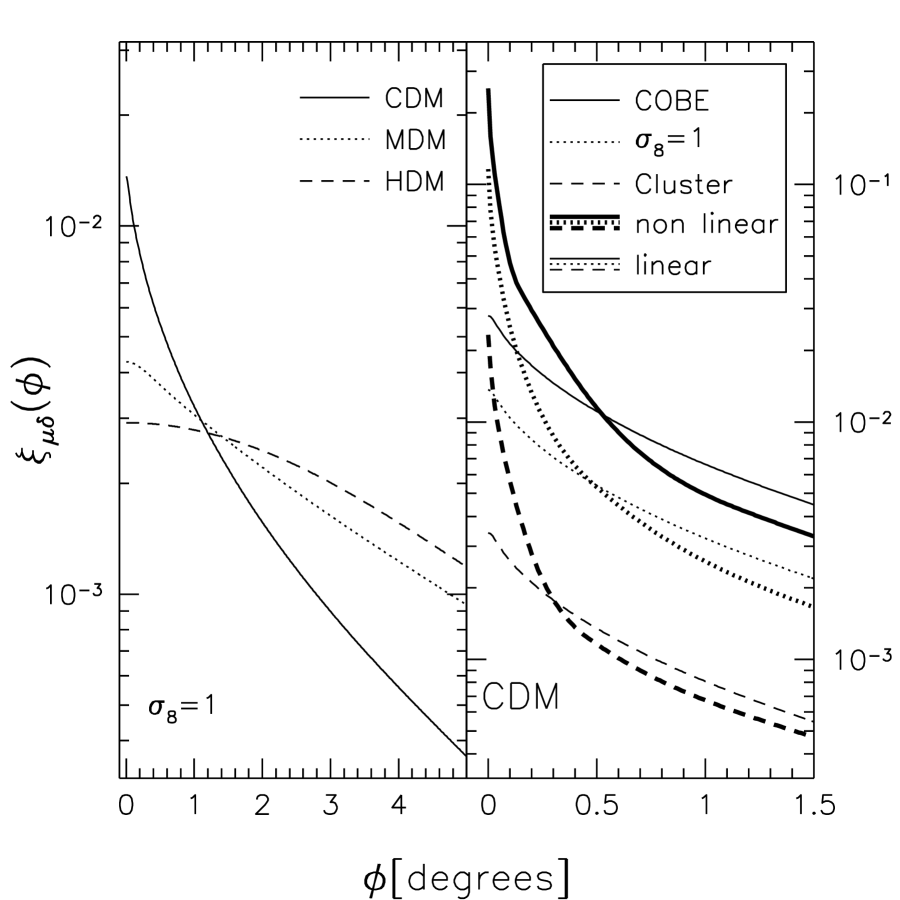
Figure 3: The cross-correlation function $\xi_{\mu\delta}(\phi)$ is shown here for an Einstein-de Sitter universe. Left panel: results for different types of linearly evolving dark-matter power spectra (CDM, solid curve; MDM, dotted curve; HDM, dashed curve). All spectra were normalized to $\sigma_{8}=1$. While the cross-correlation function peaks towards $\phi\to 0$ for CDM, it flattens for HDM and MDM due to the cut-off at large wavenumbers $k$ in those spectra. At large angles $\phi$, the HDM and MDM correlation functions lie above the CDM results. Right panel: the effect of the non-linear evolution of the CDM power spectrum on $\xi_{\mu\delta}(\phi)$, for three different normalizations, as indicated by line type. The COBE normalization yields the largest amplitude, the cluster normalization the smallest. The linear results are shown as the thin lines for comparison. For this choice of the cosmological model, non-linear evolution increases the correlation amplitude $\xi_{\mu\delta}(0)$ by about an order of magnitude, quite independent of the normalization. $m_{0}=20.5$ and $z_{0}=0.3$ were chosen.

The cross-correlation function for the different normalizations of the CDM power spectrum is shown in the right panel of Fig. 3. Clearly, the high normalization to the COBE results yields the strongest correlation, while the normalization to cluster counts yields the weakest. For small angles $\phi$, the window function $F(k,\phi)$ (see Bartelmann 1995 for details) drops to zero at the scale of galaxy clusters and smaller structures. Hence, the integral (12) yields the strongest correlation for the COBE normalization, because the COBE normalization leads to much more power on cluster scales than the cluster normalization.

The non-linear growth of the density fluctuations also most strongly affects the power on scales of clusters and smaller (see Fig. 2). Because of that, the influence of non-linear density evolution on the cross-correlation function is huge. The right panel of Fig. 3 contrasts the cross-correlation function for non-linear and linear density evolution of the power spectra. For the CDM model in an Einstein-de Sitter universe, the amplitude, $\xi_{\mu\delta}(0)$, of the cross-correlation function increases by about one order in magnitude, quite independent of the normalization. Depending on the normalization, the increase can be even larger in other model universes. Since $\xi_{\mu\delta}(\phi)$ remains unaffected on large angular scales, the peak for $\phi\to 0$ is sharpened by non-linear evolution, in tentative agreement with observations (Benítez & Martínez-González 1995; 1997). Non-linear evolution of the power spectra is, therefore, crucial to match theoretical expectations and measurements.

Non-linear evolution also increases the HDM correlation amplitude. However, the flattening of the HDM correlation function for $\phi\to 0$, and its much lower amplitude than for CDM, appears to be ruled out by observations, and we will therefore concentrate on CDM spectra in the following.

3.2 Dependence on cosmological parameters

The change of the cross-correlation function with different cosmological parameters shows a huge dependence on the normalization of the power spectrum. This is due to the fact that the three normalizations themselves depend differently on the cosmological parameters.

To understand the dependence of the correlation function on the cosmological parameters a bit better, we adapt an analytical expression by Bartelmann (1995) to our discussion. Using a CDM model spectrum, and assuming linear density evolution, Bartelmann (1995) obtains

$$\xi_{\mu\delta}(0)=\frac{3\,A_{\rm CDM}\,k_{0}^{3}}{2}\,K_{0}$$ (14)

for an Einstein-de Sitter universe. Here, $A_{\rm CDM}$ is the amplitude of the power spectrum, $k_{0}$ is the wave number of the peak in the spectrum, and $K_{0}$ is an integral over the weight functions introduced in Sect. 2.2. In non-EdS cosmologies, we get an additional factor $\Omega_{0}$ from Poisson’s equation, and $k_{0}\propto\Omega_{0}\,h$ in units of the inverse Hubble length. Using this, the dependence of the amplitude $\xi_{\mu\delta}(0)$ (for linear evolution) can be written as

$$\xi_{\mu\delta}(0)\propto\Omega_{0}^{4}\,h^{3}\times[A_{\rm CDM}]\times[K_{0}]\;,$$ (15)

where the square brackets around a symbol denote the dependence of the corresponding quantity on the cosmological parameters. Fig. 4 illustrates the dependence of $\xi_{\mu\delta}(0)$ on $h$ and $\Omega_{0}$ for various cosmological models and normalizations of the power spectrum.

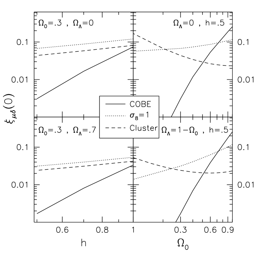
Figure 4: The dependence of the correlation amplitude $\xi_{\mu\delta}(0)$ on the Hubble constant $h$ and the matter density $\Omega_{0}$ is shown for different cosmological models and different normalizations of the CDM power spectrum. Non-linear evolution was assumed. Left panels: dependence on $h$; right panels: dependence on $\Omega_{0}$; upper panels: open models ($\Omega_{\Lambda}=0$); lower panels: spatially flat models ($\Omega_{0}+\Omega_{\Lambda}=1$). Different normalizations are distinguished by line type, as indicated. The COBE normalization yields the strongest dependence on both $h$ and $\Omega_{0}$. Generally, $\xi_{\mu\delta}(0)$ decreases with decreasing $h$ and decreasing $\Omega_{0}$, but note that the cluster normalization reverses that trend, especially for the open models (upper right panel). All curves were calculated assuming $m_{0}=20.5$ and $z_{0}=0.3$.

We looked in detail at three different cosmological models. These are: an Einstein-de Sitter universe with two different values of the Hubble constant $H_{0}$, an open low-density model with $\Omega_{0}=0.3$, and $\Omega_{\Lambda}=0$, and a spatially flat low-density model with $\Omega_{0}=0.3$ and $\Omega_{\Lambda}=0.7$. The correlation functions $\xi_{\mu\delta}(\phi)$ for these cosmologies and different normalizations are shown in Fig. 5. The left panel of Fig. 6 illustrates the dependence on $\Omega_{0}$ of the correlation amplitude $\xi_{\rm QG}(0)$ for cluster normalization. We restrict the discussion of the dependence on cosmological parameters to non-linear models only.

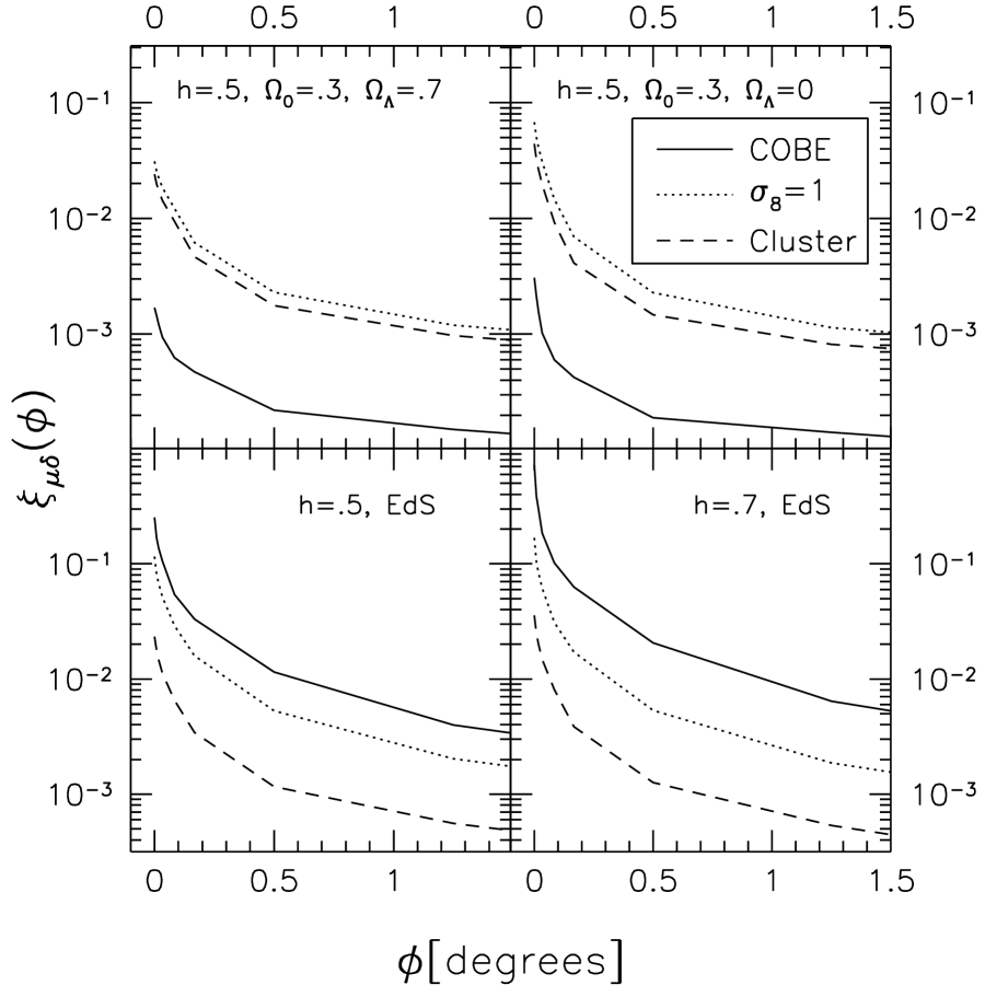
Figure 5: The angular cross-correlation function $\xi_{\mu\delta}(\phi)$ is plotted for different values of the cosmological parameters. In all panels, curves for the three normalizations are shown, distinguished by line type as indicated. Top left panel: spatially flat low-density universe with $h=0.5$, $\Omega_{0}=0.3$, and $\Omega_{\Lambda}=0.7$; top right panel: open low-density universe with $h=0.5$, $\Omega_{0}=0.3$, and $\Omega_{\Lambda}=0$; bottom panels: Einstein-de Sitter universes with $h=0.5$ (left) and $h=0.7$ (right). All curves are for CDM and for $m_{0}=20.5$ and $z_{0}=0.3$.

In an Einstein-de Sitter universe, the correlation is strongest for the COBE normalization. This changes in low-density universes, where we find a stronger correlation for the cluster- and the $\sigma_{8}=1$ normalizations. Generally, the correlation amplitude increases with $\Omega_{0}$, except for the cluster normalization. There, the correlation amplitude changes only mildly with $\Omega_{0}$ as long as $\Omega_{0}\ga 0.3$, and it increases when $\Omega_{0}$ decreases even further. Likewise, a larger Hubble constant yields a higher correlation amplitude. Both these effects are mainly due to the fact that the peak in the power spectrum shifts towards larger wave numbers with increasing $\Omega_{0}$ and $H_{0}$, and the additional factor $\Omega_{0}$ from Poisson’s equation renders a stronger dependence on $\Omega_{0}$ than on $H_{0}$. Depending itself quite strongly on $\Omega_{0}$, the cluster normalization can reverse the general trend with $\Omega_{0}$.

Approximate relations between the amplitude $\xi_{\mu\delta}(0)$ and $\Omega_{0}$ and $H_{0}$ are shown in Tab. 1. They are in good qualitative agreement with the expectations from eq. (15). Figure 4 and Tab. 1 also show that the strongest dependence on the cosmological parameters is obtained for the COBE normalization. The dependence on the cosmological constant $\Omega_{\Lambda}$ for fixed $\Omega_{0}$ is much weaker than for the other parameters, which reflects the fact that $\Omega_{\Lambda}$ affects only the space-time curvature, which enters through $K_{0}$ in eq. (15).

Table 1: This table summarizes the dependence of the correlation amplitude $\xi_{\mu\delta}(0)$ on the cosmological parameters $h$ and $\Omega_{0}$, for non-linearly evolved CDM spectra. We fitted parabolae in $\ln\xi_{\mu\delta}(0)$–$\ln Q$ space to the curves in Fig. 4, with $Q$ either $h$ or $\Omega_{0}$. Hence, we fit $\ln\xi_{\mu\delta}(0)=A\,(\ln Q)^{2}+B\,\ln Q+C$, and give the coefficients $A$, $B$ and $C$ in the table. When $h$ is varied, we take $\Omega_{0}=0.3$, $\Omega_{\Lambda}=0$ for the open models, and $\Omega_{0}=0.3$, $\Omega_{\Lambda}=0.7$ for the spatially flat models. When $\Omega_{0}$ is varied, we take $h=0.5$. The dependences differ with the normalization, hence we give results for the three normalizations we have chosen. For the cluster normalization, we also give results for the correlation amplitude $\xi_{\rm QG}(0)$, which differs from $\xi_{\mu\delta}(0)$ by the bias factor $b=\sigma_{8}^{-1}$.

		Normalization
$Q$	Coeff.	COBE	$\sigma_{8}=1$	Cluster
		$\xi_{\mu\delta}(0)$	$\xi_{\mu\delta}(0)$	$\xi_{\mu\delta}(0)$	$\xi_{\rm QG}(0)$
	$A$	$-1.2$	$0.1$	$0.1$	$0.1$
$h$	$B$	$3.7$	$0.9$	$1.0$	$1.0$
(open)	$C$	$-2.5$	$-2.1$	$-2.5$	$-1.8$
	$A$	$-1.0$	$0.1$	$0.1$	$0.1$
$h$	$B$	$3.6$	$0.9$	$0.9$	$0.9$
(flat)	$C$	$-3.5$	$-3.0$	$-3.2$	$-2.5$
	$A$	$-1.0$	$0.1$	$0.3$	$0.3$
$\Omega_{0}$	$B$	$2.5$	$0.6$	$-0.2$	$0.3$
(open)	$C$	$-1.4$	$-2.1$	$-3.7$	$-2.5$
	$A$	$-0.3$	$0.2$	$0.3$	$0.3$
$\Omega_{0}$	$B$	$3.8$	$1.3$	$0.3$	$0.8$
(flat)	$C$	$-1.4$	$-2.1$	$-3.7$	$-2.5$

3.3 Other model parameters

Quite generally, the dependence of the correlation function on all the other parameters entering our calculation is weak. As mentioned in Sect. 2.3, there is no significant change of the correlation function upon using different spectra for the same dark-matter model. Small changes in the amplitude of the angular cross-correlation function result from varying the parameters $z_{0}$ and $m_{0}$ of the weight functions introduced in Sect. 2.2. This is due to the fact that varying the mean redshift of the galaxies (through $m_{0}$), or the QSO redshift distribution (through $z_{0}$) changes the lensing efficiency. Examples are shown in the right panels of Fig. 6. The upper right panel illustrates how the correlation amplitude changes if the mean redshift of the galaxies is shifted beyond the maximum in lensing efficiency for a fixed QSO redshift distribution. The lower right panel shows how the correlation amplitude increases with increasing QSO redshift.

Figure 6: Left panel: amplitude of the angular cross-correlation function between QSOs and galaxies, $\xi_{\rm QG}(0)$, as a function of $\Omega_{0}$. The curves are for cluster-normalized, non-linearly evolving CDM in open and spatially flat model universes. Note the difference to the correlation amplitude $\xi_{\mu\delta}(0)$ between magnification and density contrast: We have assumed a bias factor of $b=\sigma_{8}^{-1}$ here. Upper right panel: dependence of $\xi_{\rm QG}(0)$ on the threshold galaxy magnitude $m_{0}$; lower right panel: dependence of $\xi_{\rm QG}(0)$ on the minimum QSO redshift $z_{0}$. While $\xi_{\rm QG}(0)$ increases monotonically with $z_{0}$, it reaches a maximum for $m_{0}\simeq 19$ and decreases for fainter galaxies. The curves in the right panels are calculated in an Einstein-de Sitter universe with cluster normalization of the power spectrum. $z_{0}=0.3$ in the upper right panel and $m_{0}=20.5$ in the lower right panel.

The fact that $\xi_{\mu\delta}(\phi)$ peaks for moderately faint galaxies rather than for the faintest can easily be understood. The galaxies are simply tracers of the density inhomogeneities that act as lenses on the QSO samples. At fixed QSO redshift, there is an intermediate redshift at which the lenses are most efficient. This redshift is somewhat reduced by the redshift dependence of structure growth. Allowing for fainter galaxies selects more distant density inhomogeneities which are less efficient lenses, making the cross-correlation function $\xi_{\mu\delta}$ drop.

4 Summary and discussion

We have extended an earlier study of the angular cross-correlation function $\xi_{\rm QG}(\phi)$ between QSOs and galaxies (Bartelmann 1995) in three respects. First, we generalize from the Einstein-de Sitter to arbitrary Friedmann-Lemaître cosmological models, second, we allow for the non-linear evolution of the density fluctuations, and third, we construct more realistic redshift distributions for galaxies and QSOs. The QSO-galaxy correlation function is expressed in terms of the correlation function between magnification and density contrast, $\xi_{\mu\delta}(\phi)$.

We confirm that the shape of the cross-correlation function is very sensitive to the type of the dark-matter power spectrum: While it peaks for $\phi\to 0$ in the case of CDM, it flattens for HDM and MDM. Measurements of $\xi_{\rm QG}(\phi)$ indicate that the correlation peaks for $\phi\to 0$, in contradiction to the flattening expected for HDM. Given further the much lower correlation amplitude for HDM compared to CDM, we focus on the CDM model.

We summarize our main results as follows:

1. Non-linear evolution of the density fluctuations leads to an increase in the correlation amplitude $\xi_{\mu\delta}(0)$ relative to the linear case by about an order of magnitude, or more.

2. $\xi_{\mu\delta}(\phi)$ depends on the cosmological parameters $\Omega_{0}$, $H_{0}$, and $\Omega_{\Lambda}$ in different ways:

   • $\Omega_{0}$ enters through Poisson’s equation, through the normalization, the shape, and the evolution of the power spectrum, and through space-time curvature. The location of the peak in the power spectrum is proportional to $\Omega_{0}\,h=\Gamma$. The larger $\Gamma$ is, the larger is the overlap between the power spectrum and the window function that filters out the scales relevant for $\xi_{\mu\delta}$. Therefore, the correlation generally becomes stronger with increasing $\Omega_{0}$, except for the cluster normalization.

   • The Hubble constant enters through the shape parameter of the power spectrum, $\Gamma=\Omega_{0}\,h$. As for $\Omega_{0}$, the correlation strengthens with increasing $H_{0}$.

   • The cosmological constant $\Omega_{\Lambda}$ enters only weakly through space-time curvature and the evolution of the power spectrum.

3. The method by which the power spectrum is normalized plays a critical role, both for the amplitude of the correlation and its dependence on cosmological parameters. When the spectrum is normalized to the COBE measurements, the dependence on cosmological parameters is strongest. For the cluster normalization, the dependence on $\Omega_{0}$ is weakest, and it can even be reversed for small $\Omega_{0}$, because the general decrease is compensated by the $\Omega_{0}$ dependence of the normalization.

4. Other parameters entering the calculation of the correlation function have a comparably modest influence. Factors of $1.5-2$ can be gained or lost by varying the galaxy detection threshold $m_{0}$ or the minimum QSO redshift $z_{0}$. The exact shape of the galaxy- and QSO redshift distributions is largely irrelevant, and different representations published in the literature for the same type of power spectrum yield the same correlation functions.

We have argued that, for small angular scales $\phi$, $\xi_{\mu\delta}(\phi)$ is most sensitive to the power on cluster scales. This is because the filter function $F(k,\phi)$ introduced in eq. (13) drops to zero on smaller scales, and the further factor $k$ in the integrand of eq. (13) suppresses the largest scales. Lacking more precise information on the true shape and normalization of the matter power spectrum on the scales relevant for the QSO-galaxy cross-correlation function, the normalization to the observed cluster abundance appears most appropriate for our purposes. The dependence of $\xi_{\mu\delta}(0)$ especially on the density parameter is then fairly weak as long as $\Omega_{0}\ga 0.3$. As Tab. 1 and Fig. 4 show, $\xi_{\mu\delta}(0)$ changes by at most a factor of $\la 2$ across that range of $\Omega_{0}$, and the dependence on $H_{0}$ is approximately linear. Figure 7 illustrates the range of QSO-galaxy cross-correlation functions $\xi_{\rm QG}(\phi)$ that can be covered by varying cosmological parameters while keeping the normalization of the power spectrum fixed to the cluster abundance. For illustration, we overplotted Fig. 7 with the observational data points by Benítez & Martínez-González (1995, 1997).

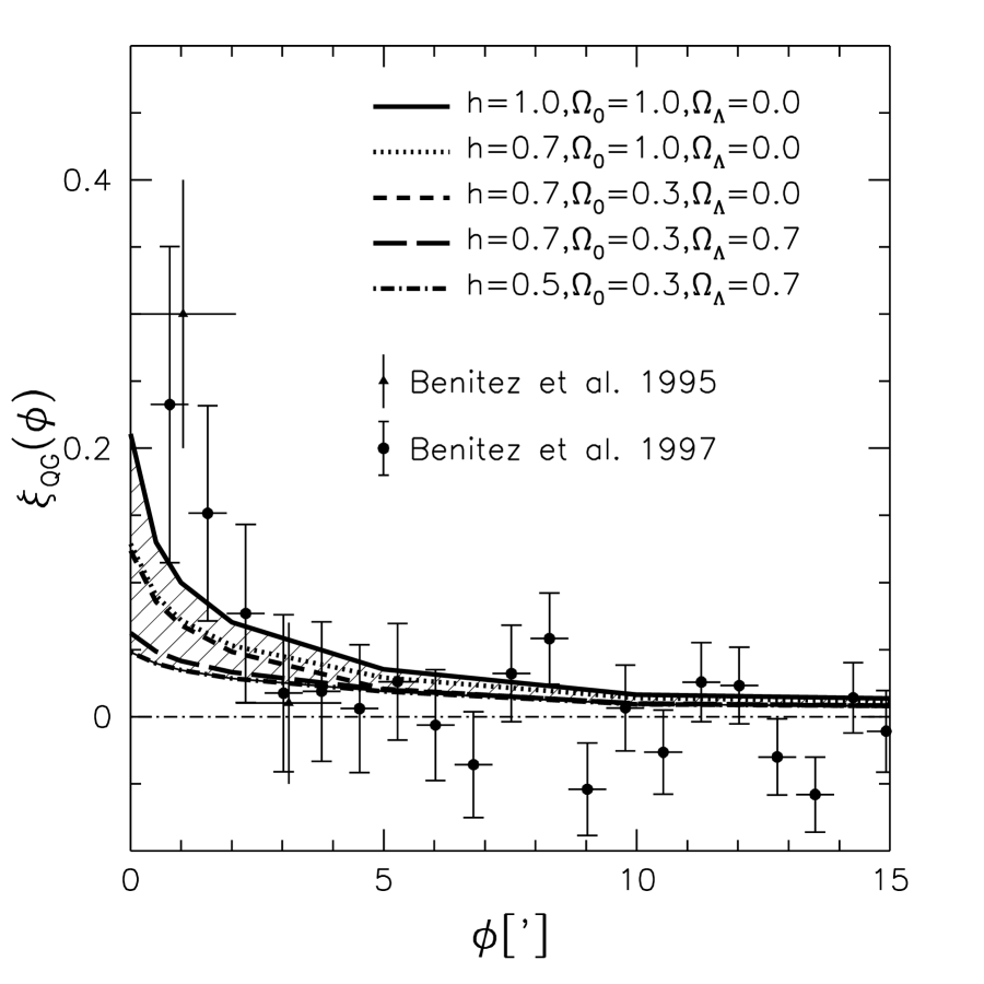
Figure 7: The range of correlation functions $\xi_{\rm QG}(\phi)$ that can be covered by varying cosmological parameters while keeping the normalization of the power spectrum fixed to the cluster abundance. As Tab. 1 and Fig. 4 show for that normalization, $\xi_{\mu\delta}(\phi)$ changes by less than a factor $\la 2$ for $\Omega_{0}\ga 0.3$, and it scales with $H_{0}$ approximately linearly. Note that we are plotting $\xi_{\rm QG}$ rather than $\xi_{\mu\delta}$ here. We have assumed $s=2.8$ (cf. Bartelmann 1995) and $b=\sigma_{8}^{-1}$ to relate the two; see eq. (1). The cluster normalization requires roughly $\sigma_{8}\approx 0.6\,\Omega_{0}^{0.6}$, hence $b\propto\Omega_{0}^{-0.6}$. See also the curves in the left panel of Fig. 6. We have further assumed $m_{0}=20.5$ and $z_{0}=0.3$, corresponding to the values chosen in Benítez & Martínez-González (1995, 1997), whose data points are added for illustration.

While non-linear structures on clusters scales are accurately represented by the non-linear power spectrum, our approach does not accurately represent the strong lensing that sets in close to cluster cores. Since we have linearized the magnification factor $\mu$ in eqs. (1) and (2), our results fail to be applicable when $\mu$ becomes noticeably larger than unity, $\mu\ga 1.5$, say. This is the case for QSOs closer than $\sim 3$ Einstein radii to a cluster core. Depending on cosmological parameters, QSO and cluster redshifts, and on the velocity dispersion of the cluster, $\sim 3$ Einstein radii correspond to $\sim 1-2^{\prime}$. That is to say that the expected QSO-galaxy correlation function calculated here should fall below the true correlation at $\phi\la 1-2^{\prime}$.

The most accurate measurement of $\xi_{\rm QG}(\phi)$ has so far been obtained by Benítez & Martínez-González (1995, 1997). They find a significant correlation at angular scales $\phi<5^{\prime}$, and a result compatible with zero at larger $\phi$. We can therefore not yet compare our results to the innermost points of the observational data. This must be postponed until $\xi_{\rm QG}(\phi)$ has significantly been detected at angles $\ga 3^{\prime}$. We note that especially the Sloan Digital Sky Survey will provide an ideal data base for this kind of analysis.

A comparable study was performed by Sanz, Martínez-Gonzalez, & Benítez (1997) while the work on this paper was completed. In a forthcoming paper, these authors will perform a detailed comparison of the data and the theoretical results.

Appendix A The cosmological shear tensor

We summarize in this appendix the derivation of the shear tensor by which the lensing effects of cosmic material deform thin light bundles. We start from the conformal Friedmann-Lemaître (FL) metric,

$${\rm d}s^{2}=a^{2}(\eta)\,\left[{\rm d}\eta^{2}-{\rm d}w^{2}-f_{K}^{2}(w)\,{\rm d}\omega^{2}\right]\,,$$ (16)

with the scale factor $a$, the conformal time $\eta$, the comoving distance $w$, and the comoving angular-diameter distance $f_{K}(w)$, which depends on the spatial curvature $K$. $\eta$ is related to the cosmic time $t$ through ${\rm d}t=a{\rm d}\eta$ with the boundary condition $\eta=0$ at $t=0$. Measuring lengths in units of the Hubble length $H_{0}^{-1}c$, and setting the scale factor at the present epoch to unity, $K$ can be written in the usual form

$$K=\Omega_{0}+\Omega_{\Lambda}-1\;,$$ (17)

where $\Omega_{0}$ is the matter-density parameter, and $\Omega_{\Lambda}$ is the density parameter attributed to the cosmological constant, both taken at the present epoch.

Consider now a fiducial light ray propagating through the space-time (16), starting off at the observer into direction $(\theta_{1},\theta_{2})$. The affine parameter $\lambda$ along the fiducial ray is chosen such that ${\rm d}\lambda=-a\,{\rm d}t$. The transverse separation vector $\vec{\xi}$ of a neighboring light ray from the fiducial ray changes with $\lambda$ according to

$$\frac{{\rm d}^{2}\vec{\xi}}{{\rm d}\lambda^{2}}=-\frac{3}{2}\,\Omega_{0}\,a^{-5}\,\vec{\xi}\;,$$ (18)

(Gunn 1967; Blandford et al. 1991; Seitz, Schneider, & Ehlers 1994). We now substitute in (18) the comoving separation vector $\vec{x}=a^{-1}\vec{\xi}$ for $\vec{\xi}$, and the comoving distance $w$ for $\lambda$. From ${\rm d}s=0$ and (16), ${\rm d}w=-{\rm d}\eta$ for radial light rays. Since ${\rm d}\lambda=-a\,{\rm d}t=-a^{2}{\rm d}\eta$, ${\rm d}w=a^{-2}{\rm d}\lambda$. After some manipulation, these substitutions yield

$$\frac{{\rm d}^{2}\vec{x}}{{\rm d}w^{2}}+K\,\vec{x}=0\;.$$ (19)

The solutions of this oscillator equation are the usual linear combinations of trigonometric (for $K>0$), hyperbolic (for $K<0$), or linear functions (for $K=0$).

Equation (19) describes the change in comoving transverse separation between two light rays on cosmic scales, $\sim H_{0}^{-1}c$. Locally, space time is perturbed by density fluctuations with Newtonian potential $\Phi$. Relative to an unperturbed light ray, such perturbations deflect light according to

$$\frac{{\rm d}^{2}\vec{x}(\vec{w})}{{\rm d}w^{2}}=-2\,\nabla_{\perp}\Phi(\vec{w})\;,$$ (20)

(e.g. Schneider, Ehlers, & Falco 1992; Narayan & Bartelmann 1997) where we have scaled $\Phi$ by $c^{2}$ and used that locally, ${\rm d}w=-c\,{\rm d}t$. $\vec{w}$ is the vector $[f_{K}(w)\theta_{1},f_{K}(w)\theta_{2},w]$. The gradient of $\Phi$ has to be taken perpendicular to the actual light ray, but for the small deflections we consider here it can be taken perpendicular to the unperturbed ray.

Equations (19) and (20) describe light deflection on completely different spatial scales. To combine the effect of the global curvature of space time with the light deflection by isolated density fluctuations, we can thus simply add the right-hand side of (20) to the right-hand side of (19). Written in components, the result is

$$\frac{{\rm d}^{2}x_{i}(\vec{w})}{{\rm d}w^{2}}+K\,x_{i}(\vec{w})=-2\,\Phi,_{i}(\vec{w})\;,$$ (21)

where the index $i$ preceded by a comma denotes the partial derivative with respect to $x_{i}$. Equation (21) is solved by

$$x_{i}(\vec{w})=f_{K}(w)\,\vec{\theta}-2\,\int_{0}^{w}\,{\rm d}w^{\prime}\,f_{K}(w-w^{\prime})\,\Phi,_{i}(\vec{w}^{\prime})\;,$$ (22)

with the boundary conditions that the unperturbed fiducial ray and the perturbed ray both start at the observer into directions separated by $\vec{\theta}$, hence $\vec{x}_{i}(0)=0$ and ${\rm d}\vec{x}_{i}/{\rm d}w=\vec{\theta}$ at $w=0$. $f_{K}(w)$ is the comoving angular-diameter distance of the metric (16),

$$f_{K}(w)=\left\{\begin{array}[]{ll}K^{-1/2}\,\sin(K^{1/2}w)&(K>0)\\ w&(K=0)\\ |K|^{-1/2}\,\sinh(|K|^{1/2}w)&(K<0)\\ \end{array}\right.$$ (23)

Recall that (22) is the comoving separation of a perturbed light ray from an unperturbed one. The net angle $\vec{\alpha}$ by which the perturbed light ray is deflected is therefore simply

$$\alpha_{i}[f_{K}(w)\theta_{1},f_{K}(w)\theta_{2},w]=\frac{x_{i}(\vec{w})-f_{K}(w)\,\vec{\theta}}{f_{K}(w)}$$ (24)

$$= -2\,\int_{0}^{w}\,{\rm d}w^{\prime}\,\frac{f_{K}(w-w^{\prime})}{f_{K}(w)}\,\Phi,_{i}(\vec{w}^{\prime})\;.$$

(Seljak 1996). Consequently, the shear exerted on a thin light bundle is

$$\gamma_{ij}(\vec{w}) = \frac{\partial\alpha_{i}[w,f_{K}(w)\theta_{1},f_{K}(w)\theta_{2}]}{\partial\theta_{j}}$$

$$= -2\,\int_{0}^{w}\,{\rm d}w^{\prime}\,\frac{f_{K}(w^{\prime})f_{K}(w-w^{\prime})}{f_{K}(w)}\,\Phi,_{ij}(\vec{w}^{\prime})\;.$$

This result agrees with that of other recent studies which focus on different lensing statistics (Seljak 1996; Jain & Seljak 1996; Bernardeau, van Waerbeke, & Mellier 1996; Kaiser 1996).

References

- [1] Bardeen, J.M., Bond, J.R., Kaiser, N., Szalay, A.S., 1986, ApJ, 304, 15
- [2] Bartelmann, M., Schneider, P., 1993a, A&A, 268, 1
- [3] Bartelmann, M., Schneider, P., 1993b, A&A, 271, 421
- [4] Bartelmann, M., Schneider, P., 1994, A&A, 284, 1
- [5] Bartelmann, M., Schneider, P., Hasinger, G. 1994, A&A, 290, 399
- [6] Bartelmann, M., 1995, A&A, 298, 661
- [7] Bartsch, A., Schneider, P., Bartelmann, M., 1997, A&A, 319, 375
- [8] Benítez, N., Martínez-González, E., 1995, ApJ, 448, L89
- [9] Benítez, N., Martínez-González, E., 1997, ApJ, 477, 27
- [10] Bernardeau, F., van Waerbeke, L., Mellier, Y., 1996, A&A, in press; preprint astro-ph/9609122
- [11] Blandford, R.D., Saust, A.B., Brainerd, T.G., Villumsen, J.V., 1991, MNRAS, 251, 600
- [12] Bonnet, H., Fort, B., Kneib, J.-P., Mellier, Y., Soucail, G., 1993, A&A, 280, L7
- [13] Carroll, S.M., Press, W.H., Turner, E.L., 1992, ARA&A, 30, 499
- [14] Dekel, A., Rees, M.J., 1987, Nat, 326, 455
- [15] Efstathiou, G., Bond, J.R., White, S.D.M., 1992, MNRAS, 258, P1
- [16] Fischer, P., Tyson, J.A., Bernstein, G.M., Guhathakurta, P., 1994, ApJ, 431, L71
- [17] Fort, B., Mellier, Y., Dantel-Fort, M., Bonnet, H., Kneib, J.-P., 1996, A&A, 310, 705
- [18] Fugmann, W., 1990, A&A, 240, 11
- [19] Gunn, J., 1967, ApJ, 150, 737
- [20] Hamilton, A.J.S., Matthews, A., Kumar, P., Lu, E., 1991, ApJ, 374, L1
- [21] Holtzman, J.A., 1989, ApJS, 71, 1
- [22] Hutchings, J.B., 1995, AJ, 109, 928
- [23] Jain, B., Seljak, U., 1996, preprint astro-ph/9611077
- [24] Jain, B., Mo, H.J., White, S.D.M., 1996, MNRAS, 276, L25
- [25] Kaiser, N., 1984, ApJ, 284, L9
- [26] Kaiser, N., 1992, ApJ, 388, 272
- [27] Kaiser, N., 1996, preprint astro-ph/9610120
- [28] Narayan, R., Bartelmann, M., 1997, in: Proc. 1995 Jerusalem Winter School, eds. A. Dekel & J.P. Ostriker. Cambridge: University Press
- [29] Mellier, Y., Dantel-Fort, M., Fort, B., Bonnet, H., 1994, A&A, 289, L15
- [30] Peacock, J.A., Dodds, S.J., 1996, MNRAS, 280, L19
- [31] Pei, Y.C., 1994, ApJ, 438, 623
- [32] Pelló, R., Miralles, J.M., Le Borgne, J.-F., Picat, J.-P., Soucail, G., Bruzual, G., 1996, A&A, 314, 73
- [33] Rodrigues-Williams, L.L., Hogan, C.J., 1994, AJ, 107, 451
- [34] Rodrigues-Williams, L.L., Hawkins, M.R.S., 1995, in: Dark Matter. AIP Conf. Proc. 336, eds. S.S. Holt & C.L. Bennett (New York: AIP)
- [35] Sanz, J.L., Martínez-Gonzalez, E., Benítez, N., 1997, preprint
- [36] Schneider, P., Bartelmann, M., 1995, MNRAS, 273, 475
- [37] Schneider, P., Ehlers, J., Falco, E.E., 1992, Gravitational Lenses. Heidelberg: Springer Verlag
- [38] Seitz, S., Schneider, P., 1995, A&A, 302, 9
- [39] Seitz, S., Schneider, P., Ehlers, J., 1994, Class. Quantum Grav., 11, 2345
- [40] Seljak, U., 1996, ApJ, 463, 1
- [41] Wu, X.-P., Fang, L.-Z., 1996, ApJ, 461, L5
- [42] Wu, X.-P., Han, J., 1995, MNRAS, 272, 705