ULTRA-HIGH ENERGY COSMIC RAY SOURCES AND LARGE SCALE MAGNETIC FIELDS

Abstract

Protons of energies up to $\sim 10^{20}\,$eV can be subject to significant deflection and energy dependent time delay in lage scale extragalactic or halo magnetic fields of strengths comparable to current upper limits. By performing 3-dimensional Monte Carlo simulations of nucleon propagation, we show how observations of arrival direction and time distributions can be used to measure the structure and strength of large-scale magnetic fields, and constrain the nature of the source of ultra-high energy cosmic rays.

astro-ph/9704203

Submitted to Astrophysical Journal Letters

1 Introduction

If extragalactic magnetic fields (EGMFs) exist, they are at a level below detectability with presently available techniques. Faraday rotation measures of distant powerful radio-sources give upper limits to extragalactic fields of $B_{\rm rms}\sqrt{l_{c}}\lesssim 10^{-9}$G Mpc^1/2, where $l_{c}$ denotes the reversal length of the field (see, e.g., Kronberg 1994). However, EGMFs below these current limits are of significant interest to cosmology, galaxy and star formation, and galactic dynamos (see, e.g., Kronberg 1994; Olinto 1997).

The propagation of UHECRs is affected by the presence of EGMFs of strength $10^{-12}\,{\rm G}\lesssim B_{\rm rms}\lesssim 10^{-9}\,{\rm G}$ and/or by Galactic halo fields $10^{-8}\,{\rm G}\lesssim B_{H}\lesssim 10^{-6}\,{\rm G}$. Protogalactic fields in the former range are actually expected if the galactic magnetic field cannot be explained by a galactic dynamo (Kulsrud & Anderson 1992). In this letter, we study how EGMFs and the halo magnetic field, which we collectively name large-scale magnetic fields (LSMFs), affect UHECRs with energies $E\gtrsim 10\,{\rm EeV}$ (EeV = $10^{18}$ eV). We simulate the propagation of ultra-high energy nucleons in the LSMF and the cosmic microwave background (CMB), and show how the resulting angle-time-energy images of these UHECRs, could be used, in turn, to probe LSMFs with strengths in the above range. Suitable UHECR statistics could be achieved with future experiments, such as the Japanese Telescope Array (Teshima et al. 1992), the High Resolution Fly’s Eye (Al-Seady et al. 1996), and the Pierre Auger Project (Cronin 1992), that have the potential to detect $\sim 10-10^{3}$ particles per source with $E\gtrsim 10^{19}$eV, over a $\sim 5\,{\rm yr}$ period. Although the origin and nature of UHECRs are not known, they are likely to be generated in extragalactic sources (e.g., Bird et al. 1995; Yoshida et al. 1995; Hayashida et al. 1996), such as powerful radio-galaxies (e.g., Rachen & Biermann 1993), cosmological $\gamma-$ray bursts (Vietri 1995; Waxman 1995; Milgrom & Usov 1996), and/or topological defects (e.g., Bhattacharjee, Hill & Schramm 1992; Sigl 1996). Our results can also be used to discriminate between models of the origin of UHECRs.

Previous studies of the effect of the LSMF on UHECRs have included a discussion of the energy dependent deflection and time delay for extragalactic UHECRs (Cronin 1992; Waxman & Miralda-Escudé 1996; Medina Tanco et al. 1997). In addition, the effect of EGMFs on secondary $\gamma$-rays produced in the interaction of ultra-high energy protons with CMB photons can also probe EGMFs below current upper limits: Plaga (1995) and Waxman & Coppi (1996) proposed to use the arrival time delay of secondary $\gamma$-rays in the TeV range to probe EGMFs of strengths $B_{\rm rms}\lesssim 10^{-15}$G, while Lee, Olinto & Sigl (1996) showed how fields of strength $B_{\rm rms}\sim 10^{-9}$G affect the $\gamma-$ray spectrum around $10\,{\rm EeV}$ due to electron synchrotron losses.

2 Angle-time-energy images

Nucleons propagating in intergalactic space with energies $\gtrsim 10\,$EeV are mainly subject to scattering on the LSMFs and pair production on the CMB (for protons), as well as photopion production on the CMB. Pair production dominates the energy loss below $\simeq 70\,$EeV which we include as a continuous loss process (Chodorowski, Zdziarski, & Sikora 1992). Above $\simeq 70\,$EeV photopion production dominates and gives rise to the Greisen-Zatsepin-Kuz’min cutoff (hereafter GZK cutoff; Greisen 1966; Zatsepin & Kuzmin 1966). We model photopion production as a stochastic process where the chance of interaction is drawn at random, as described in Lee (1996), and Sigl, Lee, & Coppi (1996). We model the EGMF as a gaussian random field, with zero mean in Fourier space, and power spectrum: $\left\langle B^{2}(k)\right\rangle\propto k^{n_{B}}$ for $k<2\pi/l_{c}$, and $\left\langle B^{2}(k)\right\rangle=0$ otherwise. Here, $l_{c}$ characterizes the cutoff scale of magnetic fluctuations; we choose $l_{c}=1\,{\rm Mpc}$ as a fiducial value for the EGMF. The power spectrum is normalized via: $B_{\rm rms}^{2}\equiv V/(2\pi)^{3}\int d^{3}{\bf k}B^{2}({\bf k})$. We leave the detail description of our Monte-Carlo code to Sigl, Lemoine, & Olinto (1997).

A simpler version of the present study was carried out by Medina Tanco et al. (1997). These authors described the field as an assembly of randomly oriented bubbles of constant field, with diameter equal to the coherence length, and neglected the stochastic nature of pion production. Finally, they considered the limit $D\theta_{E}\gg l_{c}$, where $D$ denotes the distance to the source, and $\theta_{E}$ the r.m.s. deflection angle at energy $E$; this limit is obtained only for extreme choices of the magnetic field strength and configuration for $E\gtrsim 10^{20}$eV (see below). The limit $D\theta_{E}\ll l_{c}$ is not only the most probable for $E>10^{19}$eV, it also is the most difficult to treat (see Sigl, Lemoine, & Olinto (1997). The importance of distinguishing the limits $D\theta_{E}\gg l_{c}$ and $D\theta_{E}\ll l_{c}$, was pointed out by Waxman & Miralda-Escudé (1996). In the latter limit, all nucleons emitted by the source and captured on the detector have essentially experienced the same magnetic structure along their paths, hence the scatter around the mean of the correlations between the time delay $\tau_{E}$, the deflection angle $\theta_{E}$, and the energy $E$, is of order 1%. In the opposite limit, $D\theta_{E}\gg l_{c}$, the relative widths of these correlations are of order unity.

Our simulations generate data consisting of the energy, arrival time, and angular direction for each UHECR emitted from the source. For general reference, we can estimate the average deflection angle $\theta_{E}$ and the average time delay $\tau_{E}\simeq D\theta_{E}^{2}/2c$ induced on a proton of energy $E\lesssim 50\,{\rm EeV}$ over a distance $D$ in the limit $D\theta_{E}\gg l_{c}$. Using (Waxman & Miralda-Escudé 1996):

$$\tau_{E}\,\simeq\,2.5\,\left(\frac{3+n_{B}}{2+n_{B}}\right)\left(\frac{D}{10\,{\rm Mpc}}\right)^{2}\left(\frac{E}{10\,{\rm EeV}}\right)^{-2}\left(\frac{B_{\rm rms}}{10^{-11}\,{\rm G}}\right)^{2}\left(\frac{l_{c}}{1\,{\rm Mpc}}\right)\,{\rm yr}\,,$$ (1)

and $\theta_{E}\simeq 0.014^{\circ}(D/10\,{\rm Mpc})^{-1/2}(\tau_{E}/1\,{\rm yr})^{1/2}$. The Faraday rotation bound $B_{\rm rms}\sqrt{l_{c}}<10^{-9}$G Mpc^1/2, implies $\tau_{E}\lesssim 3\times 10^{4}$ $(D/10\,{\rm Mpc})^{2}(E/10\,{\rm EeV})^{-2}\,$yr, and $\theta_{E}\lesssim 2.5^{\circ}(D/10\,{\rm Mpc})^{1/2}$ $(E/10\,{\rm EeV})^{-1}$, assuming $n_{B}\simeq 0$. In what follows, we address the possible observables for different cases. In §2.1 and §2.2, we discuss the case of an extra-galactic bursting source. In §2.3, we discuss the case of a continuously emitting source. In these sections, we consider the case in which the time delay induced by the extra-galactic magnetic field dominates over that of the halo magnetic field of our Galaxy. In §2.4, we discuss how the domination by a halo field would modify our conclusions. We use the notations $\tau_{100}\equiv\tau_{E=100EeV}$, $\theta_{100}\equiv\theta_{E=100EeV}$.

2.1 Observable time delays

The best case for probing large scale magnetic fields as well as the nature of the source is: $\tau_{50}\simeq 1\,{\rm yr}$, i.e., the time delay is comparable to the integration time of the experiment, $T_{obs}$. In this case, the limit $D\theta_{E}\ll l_{c}$ holds as the Faraday rotation bound is combined with $\tau_{50}\simeq 1\,{\rm yr}$. For a propagated differential energy spectrum ${\rm dJ}\propto E^{-\eta}{\rm d}E$, that corresponds to the injected spectrum below the GZK cutoff, Eq. (1) tells us that the arrival time distribution is given by ${\rm dJ}\propto t^{(\eta-3)/2}{\rm d}t$, for a bursting source with emission timescale $T_{S}\ll\tau_{50}$ and a $\tau_{E}-E$ correlation with negligible scatter. Note that a continuous source with $T_{S}\gg 1\,{\rm yr}$ would produce a uniform distribution of arrival times, notably independent of their energy (see §2.4).

The observation of the arrival time and energy of two events is sufficient to determine a zero-point in time (time of emission), hence the value of $\tau_{E}$, equivalently $DB_{\rm rms}\sqrt{l_{c}}$. The distance can be independently derived by fitting the energy spectrum above the GZK cutoff, provided there is enough statistics. Thus, one ends up with an estimate of the distance to the source, the nature of the source (e.g., burst vs. continuous emission), and the value of $B_{\rm rms}^{2}l_{c}$. Observations of several clusters of events would thus “map” the extra-galactic magnetic field. Finally, one can show, from $\tau_{50}\simeq D\theta_{50}^{2}/2\simeq 1\,{\rm yr}$, that the angular image would not be resolved for a typical detector with resolution $\delta\theta\gtrsim 0.5^{\circ}$. That typical time delays above tens of EeV may be of the order of a few years, is suggested by a detailed likelihood analysis (Sigl, Lemoine, & Olinto 1997) of the three pairs of events that were recently reported by the AGASA experiment (Hayashida 1996).

2.2 Large time delays

If $\tau_{E}\gg T_{obs}\sim{\rm a\,few\,yr}$, a given source will be seen only on a limited range in energy (Waxman & Miralda-Escudé 1996); indeed, protons with higher energy have already reached us in the past, while protons with lower energy have yet to reach us. These authors have derived the shape of the energy spectrum in the limit $D\theta_{E}\gg l_{c}$, for $E\lesssim 50$EeV where the signal has significant scatter $\Delta E/E\sim 30$%; in the opposite limit $D\theta_{E}\ll l_{c}$, $\Delta E/E\sim 1$%. In principle, the measure of the width would tell us which limit applies, and would give us some information about $B_{\rm rms}$ and $l_{c}$. However, this statement depends strongly on the distance, as $D\theta_{E}/l_{c}\propto D^{3/2}$. For sufficiently large time delays, the angular image of the source could be resolved for $E\lesssim 50\,{\rm EeV}$, in which case the value of $B_{\rm rms}\sqrt{Dl_{c}}$ becomes accessible. Moreover, the argument developed by Waxman & Miralda-Escudé (1996) would allow to place another constraint on these parameters, respectively $D/l_{c}\ll 1$ or $D/l_{c}\gg 1$.

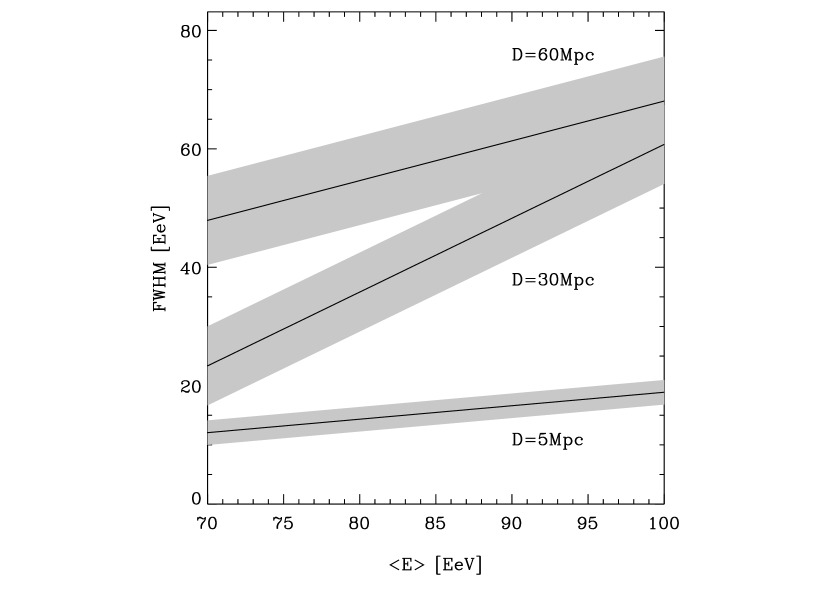
Figure 2: Full width at half maximum (FWHM) vs. the average energy, for the observed spectrum, above pion production threshold, for large time delays $\tau_{E}\gg T_{obs}$ and small deflection $D\theta_{E}\ll l_{c}$. Shown are linear fits to the correlations calculated from time slices through Figure 1 as well as the 1$\sigma$ uncertainty around these fits for different distances $D=5\,{\rm Mpc}$, $D=30\,{\rm Mpc}$, and $D=60\,{\rm Mpc}$, as indicated.

For sources that are observed above the pion production threshold, the previous statements do not apply. However, in this limit, one can use a similar reasoning to obtain an estimate of the distance. At a fixed time, only a given range of energies is observed. Intuitively, the larger the distance, the more important the pion production, hence the broader the signal. This effect is illustrated in Figures 1 and 2. Figure 1 shows the image of the source in the time-energy plane for a source lying at $D=60\,{\rm Mpc}$. The correlation $\tau_{E}\propto E^{-2}$ is shown as a dotted line. In this plane, the effect of pion production is mainly to downscatter from higher energies to lower energies, with a trend toward increasing the time delay for a given energy at emission. Figure 2 shows the correlation between the width of the signal in energy, as actually seen by the detector, vs. the mean energy of the signal. This signal is obtained as a slice in the $\tau_{E}-E$ image, integrated between $t$ and $t+T_{obs}$, where $T_{obs}=5\,{\rm yr}$ in this case and $t$ is arbitrary; this slice is indicated in Figure 1 by the dashed lines. An example of the signal in energy so obtained is shown in Figure 3 in dashed line. The correlation shown in Figure 2 was obtained by measuring the width of the signal for different mean energies, corresponding to different choices of $t$, and adjusting a straight line fit. The shaded areas denote the 1$\sigma$ range of (numerical) uncertainty. These uncertainties actually provide a hint of the actual experimental uncertainties associated with such measurements, as the number of particles used in the Monte-Carlo correspond to that expected from a typical UHECR source. As Figure 2 reveals, an estimate of the distance $5\,{\rm Mpc}\lesssim D\lesssim 100\,{\rm Mpc}$, could be achieved with reasonable accuracy. For $D\lesssim 5\,{\rm Mpc}$, the width of the signal becomes dominated by the instrumental resolution, whereas for $D\gtrsim 100\,{\rm Mpc}$, statistics should insufficient.

2.3 Continously emitting sources

The case of a continous source, emitting on a timescale $T_{S}$, is obtained by folding, on the time axis, the angle-time-energy image of a corresponding bursting source, with a top-hat of width $T_{S}$. In principle, for a given magnetic field configuration, there will be an energy $E_{S}$, such that $T_{S}=\tau_{E_{S}}$. For $E\gg E_{S}$, no correlation is expected between arrival times and energies, as the arrival time distribution is dominated by the uniform top-hat in this limit. In contrast, for $E\ll E_{S}$ the source behaves just like a burst with respect to the observations; since, in general, $T_{S}\gg T_{obs}$ (for radio-galaxy hot spots, for instance), one also has $\tau_{E}\gg T_{obs}$ for $E\lesssim E_{S}$. Thus, this situation would be analogous to that discussed in §2.2, i.e., the energy spectrum should show a cut-off around $\sim E_{S}$, as the UHECRs with $E\ll E_{S}$ have not yet reached us, even if they were among the first emitted. The transition between these two regimes is only observable if $10\,{\rm EeV}\lesssim E_{S}\lesssim$ a few 100 EeV. Here, the lower bound is given by the requirement that the deflection angle in the galactic magnetic field should be less than a few degrees so that observed events can be associated with a common source. The upper bound is dictated by the statistics required to establish reasonable estimates of the correlations in time and energy. The simulation of a possible case is shown in Figure 3, where the energy spectrum, as seen by the detector, is plotted for a total of 50 detected particles.

The energy spectrum above $E_{S}$ can be used to estimate the distance $D$, for a given injection spectrum, via a pion production fit (see Figure 3). The angular image should be resolved for sufficiently large time delays (see §2.2), and the actual magnitude of $\tau_{E}$ can be derived, as $\tau_{E}\propto D\theta_{E}^{2}$. Therefore, not only can the magnetic field strength $B_{\rm rms}\sqrt{l_{c}}$ be determined, the timescale of emission is also obtained as a by-product. If $T_{S}\sim T_{obs}$, the angular image would not be resolved, but the time delay could be directly measured, as in §2.1, and the above results still hold. In the intermediate case, $1\,{\rm yr}\ll T_{S}\lesssim 10^{3}\,{\rm yr}$, one could only place an upper limit on the magnetic field strength, $B_{\rm rms}\sqrt{l_{c}}\lesssim 10^{-10}\,{\rm G}\,\,{\rm Mpc}^{1/2}(\theta_{E}/0.5^{\circ})(D/50\,{\rm Mpc})^{-1}(E/10\,{\rm EeV})$, hence an upper limit on $\tau_{E}$ and $T_{S}$. For reasonable values of the distance, this constraint is already more stringent than the Faraday rotation limit.

If the field strength lies close to the Faraday bound, the range $300(D/30\,{\rm Mpc})^{2}\,{\rm yr}\lesssim T_{S}\lesssim 3\times 10^{5}(D/30\,{\rm Mpc})^{2}\,{\rm yr}$ is within reach. Observation of several sources at various distances would enlarge the detectable range of emission time scales and time delays. In case no low-energy cutoff is seen down to $\simeq 10\,{\rm EeV}$, but the deflection angle is resolved, the above estimates of $T_{S}$ turn into lower limits. The opposite limit is given if $T_{S}\ll\tau_{E}$ for all $E$ up to the value where the experiment runs out of statistics. In this case the source behaves like a bursting source and the discussion in §2.2 applies. We note that, here, the deflection angle should be measurable, if $T_{S}\gtrsim 10^{4}\,{\rm yr}$, hence $B_{\rm rms}\sqrt{l_{c}}$ could be measured.

2.4 Magnetized galactic halo

In principle, the results of §2.1, §2.2 and §2.3, should be considered as constraints on both the EGMF and the halo magnetic field, in the sense that $\theta_{E}^{2}\,\simeq\,\theta_{XG}^{2}+\theta_{H}^{2}$, where $\theta_{XG}$ and $\theta_{H}$ denote the deflections induced by the EGMF and by the halo field respectively. The halo field has a significant effect if its strength is in the range $10^{-8}\,{\rm G}\lesssim B_{H}\lesssim 10^{-6}\,{\rm G}$ and its scale height $\gtrsim 1\,{\rm kpc}$. Present observational constraints are not conclusive (see, e. g., Beck et al. 1996, and Kronberg 1994); some authors argue for significant halo fields with large scale heights, while others argue for smaller scale heights, $\lesssim 1\,{\rm kpc}$. Therefore, one cannot a priori rule out the possibility that the deflection and time delays are dominated by the influence of the halo magnetic field, even if the nucleons originate from an extra-galactic source. If the effect of EGMFs are weak, the results of §2.1, §2.2, and §2.3 can be applied to the halo magnetic field by substituting the extension of the magnetic halo for the distance to the source. The only exception is that, for a bursting source, a strong correlation between arrival time and energy is expected even above the GZK cutoff irrespective of its distance. This is due to the absence of pion production during propagation through the halo when most of the time delay and deflection is accumulated. As well, in case the energy spectrum above the GZK cut-off could be observed, for instance for a continuous source as in §2.3, or a burst with a small time delay, the absence of pion production would constitute a signature of the proximity of this source.

3 Conclusions

We have shown that an EGMF of strength $10^{-12}\,{\rm G}\lesssim B_{\rm rms}\lesssim 10^{-9}\,{\rm G}$, and/or a Galactic halo magnetic field of strength $10^{-6}\,{\rm G}\lesssim B_{H}\lesssim 10^{-6}\,{\rm G}$, leave distinct signatures in the angle-time-energy images of UHECRs of energy $E\gtrsim 10\,{\rm EeV}$, which could be used, inversely, to probe these fields. Obviously, the respective detection or non-detection of a correlation between arrival times and energies marks a bursting source with a short time delay $\tau_{E}\sim T_{obs}$, or a continuous source with emission timescale $T_{S}\gtrsim T_{obs}$. A bursting source with a large time delay would be seen with no significant correlation between arrival times and energies, however, only in a range of energy of width $\Delta E/E\lesssim$30% (Waxman & Miralda-Escudé, 1996). The observation of an energy spectrum (integrated over the observational window), up to the highest energies, that shows a cut-off at a low energy (still above $\sim 10\,{\rm EeV}$) constitutes the signature of a continuous source with an activity time scale $T_{S}$ comparable to the typical time delay $\tau_{E}$ at the cut-off energy. Information on the actual magnitude of $T_{S}$ is contained in the high end of the observed spectrum and in the arrival directions. The absence of a lower cutoff implies $T_{S}>\tau_{10\,{\rm EeV}}$. In the limit of large time delays, deflection angles of events around $10\,{\rm EeV}$ should be measurable, and the value of $B_{\rm rms}\sqrt{Dl_{c}}$ could be derived therefrom. If both the typical time delay and $T_{S}$ are smaller than the integration time, the whole spectrum above $10\,{\rm EeV}$ would be “scanned through”. In this case, both $D$ and $B_{\rm rms}\sqrt{l_{c}}$ could be determined. A more quantitative implementation of the effects discussed here should involve a likelihood approach. We have performed such an analysis for the three UHECR pairs recently suggested by AGASA (Hayashida et al. 1996). Although present data are much to sparse to draw any quantitative conclusions, we observed some potentially interesting tendencies (Sigl, Lemoine, & Olinto 1997). One of the pairs, for instance, turns out to be inconsistent with a burst and comparatively small time delays of the order of a few years may be favored.

Strictly speaking, the analysis in the present paper applies to models that predict UHECR to be nucleons in the relevant energy range. Topological defect models predict a domination of $\gamma-$rays above $\simeq 50\,{\rm EeV}$ (e.g., Sigl, Lee, & Coppi 1996). However, due to its electronic content, the deflection and delay of an electromagnetic cascade roughly correspond to those of a nucleon of the same energy, modified by the relative lifetime fraction of electrons at that energy, typically a factor $\approx 0.5$ (Lee 1996). We therefore expect our analysis to reproduce at least the correct tendencies also for defect models.

Figure 1: Contour plot of the UHECR image projected onto the time-energy plane. The distance to the source is 60Mpc; $B_{rms}=2\times 10^{-10}\,{\rm G}$, $l_{c}=1\,{\rm Mpc}$, $n_{B}=0$. The dotted line indicates the energy-time delay correlation $\tau_{E}\propto E^{-2}$ as would be obtained in the absence of pion production losses. The dashed lines, which are not resolved here, indicate the location (arbitrarily chosen) of the observational window, of length $T_{obs}=5\,{\rm yr}$.

Figure 3: Energy spectra for a continuous source (solid line), and for a burst (dashed line). Both spectra are normalized to a total of 50 particles detected. The parameters corresponding to the continuous source case are: $T_{S}=10^{4}\,{\rm yr}$, $\tau_{100}=1.3\times 10^{3}\,{\rm yr}$, and the time of observation is $t=9\times 10^{3}\,{\rm yr}$, relative to propagation with the speed of light. A low energy cutoff results at the energy $E_{S}=40\,{\rm EeV}$ where $\tau_{E_{S}}=t$ (see text). The dotted line shows how the spectrum would continue if $T_{S}\ll 10^{4}\,{\rm yr}$. The case of a bursting source corresponds to a slice of the image in the $\tau_{E}-E$ plane, as indicated in Figure 1 by dashed lines. For both spectra, $D=30\,{\rm Mpc}$, and $\gamma=2.$

References

- (1)
- (2) Al-Seady, M., et al. 1996, Proc. of International Symposium on Extremely High Energy Cosmic Rays: Astrophysics and Future Observatories (Tokyo), 191.
- (3)
- (4) Beck, R., Brandenburg, A., Moss, D., Shukurov, A., & Sokoloff, D. 1996, ARA&A, 34, 155.
- (5)
- (6) Bird, D. J., et al. 1995, ApJ, 441, 144.
- (7)
- (8) Bhattacharjee, P., Hill, C. T., Schramm, D. N. 1992, Phys. Rev. Lett.69, 567.
- (9)
- (10) Chodorowski, M. J., Zdziarski, A. A., & Sikora, M. 1992, ApJ, 400, 181.
- (11)
- (12) Cronin, J. W. 1992, Nucl. Phys. B (Proc. Suppl.) 28B, 213.
- (13)
- (14) Greisen, K. 1966, Phys. Rev. Lett., 16, 748.
- (15)
- (16) Hayashida, N., et al. 1996, Phys. Rev. Lett., 77, 1000.
- (17)
- (18) Kronberg, P. P. 1994, Rep. Prog. Phys, 57, 325.
- (19)
- (20) Kulsrud, R. M., & Anderson, S. W. 1992, ApJ, 396, 606.
- (21)
- (22) Lee, S. 1996, report FERMILAB-Pub-96/066-A, e-print astro-ph/9604098, submitted to Phys. Rev. D.
- (23)
- (24) Lee, S., Olinto, V. A., & Sigl, G. 1995, ApJ, 455, L21.
- (25)
- (26) Medina Tanco, G. A., de Gouveia Dal Pino, E. M., & Horvath, J. E. 1996, e-print astro-ph/9610172, submitted to Astropart. Phys.
- (27)
- (28) Milgrom, M., & Usov, V. 1996, Astropart. Phys. 4, 365
- (29)
- (30) Olinto, A. V. 1997, Proc. of the Texas Symposium, eds. Olinto, A. V., Frieman, J., Schramm, D. N., in press
- (31)
- (32) Plaga, R. 1995, Nature, 374, 430.
- (33)
- (34) Rachen, J. P., & Biermann, P. L. 1993, AA, 272, 161.
- (35)
- (36) Sigl, G. 1996, Space Sc. Rev., 75, 375.
- (37)
- (38) Sigl, G., Lee, S., & Coppi, P. 1996, e-print astro-ph/9604093, submitted to Phys. Rev. Lett..
- (39)
- (40) Sigl, G., Lemoine, M., & Olinto, A. V. 1997, submitted to Phys. Rev. D.
- (41)
- (42) Teshima, M. et al. 1992, Nucl. Phys. B (Proc. Suppl.) 28B, 169.
- (43)
- (44) Vietri, M. 1995, ApJ, 453, 883.
- (45)
- (46) Waxman, E. 1995, Phys. Rev. Lett., 75, 386.
- (47)
- (48) Waxman, E., & Coppi, P., 1996, ApJ, 464, L75
- (49)
- (50) Waxman, E., & Miralda-Escudé, J., 1996, ApJ, 472, L89
- (51)
- (52) Yoshida, S. et al. 1995, Astropart. Phys., 3, 105.
- (53)
- (54) Zatsepin, G. T., & Kuzmin, V. A. 1966, Pis’ma Zh. Eksp. Teor. Fiz., 4, 114 [JETP. Lett., 4, 78].
- (55)