Indication of Anisotropy in Electromagnetic Propagation over Cosmological Distances

Abstract

We report a systematic rotation of the plane of polarization of electromagnetic radiation propagating over cosmological distances. The effect is extracted independently from Faraday rotation, and found to be correlated with the angular positions and distances to the sources. Monte Carlo analysis yields probabilistic P-values of order $10^{-3}$ for this to occur as a fluctuation. A fit yields a birefringence scale of order $10^{25}\frac{h_{0}}{h}\mbox{m}$. Dependence on redshift $z$ rules out a local effect. Barring hidden systematic bias in the data, the correlation indicates a new cosmological effect.

Polarized electromagnetic radiation propagating across the universe has its plane of polarization rotated by the Faraday effect [1]. We report findings of an additional rotation, remaining after Faraday rotation is extracted, which may represent evidence for cosmological anisotropy on a vast scale.

We examined experimental data [1] on polarized radiation emitted by distant radio galaxies. The residual rotation is found to follow a dipole rule, depending on the angle $\gamma$ between the propagation wavevector $\vec{k}$ of the radiation and a unit vector $\vec{s}$. The rotation is linear in the distance $r$ to the galaxy source; in sum, the rotation is proportional to $r\cos(\gamma)$. This effect can not be explained by uncertainties in subtracting Faraday rotation. We focus on a statistical analysis of the correlation, but we have also made considerable effort to explain it in a conventional way. Unless the effect is due to systematic bias in the data, it seems impossible to reconcile it with conventional physics.

Some history is useful. In 1950, Alfven and Herlofson [1] predicted that synchrotron radiation would be emitted from galaxies, with polarization perpendicular to the source magnetic field. By the mid 1960’s, data began to accumulate on the polarization of radio waves that had traveled over cosmological distances [1]. The observables include the redshift $z$ of the galaxy source, an angle $\psi$ labeling the orientation of the galaxy major axis, the percent magnitude of polarization $p$, and angles $\theta(\lambda)$ labeling the orientation of the plane of polarization of radio waves of wavelength $\lambda$. Experimental fits [1] show that the angle $\theta(\lambda)$ for a galaxy is given by $\theta(\lambda)=\alpha\lambda^{2}+\chi$. Fits to the linear dependence of the angle $\theta$ on $\lambda^{2}$ verify the presence of Faraday rotation. The fitting parameter $\alpha$, called the Faraday rotation measure, depends upon the magnetic field and the electron density along the line of sight [1]. Conventional Faraday rotation does not account for angle $\chi$, the orientation of the polarization plane after Faraday rotation is taken out; $\chi$ is central to our analysis.

On symmetry grounds, $\chi$ would be expected to approximately align with the major axis angle $\psi$ of a galaxy. This expectation has consistently been at odds with the data. Gardner and Whiteoak [1] proposed a “two–population” hypothesis, at first on the basis of 16 sources, with some sources emitting at $\chi-\psi=0^{\circ}$, and others at $\chi-\psi=90^{\circ}$. Clarke et al. [1] found a subset of galaxies supporting the two–population idea, but by making a severe cut consisting of galaxies with quite strong polarization, which eliminated most of the data ($p>11$, leaving 47 of 160 galaxies.) The group selected as perpendicular emitters was found to be distant (high luminosity), while the parallel group was found to be near (low luminosity). The full data set (no strong polarization cuts) does not convincingly support multi–populations, and the statistical significance of conclusions is not given. The reader is warned of inconsistencies in the statistics: in Clarke et al.[1], the quantity $\Delta=|\chi-\psi|$ is defined to be the statistic, but actually applied when $|\chi-\psi|<\pi/2$, while $\Delta=\pi-|\chi-\psi|$ is used otherwise. Carroll et al. [2] use $\chi-\psi$ as a measure of residual rotation, a definition which neglects the other possible rotation $\chi-\psi\pm\pi$. (A few errors in this paper’s transcription of the data have been corrected.)

Birch in 1982 observed a dipole rule correlation of polarization angles and source location angles relative to an axis he fit from the data [3]. Birch used the acute angle between $\chi$ and $\psi$ in a limited sample of data. The acute angle is an improper statistic for the observables, which are not vectors, but planes. Kendall and Young (KY) confirmed Birch’s conclusions [3] using a proper (projective) statistic. Bietenholz and Kronberg (BK) also confirmed the same correlation with a different analysis [3]. However, introducing a larger sample of data with sources for which redshifts were not known, BK then found no correlation of Birch’s type. Although the subject died out after BK’s negative conclusion, the history is relevant inasmuch as the redshift is found to play a role.

None of these studies addressed a correlation going like $r\cos(\gamma)$, the $\cos(\gamma)$ being the lowest order anisotropic effect that might be observed, and the factor $r$ representing the generic dependence of birefringence on distance. The length $r$ must be measured in a basic unit denoted $\Lambda_{s}$. An ansatz for the residual rotation angle $\beta$ is

$$\beta=\frac{1}{2}\Lambda_{s}^{-1}r\cos(\gamma).$$ (1)

The astronomical literature has several, sometimes inconsistent measures of angle differences. The angles $\chi$ and $\psi$ do not label vectors, but plane orientations; they are defined only up to multiples of $\pi$ (not 2$\pi$). Analysis should retain information on the sign of the differences of $\chi$ and $\psi$ which probes the sense (clockwise or counterclockwise) of the rotation. We introduce two functions $\beta^{+}$ and $\beta^{-}$, given by

$$\beta^{+}=\left\{\begin{array}[]{ll}\chi-\psi&\mbox{if $\chi-\psi\geq 0$}\\ \chi-\psi+\pi&\mbox{if $\chi-\psi<0$}\end{array}\right.\;\;\;\;\;\beta^{-}=\left\{\begin{array}[]{ll}\chi-\psi&\mbox{if $\chi-\psi<0$}\\ \chi-\psi-\pi&\mbox{if $\chi-\psi\geq 0.$}\end{array}\right.$$ (2)

From Eq. (1), the rotation $\beta$ is either positive or negative depending on the angle $\gamma$. We therefore assign a rotation $\beta=\beta^{+}_{i}$ to a galaxy ($i$) if $\cos(\gamma_{i})\geq 0$, and a rotation $\beta=\beta^{-}_{i}$ if $\cos(\gamma_{i})<0$. This assignment necessarily introduces correlations because two quadrants of the data plane of $\beta_{i}$ and $r_{i}\cos(\gamma_{i})$ are excluded, a point which we discuss momentarily.

By definition, $\beta$ lies in the interval $[-\pi,\pi]$. If the residual rotation magnitude is bigger than $\pi$ for certain sources, then that data would be scrambled and yield low correlations. Fluctuations in the initial orientation will contribute noise to the analysis. Our data consists of the most complete set we have found of 160 sources in [1] which includes polarization as well as position information. The radio frequency varies, typically spanning a 1–3 GHz range. Measurement uncertainties, less than $5^{\circ}$ for $\psi$ and typically $5^{\circ}$ for $\chi$, were not reported on a point–by–point basis. Since the existing Faraday fits to $\psi=\alpha\lambda^{2}+\chi$ are done using several data points, the errors on $\chi$ should be much smaller than a few degrees. Galaxy position coordinates [1] are given in terms of distance ($r$), right ascension (R.A.), and declination (Decl.). The majority of the data comes from the northern sky, with visual magnitude of the galaxies between 8 and 23. We used the $\Omega=1$ (critical average mass density) relation for the distance $r$ traveled by light as a function of redshift $z$, namely $r=10^{10}\mbox{(lightyears)}[1-(1+z)^{-3/2}]\frac{h_{0}}{h}$, where $h_{0}=\frac{2}{3}10^{-10}\mbox{(years)}^{-1}$ and $h$ is the Hubble constant.

To determine the validity of Eq. (1), we computed the linear correlation coefficient $R_{\text{data}}$ for the 160 points in the galaxy data set of [$r_{i}\cos(\gamma_{i}),\beta_{i}$] for trial values of the $\vec{s}$–direction $(\text{Decl.},\text{R.A.})_{s}$ sweeping out all directions. For a general set $(x_{i},y_{i})$ of $N$ datapoints, $R$ is defined as $R=(N\Sigma x_{i}y_{i}-\Sigma x_{i}\Sigma y_{i})/\{[N\Sigma x^{2}_{i}-(\Sigma x_{i})^{2}]^{\frac{1}{2}}[N\Sigma y^{2}_{i}-(\Sigma y_{i})^{2}]^{\frac{1}{2}}\}$. For each trial direction of $\vec{s}$, we also computed 1000 correlation coefficients $R_{\text{rand}}$ from 1000 copies of the original data set ($160\times 1000\times 2=320,000$ false data points), where the copies had rotations $\beta_{i}$ obtained from substituting random $\psi_{i}$ and $\chi_{i}$ into (2). The positional part of the data, $r_{i}\cos(\gamma_{i})$, was not randomized. In randomizing only the polarizations and major axis orientations, we created a sample with the same spatial distribution of points as the data itself, thus allowing a scan of the polarization data without prejudice caused by the $\beta^{\pm}$ assignment, or the spatial non–uniformity of the data’s distribution.

For each trial $\vec{s}$–direction, we then compared the $R_{\text{data}}$ from the data set with the $R_{\text{rand}}$ distribution, by computing the fraction $P$ of computations with $R_{\text{rand}}\geq R_{\text{data}}$. In statistics, $P$ is called a P–value; the interpretation as a “probability” depends on various assumptions and details of terminology. A plot of $P^{-1}$ is shown in Fig. 1(a). The result is stable and scaled properly as we increased the number of independent trial orientations of $\vec{s}$; the figure shows our finest resolution of 410 bins covering the entire celestial sphere with bins of average solid angle of about $\pi/100$. There is a clear excess in the $P^{-1}$–plot in the region $\vec{s}=(\text{Decl.},\text{R.A.})=(-10^{\circ}\pm 20^{\circ},20\mbox{hrs}\pm 2\mbox{hrs})$.

To explore this, we cut the data to $z\geq 0.3$, roughly the most distant half of the sample (71 galaxies), to improve the experimental “lever arm.” The correlation for the $z\geq 0.3$ set is much more dramatic; we see in Fig. 1(b) a well–connected cluster of more than twenty-one peaks in the region $\vec{s}^{*}=(\text{Decl.},\text{R.A.})^{*}_{s}=(0^{\circ}\pm 20^{\circ},21\mbox{hrs}\pm 2\mbox{hrs})$ with a P–value lower than we can resolve ($P\leq 10^{-3}$). [Several of the $\vec{s}$-directions displayed in Fig. 1(b) had no Monte Carlo events with $R_{\text{rand}}\geq R_{\text{data}}$ in the 1000-trial runs. $P=10^{-3}$ was assigned to these directions.] We call this procedure 1.

For the $\vec{s}$–direction with highest $P^{-1}$–value of the full data set, the distribution of $R_{\text{rand}}$ is a Gaussian, centered at $\mu=0.60$ with a standard deviation $\sigma=0.032$, with $R_{\text{data}}=0.66=\mu+1.88\sigma$. In contrast, in a typical “off–axis” direction $(60^{\circ},12\mbox{hrs})$, the distribution is given by $\mu=0.47$ and $\sigma=0.04$, with $R_{\text{data}}=0.48=\mu+0.25\sigma$. Returning to the strongly correlated data set, with $z\geq 0.3$, and for an $\vec{s}$–direction yielding a high $P^{-1}$–value, a typical $\mu=0.76$ and $\sigma=0.027$, with $R_{\text{data}}=0.86=\mu+3.7\sigma$. Distributions with long tails were not seen. The spatial distribution of galaxies in the sample is quite non–uniform, so that the populations assigned to $\beta^{\pm}$, and the $\mu$ and $\sigma$ values, depend on the trial $\vec{s}$. The P–values are therefore much more meaningful than the correlation coefficients $R$ themselves. We include a few scatter plots [e.g. Figs. 1 (c), (d)], but warn that visual inspection is not very reliable. For the set of strongly polarized sources with polarization $p\geq 5$ (116 galaxies), the plot of $P^{-1}$ versus $\vec{s}$ is almost identical to Fig. 1(a). We also studied the dependence in shells of $z_{min}<z<z_{max}$ containing 20 galaxies, which we considered a minimum number for a sensible analysis. Only in the region $0<z<0.2$ was $P\geq 10^{-2}$; bin by bin, $P<10^{-3}$ in the region $\vec{s}$=$(0^{\circ}\pm 20^{\circ},21\mbox{hrs}\pm 2\mbox{hrs})$ thereafter.

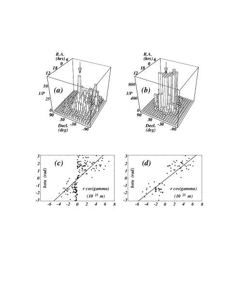
FIG. 1.: Inverse P–values versus anisotropy direction $\vec{s}$, given in terms of its declination and right ascension. $P$ is the fraction of galaxy sets with randomized major axis $(\psi_{\text{rand}})$ and polarization $(\chi_{\text{rand}})$ angles that yielded a linear correlation coefficient $R_{\text{rand}}$ of the set [$r_{i}\cos\gamma_{i},\beta_{i}(\psi_{\text{rand}},\chi_{\text{rand}})$] greater than or equal to the linear correlation coefficient $R_{\text{data}}$ of the original set [$r_{i}\cos\gamma_{i},\beta_{i}(\psi,\chi)$]. (a) All data (160 galaxies). (b) All data with redshift $z\geq 0.3$ (71 galaxies). The figures support an anisotropy direction in the region $\vec{s}^{*}=(\text{Decl.},\text{R.A.})^{*}_{s}=(0^{\circ}\pm 20^{\circ},21\mbox{hrs}\pm 2\mbox{hrs})$. (c) Scatter plot of $\beta$ versus $r\cos\gamma$ for the $\vec{s}$–direction yielding the highest peak (arrow) of (a) for all data. (d) Scatter plot of $\beta$ versus $r\cos\gamma$ for the $\vec{s}$–direction yielding a typical central peak (arrow) of (b) for the cut $z\geq 0.3$.

These studies use the correlation coefficient $R$ appropriate to test unconstrained linear fits of the form $\beta=\frac{1}{2}\Lambda_{s}^{-1}r\cos(\gamma)+\delta$, where $\Lambda_{s}$ and $\delta$ are free parameters. We found that $\delta$ is consistent with zero $(\delta\leq 2^{\circ}$, with $\delta$ typically $\approx 1^{\circ}$) in the region of good correlation ($z\geq 0.3,\;P^{-1}\geq 1000$ or $z\geq 0,\;P^{-1}\geq 25$). We also repeated the entire study using $R=\sum x_{i}y_{i}/(\sum x_{i}^{2}\sum y_{i}^{2})^{1/2}$, which tests the hypothesis of linear correlation with the constraint $\delta=0$, without finding significant changes.

Another study (procedure 2) used a different order. For each random data set (again, galaxy positions were not randomized, as explained above), we varied $\vec{s}$ over the sphere (410 directions) to maximize $R_{\text{rand}}$. This “largest–$R_{\text{rand}}$” value was then recorded. A new random set was then generated, producing another “largest–$R_{\text{rand}}$.” This calculation was repeated more than 1000 times, to create a set of largest $R_{\text{rand}}$’s. This procedure was motivated by the fact that there is an increased probability in procedure 1 of obtaining a fit of $\vec{s}$ to the data due to the two degrees of freedom of $\vec{s}$. The crucial test is for the far–half data set with $z\geq 0.3$, which had a P–value of order $10^{-3}$ (in procedure 1). For the far–half sample with $z\geq 0.3$, we found that the fraction of the largest–$R_{\text{rand}}$’s that exceeded $R_{\text{data}(z\geq 0.3,\vec{s}=\vec{s}^{*})}$ was less than 0.006. The distribution of largest–$R_{\text{rand}}$’s was characterized by a $\sigma$ and $\mu$ such that $R_{\text{data}}=\mu+2.8\sigma$. In contrast, for the closest half of the data, $z<0.3$, the fraction of the largest $R_{\text{rand}}$ exceeding $R_{\text{data}(z<0.3,\vec{s}=\vec{s}^{*})}$ was 0.86, confirming that the effect “turns on” only for the most distant half of the galaxies. We found no instances of largest–$R_{\text{rand}}$’s for the sample with $z<0.3$ exceeding $R_{\text{data}(z\geq 0.3,\vec{s}=\vec{s}^{*})}$. These results provide a more stringent test and corroborate the conclusion of procedure 1. (The authors welcome requests for additional information.)

The average (procedure 1) best fit value is $\Lambda_{s}=(1.1\pm 0.08)10^{25}\frac{h_{0}}{h}\mbox{m}$ for a $\vec{s}$–direction of $(\text{Decl.},\text{R.A.})^{*}_{s}=(0^{\circ}\pm 20^{\circ},21\mbox{hrs}\pm 2\mbox{hrs})$ for the data with $z\geq 0.3$. For the full data set of all 160 data points, we find $\Lambda_{s}=(0.89\pm 0.12)10^{25}\frac{h_{0}}{h}\mbox{m}$ for $(\text{Decl.},\text{R.A.})=(-10^{\circ}\pm 20^{\circ},20\mbox{hrs}\pm 2\mbox{hrs})$. The scale $\Lambda_{s}$, approaching a billion parsecs, is approximately an order of magnitude larger than the largest scales observed in galaxy correlations. (Errors in $\Lambda_{s}$ are the usual 1 sigma variation of uncorrelated analysis and do not refer to probabilities.) The direction $\vec{s}^{*}$ appears unremarkable; although vaguely toward the galaxy center, the cluster in Fig. 1(b) is separated from the galaxy center by $30^{\circ}$, about 30 times the apparent size of the core region of the Milky Way.

As a consistency check, we have separately investigated whether there are strong correlations in $\beta=\Lambda_{s}^{-1}r$, and $\beta=\beta_{0}\cos(\gamma)$. We find nothing significant in the first case, or for the second case over the full data set. The set $z\geq 0.3$ does produce correlations with $\beta_{0}\cos(\gamma)$ which we cannot readily distinguish from Eq. (1), since the $r$–values do not vary enough.

As for conventional physics, the effect observed is not explained by variations on Faraday physics. While fits to Faraday rotation (linear in $\lambda^{2}$) represent a model and an approximation, the ratios of the radio frequency to cyclotron and plasma frequencies are such that the approximation is thought to have exceedingly small corrections. Observers also make corrections for systematic errors and take into account the effects of the Earth’s ionosphere. Consulting with the original observers [4] does not yield any suggestions for bias that would imitate the signal we observe. We have nevertheless questioned whether a local effect of the galaxy, via some unanticipated conventional physics, might account for our correlation. The fact that the correlation is seen for $z\geq 0.3$, but not $z<0.3$, rules out a local effect. (Several observational groups contributed to the $z\geq 0.3$ data, closing the loophole that one particular analysis might contain bias, as best we can determine.) Again, strong fields at the source might generate unexpected initial polarization orientations, or upset the Faraday–based fits, and this could plausibly depend on $z$. But since the correlation is observed in $\cos(\gamma)$, any population–based explanation requires an unnatural, if not impossible, conspiracy between distant sources at widely separated zenith angles. One is left, then, with the option of unknown systematic bias for the large–$z$ set, or accepting the possibility that the correlation is a real physical effect. For the latter, one must arbitrarily invoke coherence on outrageously vast distances, perhaps organized by electromagnetic or other interactions in the early universe, or contemplate new physics.

If we take the data at face value as indicating a fundamental feature of electrodynamics, gauge invariance severely limits the possible couplings of the vector potential $A^{\mu}$ and the electromagnetic field strength tensor $F^{\mu\nu}=\partial^{\mu}A^{\nu}-\partial^{\nu}A^{\mu}$ to any background vector $s^{\mu}$. The unique derivative expansion (units are $\hbar=c=1$) for terms in the effective action $S_{eff}$ is

$$S_{eff}=\int d^{4}x\biggl{(}-{1\over 4}F_{\mu\nu}F^{\mu\nu}+{1\over 4}\Lambda^{-1}_{s}\varepsilon^{\mu\nu\alpha\beta}F_{\mu\nu}A_{\alpha}s_{\beta}\biggr{)},$$ (3)

suppressing higher derivative terms which would contribute to short–distance effects. The dispersion relation for this theory at lowest order in $\Lambda_{s}^{-1}$ is $k_{\pm}=\omega\pm\frac{1}{2}\Lambda_{s}^{-1}\cos(\gamma)$, where $s^{\mu}=(0,\vec{s})$ in the coordinate system where $\omega$ and $k$ are measured. Rotation of the plane of polarization comes from differences in propagation speed between the two modes; the difference $\frac{1}{2}(k_{+}-k_{-})=d\beta/dr$ is a measure of the polarization plane rotation $\beta$ per unit path length $r$, yielding a rotation $\beta$ coinciding with Eq. (1).

The interpretation of the parameters $s^{\mu}$ depends on their physical origin and their transformation properties. If $s^{\mu}$ is odd under time reversal, and its space part is a pseudovector under parity, then Eq. (3) preserves these symmetries separately. If $s^{\mu}$ is also spacelike, as we have assumed, one might associate the vector $\vec{s}$ with an intrinsic “spin axis” of an anisotropic universe. Terms of order $s^{0}$ are dropped consistently if our reference frame coincides well enough with a rest frame of $s^{\mu}$; $s^{0}$ can also be added as a separate parameter. Because the new terms have one less derivative than the standard ones, these terms have no effect (by power counting) on high energy questions such as renormalizability. The scale $\Lambda_{s}$ represents a fundamental length scale in the modified electrodynamics due to Eq. (3), and should not be confused with a “photon mass”, which violates gauge invariance. By converting the length $\Lambda_{s}$ to a mass scale $\mu c^{2}=\Lambda_{s}^{-1}\hbar c$, a value of $\mu=10^{-32}\mbox{eV}/c^{2}$ is found, which is $10^{14}$ times smaller than the photon mass limit of Chibisov, and $10^{17}$ times smaller than Goldhaber and Nieto’s [5].

Ni [6] obtained (3) from covariance arguments; independently it was found from quantum adiabatic arguments (Ralston [6]). The latter was our initial motivation, used to predict the correlation (1), which led to this investigation. The curious history came to light much later. If $s^{\mu}$ is treated as dependent on $x$, then it must be a gradient: $\Lambda_{s}^{-1}s^{\mu}=\frac{g}{8}\partial^{\mu}\phi$, where $g$ is a coupling. The theory is then related to axions [7] or similar pseudoscalar fields $\phi$ with coupling $g$. If a new field is proposed, there should be further observational consequences. Our study of a spacelike $s^{\mu}$ is unconventional compared to other work [2], but there is every reason to think that the observed correlation can be consistent with axion-type domain walls [7], or other condensate structures. More data on the observables is needed, especially from the southern sky. The crucial issues of conventional explanations and experimental systematics merit scrutiny from a broad community. From a scientific standpoint, we report what we find, given the data that exist. We find that the data contain a correlation indicating cosmological anisotropy in electromagnetic propagation. Further study may be able to determine whether (3) or its counterparts invoking new fields might be a valid description of electromagnetism on the largest scale.

B. Anthony-Twarog, K. Ashman, C. Bird, H. Rubinstein, B. Cox, and an anonymous referee made helpful suggestions. DOE Grant Number DE-FG02-85ER40214, NSF Grant Number PHY94-15583, and the $K^{*}STAR$ program provided support.

REFERENCES

- [1] F. F. Gardner and J. B. Whiteoak, Nature 197, 1162 (1963); Ann. Rev. Astr. Astrophys. 4, 245 (1966); G. Burbidge and A. H. Crowne, Astrophys. J. Suppl 40, 583 (1979); H. Spinrad et al., Pub. Astron. Soc. Pacific 97, 932 (1985); J. N. Clarke et al., Mon. Not. R. Astron. Soc. 190, 205 (1980); H. Alven and K. Herlofson, Phys. Rev. 78, 616 (1950).
- [2] S. M. Carroll, G. B. Field and R. Jackiw, Phys. Rev. D 41, 1231 (1990); D. Harari and P. Sikivie, Phys. Lett. B 289, 67 (1992).
- [3] P. Birch, Nature (London) 298, 451 (1982); ibid. 301, 737 (1983); D. Kendall and G. A. Young, Mon. Not. R. Astron. Soc. 207, 637 (1984); M. Bietenholz and P. Kronberg, Astrophys. J. L1, 287 (1984); M. Bietenholz, Astron. J. 91, 1249 (1986).
- [4] P. Kronberg, private communication.
- [5] A. S. Goldhaber and M. M. Nieto, Rev. Mod. Phys. 43, 277 (1971); M. M. Nieto and A. Kostelecky, Phys. Lett. B317, 223 (1993); G. V. Chibisov, Sov. Phys. Usp. 19, 624 (1976).
- [6] W.-T. Ni, Phys. Rev. Lett. 38, 301 (1977); C. Wolf, Phys. Lett. A 132, 151 (1988); ibid 145, 413 (1990); J. P. Ralston, Phys. Rev. D 51, 2018 (1995).
- [7] R. D. Peccei and H. Quinn, Phys. Rev. Lett. 38, 1440 (1977); S. Weinberg, Phys. Rev. Lett. 40, 223 (1978); F. Wilczek, Phys. Rev. Lett. 40, 279 (1978); P. Sikivie, Phys. Lett. B 137, 353 (1984).