ON THE KINEMATICS OF THE DAMPED Ly$\alpha$  PROTOGALAXIES

Abstract

We present the first results of an ongoing program to investigate the kinematic properties of high redshift damped Ly$\alpha$ systems. Because damped Ly$\alpha$ systems are widely believed to be the progenitors of current massive galaxies, an analysis of their kinematics allows a direct test of galaxy formation scenarios. Specifically, the kinematic history of protogalactic gas is a sensitive discriminator among competing theories of galaxy formation.

We use the HIRES echelle spectrograph on the Keck 10 m telescope to obtain accurate, high-resolution spectra of 17 damped Ly$\alpha$ systems. We focus on unsaturated, low-ion transitions such as Si II 1808, since these accurately trace the velocity fields of the neutral gas dominating the baryonic content of the damped systems. The velocity profiles: (1) comprise multiple narrow components; (2) are asymmetric in that the component with strongest absorption tends to lie at one edge of the profile; and (3) exhibit a nearly uniform distribution of velocity widths between 20 and 200 km s^-1 .

In order to explain these characteristics, we consider several physical models proposed to explain the damped Ly$\alpha$ phenomenon, including rapidly rotating “cold” disks, slowly rotating “hot” disks, massive isothermal halos, and a hydrodynamic spherical accretion model. Using standard Monte Carlo techniques, we run sightlines through these model systems to derive simulated low-ion profiles. We develop four test statistics that focus on the symmetry and velocity widths of the profiles to distinguish among the models. Comparing the distributions of test statistics from the simulated profiles with those calculated from the observed profiles, we determine that the models in which the damped Ly$\alpha$ gas is distributed in galactic halos and in spherically infalling gas, are ruled out at more than 99.9$\%$ confidence. A model in which dwarf galaxies are simulated by slowly rotating “hot” disks is ruled out at 97$\%$ confidence. More important, we demonstrate that the Cold Dark Matter Model, as developed by Kauffmann (1996), is inconsistent with the damped Ly$\alpha$ data at more than the 99.9$\%$ confidence level. This is because the CDM Model predicts the interception cross-section of damped Ly$\alpha$ systems to be dominated by systems with rotation speeds too slow to be compatible with the data. This is an important result, because slow rotation speeds are generic traits of protogalaxies in most hierarchical cosmologies.

We find that models with disks that rotate rapidly and are thick are the only tested models consistent with the data at high confidence levels. A Relative Likelihood Ratio Test indicates disks with rotation speeds, $v_{rot}<180$ km s^-1 , and scale heights, $h$ $<$ less than 0.1 times the radial scale length $R_{d}$, are ruled out at the 99$\%$ confidence level. The most likely values of these parameters are $v_{rot}$ = 225 km s^-1 and $h$ = 0.3$R_{d}$. We also find that these disks must be “cold”, since models in which $\sigma_{cc}$/$v_{rot}$ $>$ 0.1 are ruled out with 99$\%$ confidence, where $\sigma_{cc}$ is the velocity dispersion of the gas. We describe an independent test of the “cold” disk hypothesis. The test makes use of the redshift of emission lines sometimes detected in damped Ly$\alpha$ systems, as well as the absorption profiles. The test potentially distinguishes among damped systems that are: (1) large rotating disks detected in absorption and emission, in which case a systematic relation exists between emission redshift and absorption velocity profile, and (2) emitting galaxies surrounded by satellite galaxies detected in damped Ly$\alpha$ absorption, in which case the relation between emission and absorption redshifts is random.

Finally we emphasize a dilemma stimulated by our findings. Specifically, while the kinematics of the damped Ly$\alpha$ systems strongly favor a “cold” disk-like configuration, the low metallicities and type II Sn abundance patterns of damped Ly$\alpha$ systems argue for a “hot” halo-like configuration. We speculate on how this dilemma might be resolved.

keywords cosmology—galaxies: evolution—galaxies: quasars—absorption lines

1 INTRODUCTION

Velocity fields within protogalaxies carry important clues about the process of galaxy formation. The kinematic history of the protogalactic gas is of particular importance as it is a sensitive discriminator between competing theories of galaxy formation. In standard hierarchical models, low-mass subunits of dark matter and gas continuously merge to form the high-mass galaxies seen today [White & Frenk 1991]. In this scenario, the rotation speeds of galaxy disks at high redshifts ($z\gtrsim 2.5$) are low compared to the rotation speeds of current massive spirals [Kauffmann 1996]. By contrast, higher rotation speeds are predicted at large redshifts by models in which disks form from the coherent collapse of gas in massive dark-matter halos [Eggen, Lynden-Bell, & Sandage 1962, Fall & Efstathiou 1980].

The purpose of this paper is to test these ideas directly with data that accurately measure the motions of protogalactic gas. Specifically, we present an analysis of high-resolution spectra of metal absorption lines from a sample of damped Ly$\alpha$ systems. The latter are high-redshift layers of neutral gas widely thought to be the progenitors of current galaxies [Wolfe 1995, Peebles 1993, White & Frenk 1991, Fukugita et al. 1996]. We use the HIRES Echelle spectrograph [Vogt 1992] on the Keck 10 m telescope to detect the gas in absorption against the light of more distant QSOs. The velocity profiles of the damped systems are notable for the following properties: (1) they comprise multiple narrow components; (2) they are asymmetric in that the component with strongest absorption tends to be at one edge of the profile; and (3) the velocity intervals over which absorption occurs, $\Delta v$, are uniformly distributed between $\approx$ 20 and 200 km s^-1 . By constructing statistical measures characterizing the velocity structure of the absorption profiles, we demonstrate that the asymmetry rules out models dominated by random motions or by spherically symmetric radial motions. Rather, we show the asymmetry can be caused by the rotation of “cold” gaseous disks with significant vertical scale heights. Furthermore, the distribution of velocity intervals implies high rotation speeds, $v_{rot}$ $\approx$ 225 km s^-1 .

Two types of models have been proposed to explain the damped Ly$\alpha$ systems. The hierarchical schemes assume the damped systems to be slowly rotating disks embedded in low-mass protogalaxies [Klypin et al. 1995, Mo & Miralda-Escud$\rm\acute{e}$ 1994, Ma and Bertschinger 1994, Kauffmann 1996]. Other models, that do not assume a particular cosmological context, propose the damped systems to be rapidly rotating disks in high-mass protogalaxies [Schiano et al. 1990], protospheroidal gas [Lu et al.  1996b], dwarf galaxies, [York et al. 1986], or gas falling into protogalaxies [Arons 1972]. We compare all the model predictions with the data using Monte Carlo techniques. The models are constructed by inserting gas into discrete velocity components according to algorithms described below. We randomly select the locations and velocities of components along the line of sight from parent distributions appropriate for the scenario being tested. Synthetic spectra are generated by computing the absorption profiles for optically thin transitions arising in low ions such as Si⁺, because the latter accurately traces the velocity structure of the neutral gas. We generate an ensemble of velocity profiles by assuming the model protogalaxies are randomly oriented in projection on the sky. We then compare the computed and observed distributions of statistical measures that are sensitive to the degree of asymmetry and width of the absorption profiles. As demonstrated below, the asymmetry in the velocity profiles rules out “hot” models in which $\sigma_{cc}$ $\gtrsim$ $v_{rot}$ at high confidence levels, where $\sigma_{cc}$ is the component-component velocity dispersion. This is why models with significant random motions are unlikely. We then focus on “cold” rotating disks in which $\sigma_{cc}$ $<<$ $v_{rot}$ and compare the model distribution of $\Delta v$ with the observed distribution. This particular test is crucial for evaluating model disks with different rotation speeds and is the test that rules out models with low $v_{rot}$. In fact, the principal conclusions of this paper is that low rotation speeds, characterizing the bulk of protogalactic disks, in most hierarchical cosmologies, are ruled out at high confidence levels. Rather, protogalactic disks appear to rotate rapidly.

The paper is organized as follows. In $\S$ 2 we discuss the criteria used to select metal-line absorption profiles suitable for model testing. We select a sample of low-ion profiles from 17 damped Ly$\alpha$ systems. Optical depth spectra are constructed that will be used for tests discussed in the following sections. In $\S$ 3 we introduce the rotating disk model and discuss the Monte Carlo methods. Here we determine input parameters used to generate the simulated spectra. We discuss extrinsic parameters such as the number of velocity components, the velocity and position of each component, $\sigma_{cc}$, etc. We also discuss the selection of intrinsic parameters such as the internal velocity dispersion, the column density per component, etc. Together with various model assumptions the parameters are used to create simulated spectra with the noise and spectral resolution of the data. The isothermal halo, spherical infall and random models are discussed in $\S$ 4. The statistical tests are described in $\S$ 5 where attention is given to statistical measures devised to discriminate among the models. In $\S$ 6 we present the results of these tests, in particular demonstrating the failure of all of the models except the “cold”, rapidly rotating disk model. We explore the allowed parameter space for the latter model in $\S$ 7 and perform the Likelihood Ratio Test to determine the most likely set of values for $v_{rot}$ and the thickness of the disks. An independent test of the rotating disk hypothesis is presented in $\S$ 8. Concluding remarks are made in $\S$ 9.

2 PROFILE SELECTION

This section discusses the sample of spectra used for model testing. We construct apparent optical-depth spectra and apply various criteria to them in order to select transitions suitable for testing.

2.1 Data

The data analyzed in this paper were acquired with the High Resolution Spectrograph (HIRES) located at the Nasmyth focus of the 10m W. M. Keck Telescope [Vogt 1992]. Table 1 lists the coordinate name of the background QSO, observation date, exposure time, emission redshift, resolution and signal to noise ratio (SNR) of the damped Ly$\alpha$ systems comprising two data sets. The first data set (W) comprises observations performed by one of us (AMW) as part of a long term project to measure the metallicity and kinematics of damped Ly$\alpha$ systems. With the exception of Q1331+170, the C5 decker, that has a FWHM resolution of $\approx$ 8 km s^-1 , was used for all of the observations. For Q1331, we used the C1 decker that gives a higher FWHM resolution of $\approx 6$ km s^-1 . The latter resolution and setup was used by W. L. W. Sargent who generously provided the second data set (S).

Table 1: QSO AND OBSERVATIONAL DATA

QSO	Date	Exposure	$z_{em}$	Resolution	SNR	Data
		Time (s)		(km s-1 )		set
Q0100+1300	S94	11700	2.69	7.5	40	W
Q0201+3634	F94	34580	2.49	7.5	35	W
Q0458$-$0203	F95	28800	2.29	7.5	15	W
Q1215+3322	S94	14040	2.61	7.5	20	W
Q1331+1704	S94	36000	2.08	6.6	80	W
Q2206$-$1958A,B	F94	25900	2.56	7.5	40	W
Q2231$-$0015	F95	14400	3.02	7.5	30	W
Q0216+0803	F94,F95	18600	2.992	6.6	24	Sa
Q0449$-$1325	F94	16000	3.097	6.6	40	S
Q0528$-$2505b	F94,S95	24000	2.779	6.6	25	S
Q1202$-$0725	S95	33000	4.7	6.6	30	S
Q1425+6039	S95	37200	3.173	6.6	100	S
Q1946+7658A,B	S94	8700	2.994	6.6	55	S
Q2212$-$1626	F93,F95	33000	3.992	6.6	75	S
Q2237$-$0608	F94, F95	56000	4.559	6.6	22	S

^a Data kindly provided by W. L. W. Sargent and collaborators

^b The $z=2.811$ damped system toward Q0528$-$2505 was omitted because its redshift exceeds that of the background QSO to which it may be associated.

All of the data were reduced with a software package kindly provided by T. Barlow. Briefly, the routine optimally extracts the data from its 2-D CCD format into 1-D spectra by using a bright standard star image as a trace. The package properly flat fields and wavelength calibrates the data with the quartz and ThAr calibration frames while removing cosmic rays. Finally, the data is continuum fitted with the IRAF package continuum. The reduction process is both accurate and relatively free of systematic errors. Thus the data sample is essentially homogeneous with the only variations arising from differences in SNR and resolution. The sample is also unbiased, because the objects were selected without a priori knowledge of the kinematic structure of the absorbing gas. Rather, the objects were selected for: (1) large H I column density $N$(H I) $\geq$ 2$\times$10²⁰ cm^-2, and (2) brightness of the background QSO, $V$ $\leq$ 19.

Figure 1: Velocity profiles of low-ion transitions from 17 damped Ly$\alpha$ systems comprising our empirical sample. For each profile, $v=0$ km s^-1 corresponds to the redshift labeled in the plot.

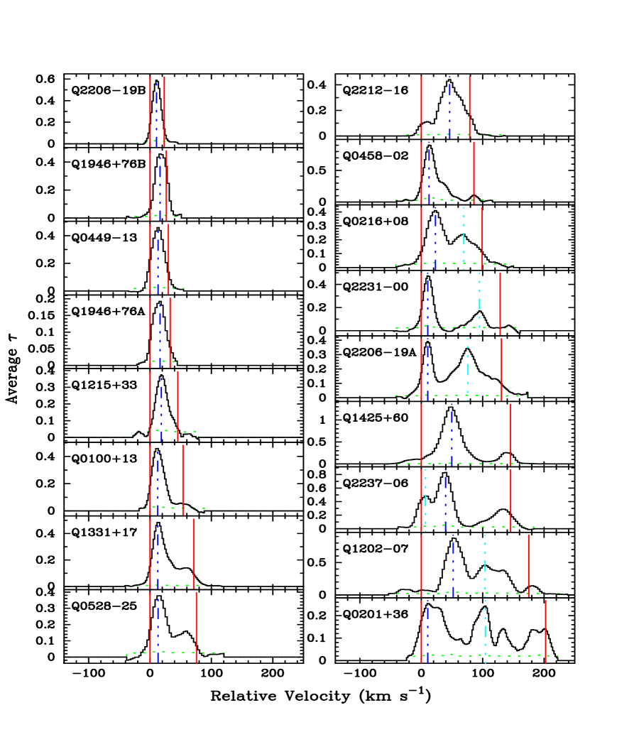
Figure 2: Average optical depth profiles (binned over 9 pixels) for the same 17 transitions presented in Figure 1. The solid vertical lines designate the velocity interval, $\Delta v$, while the dash-dot lines indicate peaks and the dotted line is the $2\sigma(\bar{\tau})$ array. The profiles have been shifted in velocity space such that the left edge of the velocity interval coincides with $v=0$ and reflected if necessary so that the strongest peak always lies on the left edge of the interval.

2.2 Profile Selection Criteria

In order to form an ensemble of velocity profiles we select the profile of a single transition from each damped Ly$\alpha$ system. We first require that the line profile be free from blending with other absorption line profiles. This condition is met by intracomparing a set of three or more transitions from each damped Ly$\alpha$ system. We next construct an apparent optical-depth spectrum,

$$\tau(v)\equiv\ln[I_{c}/I(v)]\;\;\;,$$ (1)

where $I(v)$ and $I_{c}$ are the transmitted and incident intensities at velocity $v$. To focus on spectral features rather than individual pixels, we create a binned optical depth array by averaging $\tau(v)$ over a running window nine pixels wide:

$${\bar{\tau}(v_{i})}={1\over 9}{\sum_{j=i-4}^{i+4}{\tau(v_{j})}}\;\;\;.$$ (2)

In the last equation $\tau(v_{j})$ is the apparent optical depth at the $j^{th}$ velocity pixel and the sum is over the four nearest neighbors of pixel $i$ inclusive.

In order to assure the detection of weaker features, which is crucial for establishing asymmetries in the line profiles, we demand that $\bar{\tau}(v_{pk})$, the $\bar{\tau}(v)$ of the strongest feature (i.e. the feature with peak optical depth), exceed 20$\sigma(\bar{\tau})$ significance. Specifically, with this criterion we can detect features with $\bar{\tau}(v)$ $\geq$ 0.25$\times$$\bar{\tau}(v_{pk})$ at 5$\sigma$ significance. For spectra with SNR $\approx$ 30 this criterion implies the strongest feature must satisfy $I(v_{pk})/I_{c}$ $\leq$ 0.6. Because saturated lines are strongly affected by opacity that can mask asymmetries and component structures detectable in optically thin transitions, we set an upper limit on $\bar{\tau}(v)$ by demanding $I(v_{pk})/I_{c}$ $\geq$ 0.1. Therefore, we require 0.1 $\leq$ $I(v_{pk})/I_{c}$ $\leq$ 0.6 and note the upper limit will vary with SNR. Given a single transition satisfying this criterion, the results are independent of the ionic species or the metallicity of the damped systems, provided the metals trace the HI gas (i.e., the system is well mixed).

Our analysis focuses on low-ion transitions arising in gas giving rise to damped Ly$\alpha$ absorption lines. Ions such as Fe⁺, Si⁺, and Ni⁺ are accurate tracers of neutral hydrogen when $N$(H I) $\geq$ 2$\times$10²⁰ cm^-2, because the optical depth at the Lyman limit, $\tau_{LL}$ $>$ 10³. Moreover, the large ratios of Al⁺/Al⁺⁺ and Si⁺/Si³⁺ demonstrate the gas containing low ions is mainly neutral (Prochaska & Wolfe 1996, 1997). The low-ion transitions selected for analysis are given in column 4 in Table 2. The table also gives the QSO name in column 1, the absorption redshift in column 2, the H I column density in column 3, the ratio $\bar{\tau}(v_{pk})/\sigma(\bar{\tau})$ in column 5, and the reference for each of the 17 systems in column 6. The corresponding intensity profiles are presented in Figure 1. The binned optical-depth spectra constructed from these profiles are shown in Figure 2. If necessary, we reflect the profiles to place the peak component at lower velocities.

Table 2: DAMPED LYMAN ALPHA STATISTICAL SAMPLE

QSO	$z_{abs}$	$\log[{N({\rm HI})}]$	Transition	$\tau_{pk}$/$\sigma_{\tau}$	Ref.
		cm-2
Q0100+1300	2.309	21.4	Ni II 1741	29	1
Q0201+3634	2.462	20.4	Si II 1808	21	2
Q0458$-$0203	2.040	21.7	Cr II 2056	26	$-$
Q1215+3322	1.999	21.0	Si II 1808	20	$-$
Q1331+1704	1.776	21.2	Si II 1808	92	$-$
Q2206$-$1958A	1.920	20.7	Ni II 1741	41	3
Q2206$-$1958B	2.076	20.4	Al II 1670	41	3
Q2231$-$0015	2.066	20.6	Si II 1808	22	4
Q0216+0803	2.293	20.5	Si II 1808	23	4
Q0449$-$1325	1.267	N/A	Fe II 2249	34	4
Q0528$-$2505	2.141	21.0	Si II 1808	22	4
Q1202$-$0725	4.383	20.6	Si II 1304	40	5
Q1425+6039	2.827	20.3	Fe II 1608	90	4
Q1946+7658A	2.843	20.3	Si II 1304	50	4,6
Q1946+7658B	1.738	N/A	Si II 1808	29	4,6
Q2212$-$1626	3.662	20.2	Si II 1304	65	4
Q2237$-$0608	4.080	20.5	Al II 1670	32	4

¹ [Wolfe et al. 1994]

² [Prochaska and Wolfe 1996]

³ [Prochaska and Wolfe 1997]

⁴ [Lu et al.  1996b]

⁵ [Lu et al. 1996a]

⁶ [Lu et al. 1995a]

The spectra in Figures 1 and 2 are notable for several reasons. First, the unbinned spectra in Figure 1 show the profiles comprise multiple, narrow velocity components. Second, the velocity intervals over which absorption occurs are uniformly distributed between $\approx$ 20 and 200 km s^-1 . Third, the velocity profiles in Figure 1 are asymmetric in that the location of the strongest component tends to lie at one edge of the velocity profile in 12 out of 17 cases. Fourth, the binned spectra in Figure 2 show evidence for a monotonic sequence of velocity components in which optical depth decreases with increasing velocity. To be successful, a kinematic model must quantitatively explain these characteristics in a natural way.

3 ROTATING DISK MODELS

Rotating disks have figured prominently in damped Ly$\alpha$ research. The original survey for damped Ly$\alpha$ lines was initiated in order to find rotating galactic disks at high redshifts [Wolfe et al. 1986]. Since then, much of the modeling has incorporated rotating disks as a working hypothesis (e.g., [Schiano et al. 1990, Fall & Pei 1993, Kauffmann 1996]). The first attempt to infer the velocity field of the gas from the data was made by Briggs et al. (1985) who argued the red-blue asymmetry detected in the metal lines of a $z$ $<$ 1 damped absorber could arise from passage of the line of sight through a rotating disk. Working with higher resolution data Lanzetta & Bowen (1992) presented formulae for velocity profiles arising from highly inclined sightlines through a rotating spheroid, that mimic sightlines through a thin rotating disk, in order to model the asymmetries they found in three damped systems with $z$ $<$ 1. Using even more accurate HIRES spectra Wolfe (1995) noticed similar asymmetries in the metal-line profiles of five damped systems with $z$ $>$ 1.7. Wolfe (1995) assumed the velocity profiles arose in rotating disks of gas in which the gas distribution decreases exponentially both with radius and vertical distance from the plane. A Monte Carlo approach to this problem was outlined, and a preliminary description of the present work was given in Wolfe (1996).

In $\S 6$ the techniques described in this section will be applied to: (1) rapidly rotating “cold” disks of massive galaxies; (2) slowly rotating “hot” disks of dwarf galaxies; and (3) rotating disk progenitors of ordinary spirals predicted by the CDM cosmology.

3.1 Kinematic Model

Assume the velocity profiles in damped Ly$\alpha$ systems are explained by passage of the line of sight through a centrifugally supported disk in which the volume density of neutral gas is given by

$$n(R,Z)=n_{0}\exp\left[\,-{R\over R_{d}}-{|Z|\over h}\,\right]\;\;\;,$$ (3)

where $R$ and $Z$ are cylindrical radius and vertical displacement from midplane, $n_{0}$ is the central gas density, $R_{d}$ is the radial scale length, and $h$ is the vertical scale height. The column density of gas perpendicular to the disk is thus

$$N_{\perp}(R)=N_{\perp}(0)\exp\left(\,-R/R_{d}\,\right)\;\;\;,$$ (4)

where the central perpendicular column density,

$$N_{\perp}(0)=2n_{0}h.$$ (5)

Because the velocity profiles in Figure 1 indicate the density field comprises a discrete rather than continuous distribution of gas in velocity space, $n(R,Z)$ is proportional to the number of discrete clouds (i.e., velocity components) per unit volume, if, as we assume, the column density per cloud remains constant. Further suppose the gas rotates with a flat rotation curve given by

$$v_{\phi}(R,Z)=v_{rot},$$ (6)

where $v_{\phi}$ is the azimuthal component of the velocity. Although equation 6 breaks down at values of $Z$ where the $R^{th}$ component of the gravitational force differs significantly from its value at $Z$ = 0, we shall assume this equality is valid at all $Z$, and re-examine this assumption in $\S$ 9. In addition, let the clouds exhibit isotropic random motions characterized by a one-dimensional velocity dispersion, $\sigma_{cc}$.

The profile asymmetry is the product of two effects. The “radial effect” stems from the $R$ dependence of $n(R,Z)$ along the line of sight. This produces a cloud distribution symmetric about the peak located where $R$ equals the impact parameter, $b$, i.e., where the sightline crosses the major axis of the inclined disk (see Figure 3 where the major axis is denoted by the horizontal dash-dot line and the line of sight by the vertical dashed line). In this case the strongest absorption occurs at the smallest value of $R$ where the magnitude of the rotational velocity projected along the line of sight is largest; i.e., the “tangent point” used in 21 cm investigations of the Galactic rotation curve [Mihalas and Binney 1981]. As $R$ increases, the absorption gets weaker and the magnitude of the projected rotational velocity decreases, thereby producing a velocity profile with strong absorption at one side of the profile and progressively weaker absorption toward the other. The “perpendicular effect” stems from the $Z$ dependence of $n(R,Z)$ along the line of sight. If the line of sight intersects midplane, $Z$ = 0, more than a few scale heights from the major axis, the cloud distribution will peak at the intersection point rather than the major axis, because $h$ $<$ $R_{d}$. The resultant cloud distribution along the line of sight is lopsided with more clouds expected toward than away from the major axis, owing to the “radial effect”. The asymmetry of this profile is the reverse of the previous profile, because the absorption is strongest where the magnitude of $v_{rot}$ projected along the line of sight is smallest and weakens as the magnitude of this velocity component increases toward the major axis.

Figure 3 shows examples of velocity profiles arising from these effects. The profiles designated 1 and 2 are caused by sightlines intersecting midplane at locations 1 and 2. The profiles are produced by absorption in discrete clouds and are computed according to the prescription given in the next subsection. The asymmetry of profile 2 is dominated by the radial effect because the midplane intersection is so close to the major axis. Profile 1 exhibits the reverse asymmetry because the midplane intersection is so far from the major axis. Figure 3 also shows how the velocity profiles are affected by changes in $b$. Profiles 3$-$5 arise at midplane intersections with increasing $b$ which are displaced from the major axis by the same distance along the line of sight. The absorption intervals, $\Delta v$, decrease with increasing $b$, because the gradient of $v_{rot}$ projected along the line of sight decreases with increasing $R$.

Figure 3: The center circle represents an inclined disk (top view) rotating counter clockwise with rotation speed $v_{rot}=250$ km s^-1 . The solid dots represent the intersection points for 5 different sightlines with the midplane of the disk. The solid arrows indicate the direction of the rotation vector. The dashed vertical line represents the sightline for intersections 1 and 2. Finally, the dash-dot line is the kinematic major axis, i.e. the intersection of the plane of the disk and the plane of the sky. The sightlines are inclined by 70 $\deg$ with respect to the normal of the disk and yield the profiles labeled 1$-$5. See the text for a discussion of the profiles.

3.2 Monte Carlo Methods

To generate a statistical ensemble of velocity profiles we adopt a Monte Carlo technique in which sightlines penetrate the midplanes of randomly oriented disks at random locations. The clouds responsible for absorption are randomly selected from the $n(R,Z)$ distribution constrained at fixed impact parameter, $b$ = $R$cos$\phi$, where $\phi$ is the azimuthal angle in the plane of the disk. More specifically, we use the following prescription:

(1) Pick input parameters $N_{\perp}(0)$, $N_{c}$, $\sigma_{int}$, $h/R_{d}$, $\sigma_{cc}$, and $v_{rot}$, where $N_{c}$ is the H I column density per cloud, and $\sigma_{int}$ is the velocity dispersion internal to a cloud. For all our disk models we let $\sigma_{int}$ = 4.3 km s^-1 . The value of $\sigma_{int}$ approximates the internal velocity dispersions of Gaussian velocity components used to model velocity profiles in damped systems [Wolfe et al. 1994, Prochaska and Wolfe 1996, Prochaska and Wolfe 1997]. Because the velocity profiles do not depend on an absolute length, we express all length scales in units of $R_{d}$. The remaining parameters either remain fixed during the simulation of a given ensemble of velocity profiles, i.e, during one run, or vary from one profile to the next.

(2) Randomly select the angle of inclination $i$ of the disk, where $i$ is the angle between the normal to the disk and the line of sight.

(3) Randomly draw coordinates of the midplane intersection, ($X,Y$), from the uniform projection of the inclined disk onto the plane of the sky, i.e., onto the ellipse

$${X^{2}\over R_{f}^{2}}+{Y^{2}\over R_{f}^{2}\cos^{2}i}\leq 1\;\;\;,$$ (7)

where the $X$ axis coincides with the major axis of the inclined disk. We set $R_{f}$ to be sufficiently large that sightlines outside the ellipse will not encounter ${N({\rm{\rm HI}})}\geq 2{\rm\;\times\;10^{20}}\,\rm cm^{-2}$. For the values of $N_{\perp}(0)$ adopted here, we find that $R_{f}\approx 10\,R_{d}$ is satisfactory. Given the midplane intersection and inclination angle, the line of sight is uniquely defined by setting $X$ equal to the impact parameter, $b$.

(4) Compute $N(X,Y)$, the H I column density along the line of sight, from the integral $\int\limits_{X=b}n(R,Z)ds$ where $ds$ is the differential length element along the line of sight and $R$ = $R(s)$ and $Z$ = $Z(s)$.

(5) Choose a minimum value for $n_{c}$ at the ${N({\rm HI})}$ threshold (see below) and then for columns above threshold let $n_{c}$ be proportional to $N(X,Y)$. After $n_{c}$ is selected, pick clouds randomly along the line of sight according to the distribution $n(R,Z)$.

(6) Determine the ionic column density and oscillator strength, $f$, that gives rise to the synthetic profile for the adopted transition with wavelength $\lambda$. We assume $\lambda=1808.0126{\rm\,\AA}$, the wavelength of the Si II 1808 resonance transition, $10^{12.5}\,\rm cm^{-2}$ for the ionic column density of each cloud, and normalize $f$ such that the product of $N_{c}f\lambda$ produces a line profile that satisfies the line selection criteria, i.e. having the observed $\bar{\tau}(v_{pk})/\sigma(\bar{\tau})$. Therefore, the choice of $N_{c}$ and $\lambda$ are arbitrary.

(7) Compute the simulated profile by (a) solving the transfer equation for the cloud ensemble, (b) smoothing the spectrum to the instrumental resolution of HIRES, and (c) adding Gaussian noise such that the SNR of the synthetic profiles corresponds to each of the 17 observed profiles in Figure 1. Repeat this procedure 500 times for each observed profile in order to compute 8,500 synthetic velocity profiles for a given run.

Let us discuss the input parameters in more detail. The profiles are obviously sensitive to $v_{rot}$, $h/R_{d}$, and $\sigma_{cc}$/$v_{rot}$. In the limit $\sigma_{cc}\ll v_{rot}$, the velocity widths are mainly affected by $v_{rot}$ and $h/R_{d}$, because $\Delta v$ $\propto$ $v_{rot}$ and a fixed length of sightline samples an increasing fraction of the rotation curve as $h/R_{d}$ increases. The symmetry of the profiles is affected by $\sigma_{cc}/v_{rot}$ and $h/R_{d}$, because the systematic nature of the velocity field is diluted as the contribution made by random motions increases and because small values of $h/R_{d}$ result in narrow symmetric profiles. The profiles are indirectly sensitive to $N_{\perp}(0)$. The portion of the disk selected for the statistical sample lies within the elliptical contour defined by $N(X,Y)$ $\geq$ 2$\times$10²⁰ cm^-2, hence the quantity $N_{\perp}(0)$ determines the size of the “available” disk. If $N_{\perp}(0)$ is large, the “available” disk extends out to many radial scalelengths, $R_{d}$. In that case the impact parameter to a typical sightline will be large compared to $R_{d}$. This produces a small gradient in $v_{rot}$ projected along the line of sight, that results in profiles with small $\Delta v$ (see sightlines 3$-$5 in Figure 3). Conversely when $N_{\perp}(0)$ is small, larger $\Delta v$ will be typical. We shall refer to this effect as the “column-density kinematic effect”. In order to reproduce the observed distribution of H I column densities, we selected $N_{\perp}(0)$ with values between 10^20.8 and 10^21.6 cm^-2.

Figure 4: Comparison of two line-profile fits to (a) the Si II 1808 transition from the $z=1.776$ damped system toward Q1331$+$170 and (b) the Cr II 2056 transition from the $z=2.040$ system toward Q0458$-$020. In both figures, the dotted histogram is the observed profile, the solid lines represent the individual components of the VPFIT solution, and the dash-dot line is the convolved final solution. Note that even though profile (a) has a smaller $\Delta v$ than that of the Q0458 profile, the VPFIT solution required 2 more clouds than the lower SNR Q0458 data.

On the other hand the velocity profiles are much less sensitive to $n_{c}$, the number of clouds along the line of sight, provided $v_{rot}$ $>>$ $\sigma_{cc}$; i.e., when the kinematics are dominated by systematic rather than random motions. The decomposition of the absorbing gas into multiple discrete clouds is based on our experience with fitting model profiles to the high-resolution HIRES spectra (see [Wolfe et al. 1994, Prochaska and Wolfe 1996, Prochaska and Wolfe 1997]). Using chi square fitting techniques we find that $\approx$ five Gaussian velocity components are the minimum number necessary for acceptable fits, with no strict upper limit. That is, we find trials with $n_{c}=60$ yield test statistics ($\S$ 5) similar to those trials with $n_{c}\approx 5$. Although the narrowest 4 profiles in the observed data set can be modeled with only 1 or 2 components, these features are probably blends of a greater number ($>5$) of components superimposed in velocity space. The case for large numbers of components is supported by the fact that when $\Delta v$ is fixed, $n_{c}$ increases with increasing SNR. In Figure 4 we show our model fits to (a) the Si II 1808 profile for the $z=1.776$ damped system toward Q1331$+$170 and (b) the Cr II 2056 profile for the $z=2.040$ system toward Q0458$-$020. Although $\Delta v$ for the Q1331 profile is below the mean for the sample, our best solution requires $n_{c}=7$. By contrast we need only 5 components to fit the wider, but noisier Cr II profile from the $z=2.04$ damped system toward Q0458$-$020.

Therefore, in each run we adopt $n_{c}$ = 5 for threshold impacts, $N(X,Y)=2{\rm\;\times\;10^{20}}\,\rm cm^{-2}$, and then let $n_{c}$ be proportional to higher values of $N(X,Y)$ for impacts within the threshold ellipse. The crucial point is that the results are insensitive to $n_{c}$ for $n_{c}$ $>$ 5. The minimum value for $n_{c}$ is important, because if it were significantly smaller, velocity asymmetries could arise from strong Poissonian fluctuations in the strengths of the velocity components rather than from gradients in systematic velocity fields. We also find the results discussed below to be insensitive to $\sigma_{int}$, provided it is small compared to $v_{rot}$ or $\sigma_{cc}$.

4 MODELS WITHOUT ROTATING DISKS

We now discuss the kinematic predictions of other models suggested to explain the damped Ly$\alpha$ systems. In particular we consider models in which rotation does not dominate the velocity field. The Monte Carlo methods used for these tests are essentially those presented for the disk model in $\S$ 3.2.

4.1 Isothermal Halos of Normal Galaxies

The low metallicities measured in damped Ly$\alpha$ systems, [Zn/H] $\approx$ $-$1.2 [Pettini et al. 1994], and the pattern of relative metal abundances in these objects [Lu, Sargent, & Barlow 1995, Lu et al.  1996b] bring to mind Galactic halo stars; i.e., stars that were metal enriched only by type II supernovae. For these reasons Lu et al. (1996b) suggest the damped systems comprise neutral clouds in galactic halos. The abundance patterns of damped Ly$\alpha$ systems argue against metal-enriched disks of current spiral galaxies, because metal enrichment by type I as well as type II supernovae are required to explain their abundance patterns. We wish to test the halo hypothesis by modeling the cloud kinematics with an isothermal halo.

To determine the velocity profiles we consider an isothermal halo model in which $n(r)$, the gas density at 3D radius $r$, is proportional to the total mass density $\rho(r)$ given by Table 4-1 in Binney and Tremaine (1987) for self gravitating isothermal spheres. The proportionality constant is fixed by setting the universal baryon to dark matter ratio to 0.1 [Navarro, Frenk & White 1995]. As a result, all the baryonic mass in galaxies is initially placed in the halo. In this model the mass of neutral gas in the halo cannot vary significantly between $z$ $\approx$ 3 and 1.5 in order to explain the relatively constant comoving density of neutral gas observed in this redshift interval [Storrie-Lombardi and Wolfe 1997]. Because halos are dominated by random rather than systematic motions such as rotation, the asymmetries predicted for the “cold” rotating disks should be suppressed in this model, provided significant velocity gaps between the clouds do not exist. This is illustrated in Figure 5 showing eight $\bar{\tau}(v)$ profiles generated by a model of this type.

Figure 5: Average optical depth profiles derived from the isothermal halo model with varying cloud number $n_{c}$ and impact parameter $b$. Note the profiles tend to peak near $v=0$ particularly as $n_{c}$ increases. The profiles also have very large velocity intervals, exceeding 200 km s^-1 in the majority of cases.

4.2 Spherical Accretion onto Galaxy Bulges

The infall of gas onto pre-existing mass concentrations is a plausible scenario for galaxy formation, one that may give rise to the velocity profiles in damped Ly$\alpha$ systems. Such mass concentrations may have recently been discovered in the form of compact galaxy bulges with redshifts of $z\approx$ 3.5 [Steidel et al. 1996]. The regularity of the brightness distributions further suggests these objects formed at even higher redshifts, and reinforces the idea that the remaining parts of the galaxy may have formed by infall of neutral gas onto a pre-existing bulge component [Peebles 1993]. Gaseous infall was first suggested by Arons (1972) who proposed that QSO absorption lines originated in gas partaking in the gravitational collapse of low mass protogalaxies. Because he focused on the highly ionized gas responsible for the low column-density Ly$\alpha$ forest systems, his model is not directly applicable to the neutral gas comprising the damped Ly$\alpha$ systems.

Figure 6: Average optical depth profiles derived from the spherical accretion model with varying cloud number $n_{c}$, impact parameter $b$, and infall velocity $v_{inf}$. Unlike all of the other models considered, these profiles exhibit peaks at both edges of the velocity interval.

We model the infall by assuming neutral clouds responsible for the damped Ly$\alpha$ systems are embedded in a hydrodynamical infall of fluid onto a spherical mass distribution. By assuming spherical symmetry we can adopt the analysis of Bondi (e.g. [Shapiro & Teukolsky 1983]) for hydrodynamical spherical accretion. In this case the radial velocity and volume density of the fluid are given by

$$v(r)=-v_{0}\left(\,{r_{s}\over r}\,\right)^{1\over 2}\;\;\;\;[r\ll r_{s}]\;\;\;,$$ (8)

and

$$n(r)=n_{0}\left(\,{r_{s}\over r}\,\right)^{3\over 2}\;\;\;\;[r\ll r_{s}]\;\;\;,$$ (9)

where $v_{0}$ and $n_{0}$ are the radial velocity and density at $r=r_{s}$. The quantity $r_{s}$ is the transonic radius and is related to the ambient thermal energy per unit mass (i.e., the sound speed squared), $a_{\infty}^{2}$, by

$$r_{s}\approx{GM\over a_{\infty}^{2}}\;\;\;.$$ (10)

In this model the gas has zero net angular momentum; future work will address a scenario with finite net angular momentum.

Figure 6 shows examples of velocity profiles produced by a typical accretion model. Notice the double absorption peaks located at both edges of the profile. These are caused by the maxima in the line-of-sight component of $v(r)$ at displacements $\pm$ $b$ from the point of closest approach. By contrast the profiles produced by “cold” rotating disks tend to produce single peaks at the profile edges (see Figure 3).

4.3 Random Motion Models

In order to generate a control sample, that is, a sample of velocity profiles created by velocity fields without inherent systematics, we investigate a model in which the velocities are randomly drawn from a uniform velocity distribution covering the velocity interval $v$ = [0,$v_{max}$]. The model has a generic problem matching the observations in that it yields nearly the same $\Delta v$ for each simulated line profile. This is in obvious conflict with the observed profiles exhibiting a wide range of $\Delta v$. Because the neutral volume density, $n$, is not described by this model, it does not yield values of $N$(H I). Therefore, for each run we arbitrarily select the number of individual clouds from the interval $n_{c}$ = [5,25], resulting in variations of $N$(H I).

5 STATISTICAL TESTS

Figure 7 is a plot of characteristic line profiles for each of the models for a smooth distribution of gas ($n_{c}\gg 1$). Rapidly rotating disks are characterized by asymmetric distributions in optical depth that tend to peak at one edge of the velocity interval. The spherical accretion model produces peaks at both edges, the random motions model produces a flat profile without peaks, while central peaks or null peaks characterize “hot” models where $\sigma_{cc}$ $\gtrsim$ $v_{rot}$. In this section we design test statistics to discriminate among these models. In particular, the tests focus on the width of the features in velocity space (the velocity interval), the location of the peak component within the velocity interval, and the degree of asymmetry evident in the profiles.

5.1 Velocity Interval Test

The velocity interval, $\Delta v$, of an absorption profile is defined as the width of the profile in velocity space. A simple method for determining $\Delta v$ is to identify the $3\sigma$ components at the lowest and highest velocities of the ${\bar{\tau}(v)}$ array and define $\Delta v$ as the difference in velocity between these components. This approach, however, gives weak outlying components the same weight as strong components in the main absorption complex. As a result a single, weak component displaced 200 km s^-1 from the centroid of a strong absorption complex spanning a velocity interval of 40 km s^-1 would yield $\Delta v\approx$ 220 km s^-1 even though most of the absorption spans a much smaller $\Delta v$.

Figure 7: Smooth absorption profiles for the (a) Thick Rotating Disk (TRD) (b) Spherical Accretion (SPH) (c) Random Motion (RAN) and (d) Dwarf Galaxy (DG). Profiles derived by setting $n_{c}=1000$.

For this reason we define $\Delta v$ as the velocity interval weighted by optical depth. Specifically, define $\Delta v$ by first computing the integrated optical depth

$$\tau_{tot}=\int{\tau(v)}dv\;\;\;.$$ (11)

We then step inward from each edge of the profile until reaching the pixel where 5$\%$ of $\tau_{tot}$ is removed, and set $\Delta v$ equal to the velocity difference between the pixels. This definition removes outlying weak components that may be statistical fluctuations that are not good tracers of the underlying velocity field. While the routine may underestimate the true velocity interval, this is preferable to including misleading statistical artifacts. In addition, numerical tests (see Figure 8) reveal the removal algorithm is not sensitive to the optical depth of the absorption feature. Although the choice of removing $10\%$ of $\tau_{tot}$ is somewhat arbitrary, the simulations indicate the other statistical tests are largely independent of the removed fraction of $\tau_{tot}$.

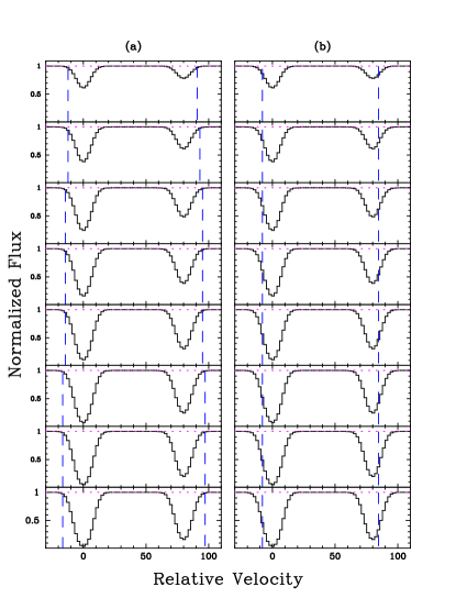
Figure 8: Comparison of the effects of saturation on the definition of the velocity interval by (a) a 3$\sigma$ limit in the $\bar{\tau}(v)$ array and (b) designating 90$\%$ of the total optical depth. Note that the velocity interval for the optical depth method remains constant with increasing line strength, while the velocity interval derived with the 3$\sigma$ limit clearly increases ($\approx 20\%$ from the first to last frames).

5.2 Mean$-$Median Test

One of the principal characteristics of the velocity profiles is their asymmetry, and so we devise a number of test statistics to discriminate asymmetric profiles from symmetric ones. The Mean$-$Median Test gauges asymmetry by measuring the relative difference between the mean and median velocities of the optical depth profile. The test first establishes the velocity interval as discussed above. The mean velocity is defined as the velocity of the midpoint of the interval where the edge corresponding to the smallest velocity is normalized to $v=0$ (i.e. $v_{mean}={1\over 2}\Delta v$). The routine calculates $\tau_{tot}$ within the velocity interval, and then determines the median velocity, $v_{median}$, as the velocity dividing $\tau_{tot}$ in half. The formal statistic is expressed as:

$$f_{mm}={|v_{mean}-v_{median}|\over(\Delta v/2)}\;\;\;.$$ (12)

For a perfectly symmetric distribution of gas, $f_{mm}=0$, while more asymmetric profiles will tend to $f_{mm}=1$. The test is both physically motivated and relatively simple. Note that because the Velocity Interval routine removes $10\%$ of $\tau_{tot}$ symmetrically, it does not affect the Mean$-$Median Test.

5.3 Edge-Leading Test

The test statistic, $f_{edg}$, measures the relative velocity difference between $v_{pk}$, the velocity of the feature with peak ${\bar{\tau}}(v)$, and $v_{mean}$ such that

$$f_{edg}={|v_{pk}-v_{mean}|\over(\Delta v/2)}\;\;\;.$$ (13)

Thus, $f_{edg}$ = 0 for peaks at the center of the profile, while very “edge-leading” profiles yield $f_{edg}\approx 1$.

5.4 Two Peak Test

A third test statistic, designed to accentuate the location of the second strongest peak in the velocity profiles, is given by

$$f_{2pk}={\pm}\frac{|v_{2pk}-v_{mean}|}{(\Delta v/2)},$$ (14)

where $v_{2pk}$ is the velocity of the second strongest peak. The plus sign holds if the second peak is between the velocity of the first peak, $v_{pk}$, and $v_{mean}$, otherwise the negative sign holds. Consequently, profiles with peaks at both edges, as would arise in the case of spherical accretion, or profiles in which $v_{2pk}$ $<$ $v_{pk}$, that might be drawn from Gaussian velocity distributions, can be distinguished from the peaks arising from rotating exponential disks. The disk model tends to produce peaks with $v_{pk}$ $<$ $v_{2pk}$ $<$ $v_{mean}$ because $\tau(v)$ systematically decreases with increasing $v-v_{pk}$. In fact, the Two$-$Peak Test was introduced to differentiate between the rotating disk and spherical infall models. In the random models the two strongest peaks should be uncorrelated and will occur at velocities uniformly distributed within $\Delta v$. While uncorrelated, the two strongest peaks will be more centrally located in models for which $\sigma_{cc}$ $>$ $v_{rot}$, since the random part of the velocities are drawn from a Gaussian rather than a uniform velocity distribution.

As in the Edge-Leading Test, this test first finds the strongest feature in the velocity interval. It then searches across $\Delta v$ for a second significant feature satisfying two criteria: (1) $\bar{\tau}(v_{2pk})>{1\over 3}\bar{\tau}(v_{pk})$; and (2) $\bar{\tau}(v_{2pk})$ is a $3\sigma$ feature above an artificial continuum level set by the lowest $\bar{\tau}(v_{i})$ value reached between $v_{pk}$ and $v_{2pk}$. The first criterion prevents small, physically irrelevant, features from biasing the test. The second criterion is necessary to distinguish a physically distinct second peak from a small rise on a single feature (see Figure 9). After the two peaks are determined, the test measures the relative velocity of the second strongest peak from the center of the velocity interval. Note that if there is no significant second peak, the value for $f_{edg}$ is adopted instead. Therefore, models preferentially yielding profiles with single peaks will have an $f_{2pk}$ distribution biased to positive values.

Figure 9: Average optical-depth profiles for two systems, (a) one exhibiting two peaks and the other (b) only a single peak. The down arrows indicate peaks while the up arrow indicates the boundary between the two peaks. This boundary also acts as the artificial continuum level from which the second peak is considered a 3$\sigma$ feature. The dotted line is the $1\sigma$ error array for $\bar{\tau}$.

6 RESULTS

Having generated ensembles of velocity profiles for each of the models in $\S$ 3 and $\S$ 4 we will use them to construct distributions of the test statistics discussed in $\S$ 5. We test the validity of the null hypothesis, i.e., that a given model is compatible with the data, by comparing model and empirical distributions with a two-sided Kolmogorov-Smirnov (KS) test. The KS test gives the probability $P_{KS}$ that the two distributions could have been drawn from the same parent population. Because it is the most conservative test of its kind, a low value for $P_{KS}$ is strong evidence that a given model is unlikely to represent the data.

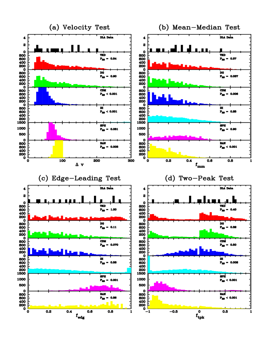
Figure 10: Plot of the $\Delta v$, ${f_{\rm edg}}$, ${f_{\rm mm}}$, and ${f_{\rm 2pk}}$ distributions for the data and the six test models. The $P_{KS}$ values represent the probability the test distribution and the data could have been drawn from the same parent population. Note that every model except the TRD Model is inconsistent with the data for one or more statistical tests.

Figures 10a$-$d show comparison plots of the 4 test statistics for each of the 6 kinematic models. After an exhaustive search of the parameter space ${\rm\underline{permitted}}$ by each model, we chose those parameters yielding the closest agreement to the data. Table 3 gives the parameters used in the simulations, while the $P_{KS}$ values are listed in Table 4. The Figure demonstrates that apart from “cold” disks with high rotation speeds, the remaining models are ruled out at high levels of confidence by at least 1 statistical test. Therefore, of all the tested models, only “cold” disks with rapid rotation are consistent with the damped Ly$\alpha$ kinematics. In the following subsections, we will briefly discuss why the other models fail specific tests and why improved results are unlikely.

Table 3: MODEL PARAMETERS

MODEL	$N_{\perp}(0)$	$v_{rot}$ or $v_{0}$	$\sigma_{cc}$	$n_{c}$	$h$
	($\,\rm cm^{-2}$)	(km s-1 )	(km s-1 )	$(2{\rm\;\times\;10^{20}})$	$(r_{0})$
TRDa	21.2	250	10	5	0.4
DGb	21.2	50	5-55	5	0.3
CDMc	21.2	30-200	10	5	0.3
IHd	–	40	190	10	–
SPHe	19.4	20	10	5	–
RANf	–	100	–	15	–

^a Cold, Rapidly Rotating Disk Model

^b Dwarf Galaxy Model

^c Cold Dark Matter Model

^d Isothermal Halo Model

^e Spherical Accretion Model

^f Random Motions Model

Table 4: $P_{KS}$ VALUES

MODEL	VEL	MM	EDG	TRD
TRD	0.84	0.37	0.99	0.40
DG	0.90	0.034	0.11	0.31
CDM	$2.0{\rm\;\times\;10^{-4}}$	0.0062	0.070	0.49
IH	$4.5{\rm\;\times\;10^{-16}}$	0.25	0.58	0.0016
SPH	0.030	0.90	0.0015	$1.0{\rm\;\times\;10^{-8}}$
RAN	0.0034	4.5 ${\rm\;\times\;10^{-4}}$	0.86	$4.0{\rm\;\times\;10^{-6}}$

6.1 Models with Rotating Disks

Rotating disks are essential elements in models with “cold” disks of giant spirals, “hot” disks of dwarf galaxies, and the progenitors of spiral galaxies in CDM cosmologies. The models considered in this subsection have the properties discussed in $\S$ 3, and differ only in the choice of the parameters $v_{rot}$, $\sigma_{cc}$, $h/R_{d}$, $n_{c}$ and $N_{\perp}(0)$.

6.1.1 “Cold” Disks of Giant Spirals

In this model, velocity profiles are generated by line-of-sight impacts through a set of intrinsically identical exponential disks that are “cold” and rapidly rotating. Therefore, all the input parameters are the same for each of the 8,500 impacts comprising a given run. In order for the H I disks to be “cold” we let $\sigma_{cc}$ = 10 km s^-1 which equals the velocity dispersion measured across the H I disks of spiral galaxies [van der Kruit & Shostak 1984]. Note the results are insensitive to the value of $\sigma_{cc}$ provided $\sigma_{cc}<25$ km s^-1 ; i.e., the disks remain “cold”. For larger values of $\sigma_{cc}$, the model fails the Two-Peak Test and also cannot reproduce the low $\Delta v$ tail of the Velocity Interval Test distribution. For each run we set $v_{rot}$ = 250 km s^-1 and $h/R_{d}$ = 0.4. This rotation speed is a representative value for current giant spirals [Rubin et al. 1985]. The scale-height is chosen to reproduce the observed distribution of $\Delta v$.

As this model assumes identical properties for all intercepting galaxies, it is somewhat naive. A more realistic model would include a distribution of rotation speeds, thicknesses and central column densities. However, it is valuable for testing the null hypothesis that giant spirals explain the kinematic state of the damped Ly$\alpha$ systems. The figures show that the null hypothesis cannot be ruled out for this model, because it produces acceptable values of $P_{KS}$ for each of the 4 statistical tests.

6.1.2 “Hot” Disks of Dwarf Galaxies

In this model we assume the velocity profiles are generated by the disks of dwarf galaxies in which $\sigma_{cc}$ is assumed to vary from object to object. York et al. (1986) first suggested dwarf galaxies were responsible for QSO absorption systems exhibiting metal lines. More recently, Pettini et al. (1994) and Lu et al. (1996b) advocated dwarfs as the site of damped Ly$\alpha$ absorption. These authors were struck by the similarity between the low metallicities and element abundance patterns in dwarfs and damped Ly$\alpha$ systems.

The velocity profiles are generated by the same algorithms used to model the “cold” disks discussed in the previous subsection. That is, except for $\sigma_{cc}$, all the input parameters are fixed for the profiles computed in each of 8,500 galaxy impacts. However, for these disks we assume $v_{rot}$ = 50 km s^-1 which is a good representation for the rotation speeds of dwarf irregulars [Freeman 1993]. We draw $\sigma_{cc}$ from a distribution spanning velocities between 5 and 55 km s^-1 in such a way that the resultant $\Delta v$ matches the data. The range in $\sigma_{cc}$ simulates the episodic turbulence originating from the high frequency of supernova remnants that might occur at large redshifts. The idea is to let random motions in gas accelerated by supernova activity produce the observed $\Delta v$. This was suggested earlier as the explanation behind the large $\Delta v$ detected in metal line absorbers as well as damped Ly$\alpha$ systems [York et al. 1986, Pettini et al. 1994]. Of course, if we were to require $\sigma_{cc}\ll 55$ km s^-1 always (as observed in local gas-rich dwarfs), the model fails a priori as it cannot reproduce the velocity widths, $\Delta v>100$ km s^-1 . Finally, to further enhance $\Delta v$ we set $h/R_{d}$ = 0.3.

Because the kinematics of the “hot” dwarf galaxy model are influenced by velocities randomly drawn from a Gaussian distribution, the simulated profiles tend to peak symmetrically about $v=0$ km s^-1 . As a result the model profiles yield discrepant ${f_{\rm mm}}$ statistics; $P_{KS}({f_{\rm mm}})=0.037$. Furthermore, the model is only marginally consistent with the Edge-Leading Test as $P_{KS}(f_{edg})$ equals 0.11. Note that the model survives the Two-Peak Test, because a large fraction of the profiles are produced with a single peak, which as noted above, biases the distribution to positive values in the $f_{2pk}$ distribution.

We wish to point out that these results are significantly dependent on both the assumed cloud number $n_{c}$ at threshold ${N({\rm HI})}$ (taken to equal 5) and $\sigma_{cc}$. Specifically, increasing $n_{c}$ while holding $\sigma_{cc}$ constant will increase the range of $\Delta v$ values due to the greater sampling of the random Gaussian distribution. Similarly, increasing $\sigma_{cc}$ while holding $n_{c}$ constant has the same effect. At the same time, increasing $n_{c}$ reduces the level of asymmetry as the random motions begin to dominate the rotation kinematics. We find that the threshold $n_{c}=5$ gives the best agreement to all four statistical tests, and that models with threshold $n_{c}>10$ are ruled out at higher confidence levels, because both $P_{KS}({f_{\rm mm}})$ and $P_{KS}({f_{\rm edg}})$ would be less than 0.01.

6.1.3 Disk Progenitors in CDM Cosmology

Kauffmann (1996) recently combined Press-Schecter theory with the Cold Dark Matter cosmology (CDM) to compute the hierarchical merging of protogalactic disks embedded in dark-matter halos. Semi-analytic techniques were used to calculate the formation of

H I disks as gas cools and accretes in the merging halos. With the damped Ly$\alpha$ systems in mind, Kauffmann (1996) computed $P(v_{rot})$, the interception probability presented by the cross-sectional area of the disks, as a function of $v_{rot}$ for various redshifts. The radial distribution of H I column densities, $N_{\perp}(R)$ was also computed for different values of $v_{rot}$.

We calculated velocity profiles for this model as follows. For each of the 8,500 impacts comprising a given run we drew $v_{rot}$ randomly from the $P(v_{rot})$ corresponding to the redshift $z$ = 2.5, in good agreement with the average redshift, $z$ = 2.48, of the profiles in our statistical sample. We then fitted exponential profiles to the plots of $N_{\perp}(R)$ by assuming $N_{\perp}(0)=10^{21.2}\,\rm cm^{-2}$. Kauffmann (1996) implicitly assumed the disks to be thin, $h$ $<<$ $R_{d}$, and “cold”, $\sigma_{cc}$ $<<$ $v_{rot}$. Because $v_{rot}$ is less than 100 km s^-1 in 70$\%$ of the model disks, the predicted distribution of $\Delta v$ will not match the observed distribution which extends out to 200 km s^-1 . Therefore, we assumed $h$ = 0.3$R_{d}$ to maximize $\Delta v$ without significantly changing the disk-like character of the model. Otherwise, we followed the same procedures used to compute velocity profiles for the other disk models.

The results shown in Figure 10 indicate this model is highly unlikely to represent the data. Owing to the predominance of slowly rotating disks, the Velocity-Interval and Mean-Median Tests result in $P_{KS}({\Delta v})$ $<$ 0.001 and $P_{KS}(f_{mm})$ = 0.002 which are unacceptable. Had we increased $N_{\perp}(0)$ to $10^{22.2}\,\rm cm^{-2}$, which is closer to the value Kauffmann derived, the $\Delta v$ distribution would peak at even lower velocities, owing to the “column-density kinematic” effect, and could be ruled out at even higher confidence levels. Consequently we conclude this CDM model is ruled out at high levels of confidence. Even if we were to ignore the two highest $\Delta v$ values, this CDM model is still ruled out at $>99\%$ c.l. The implications of this important result for theories of galaxy formation are discussed in $\S$ 9.

6.2 Models Without Rotating Disks

We now turn to models without rotating disks.

6.2.1 Isothermal Halos

In order to mimic the kinematics of the Galaxy halo, we let the halo gas rotate with $v_{rot}(r)=50$ km s^-1 , and assume $\sigma_{cc}=190$ km s^-1 (see Majewski 1993). As in $\S$ 3.2 we set $\sigma_{int}$ = 4.3 km s^-1 . For the isothermal sphere we choose the central mass density, $\rho_{0}$, in such a way that the mass $M$($r$=20 kpc) = 2$\times$10¹¹$M_{\odot}$, which is the mass inferred from a constant disk rotation speed $v_{rot}$ = 220 km s^-1 out to $\approx 20\;\rm{kpc}$. The length scale of the density distribution, i.e., the King radius, is then determined by the relation, $r_{0}$ = $\sqrt{9{\sigma_{cc}^{2}}/(4{\pi}G{\rho_{0}})}$ and equals 18 kpc. However, because the kinematics are dominated by the random motions of the clouds, the results are essentially independent of $\rho_{0},r_{0}$, and the assumed density profile.

To generate simulated spectra we follow the prescription of $\S$ 3.2, except that the $(X,Y)$ coordinates are drawn from a projected circle rather than a projected ellipse. The circle has a radius $r$ = $R_{f}$, where $R_{f}$ has the same meaning as in $\S$ 3.2. We also assume the angular momentum of the gas defines a preferred plane whose rotation axis is a random variable.

Figure 10a shows that the value of $\sigma_{cc}$ is sufficiently large to throw most of the distribution of $\Delta v$ off scale, peaking at $\Delta v\approx 600$ km s^-1 . As a result the model fails the $\Delta v$ test at a very high level of confidence. Furthermore, $P_{KS}({f_{\rm 2pk}})<0.002$ owing to the large fraction of ${f_{\rm 2pk}}<0$ resulting from the random locations of the absorption peaks. We tried to decrease $\Delta v$ by reducing $n_{c}$ from 10 to 5, but this increased the fraction of profiles with ${f_{\rm 2pk}}<0$, and consequently produced an even lower $P_{KS}({f_{\rm 2pk}})$ value. Because $\sigma_{cc}$ $>>$ $v_{rot}$, this model, like the dwarf galaxy model, generates profiles exhibiting a high degree of symmetry in the limit $n_{c}\gg 1$. However, in this simulation $\sigma_{cc}$ is so large that for $n_{c}=10$, it is rare for two clouds to overlap in velocity space. Therefore, the strongest absorption peak occurs randomly due to the noise in the spectrum. Because this leads to an ${f_{\rm edg}}$ distribution similar to that of the Random Motions Model, $P_{KS}({f_{\rm edg}})=0.58$. By the same reasoning, the asymmetry is accentuated such that $P_{KS}({f_{\rm mm}})=0.25$. However, we find that for $n_{c}>15$, all Isothermal Halo Models are ruled out by the Mean-Median and Edge-Leading Tests.

6.2.2 Spherical Accretion

We modeled the accretion flow with a central bulge having mass $M\approx 10^{10}M_{\odot}$ and gas with sound speed $v_{0}\approx a_{\infty}$ = 20 km s^-1 implying $r_{s}\approx$ 110 kpc. The sound speed is physically reasonable and is chosen to roughly reproduce the observed $\Delta v$ distribution. However, it corresponds to thermal temperatures high enough that the gas will be collisionally ionized. Thus the gas creating damped Ly$\alpha$ absorption must be discrete neutral clouds embedded in a smooth, ionized medium.

By contrast with the other models in this section, the kinematics of the spherical infall model are dominated by systematic motions, i.e. radial infall, rather than random motions. However, the profiles are still symmetric with the peaks tending to lie at both edges of the velocity interval. As a result, the Two-Peak Test distribution is dominated by negative $f_{2pk}$ for all values of $n_{c}$, $v_{0}$ and $n_{0}$, in contradiction to the empirical $f_{2pk}$ distribution which is why $P_{KS}({f_{\rm 2pk}})<0.001$. Furthermore, while the model predicts a peak in the $f_{edg}$ distribution near $f_{edg}$ $\approx$ 0.75, the empirical distribution is more uniform between 0 and 1.0. Thus the profiles predicted by the spherical infall model are actually too “edge-leading”, and as a result $P_{KS}({f_{\rm edg}})=0.001$. Note, in order to reproduce the observed $\Delta v$ distribution we developed ad hoc distributions of $v_{0}$. The combined weight of the tests rule out this model at very high confidence levels.

6.2.3 Random Motion Models

The Random Motion Model assumes a uniform deviate yielding less symmetric, more edge-leading profiles than those models with a Gaussian deviate. Owing to the uniform deviate, the strongest peak is distributed uniformly within the velocity interval. As a result the model yields acceptable values of $P_{KS}(f_{edg})$ for a wide range of cloud numbers. However, the profiles are still too symmetric for consistency with the Mean-Median Test for all but the smallest values of $n_{c}$. And the model fails the Two-Peak Test and, the Velocity Interval Test for all values of $n_{c}$. Therefore, this model is highly unlikely to represent the data. As in our treatment of the dwarf galaxies, we also considered a model (not plotted in Figure 10) in which $\Delta v$ is drawn uniformly from a distribution designed to give an acceptable distribution of $\Delta v$. Although this model yields $P_{KS}(\Delta v)\approx 1$, it is ruled out at high confidence levels by both the Mean$-$Median and Two$-$Peak Tests.

7 PROPERTIES OF ROTATING DISKS RESPONSIBLE FOR THE DAMPED Ly$\alpha$ SYSTEMS

Apart from rapidly rotating “cold” disks and slowly rotating “hot” disks, every model we tested is ruled out at higher than 99.9 $\%$ confidence by one or more of the tests. Because the “hot disks”, i.e., the turbulent dwarf galaxies, are ruled out at $97\%$ confidence, the only considered models compatible with the kinematic data are those with rapidly rotating “cold” disks. In order to place more rigorous bounds on parameters such as rotation speed and disk thickness, we investigate the parameter space of these models. In particular we perform Monte Carlo runs for a wide range of the parameters $v_{rot}$, $h/R_{d}$, and $N_{\perp}(0)$. Although we compute all four test statistics for each run, only the $\Delta v$ distributions are particularly sensitive to variations of $v_{rot}$, $h/R_{d}$, and $N_{\perp}(0)$. Therefore, we confine the discussion to the $\Delta v$ distributions, and to models with identical disks.

The results are shown in Figure 11 (left side) as iso-probability contours in the $h/R_{d}$, $v_{rot}$ plane for $N_{\perp}(0)$ = (a) $10^{20.8}\,\rm cm^{-2}$, (b) $10^{21.2}\,\rm cm^{-2}$, and (c) $10^{21.6}\,\rm cm^{-2}$. The contours correspond to selected values of $P_{KS}(\Delta v)$, the KS probability discussed in $\S~{}\ref{rstssec}$. Because the KS test is better suited for ruling out rather than establishing null hypotheses, these contours indicate the range of $v_{rot}$ and $h/R_{d}$ excluded by the data; in particular, thin disks with slow rotation are unlikely.

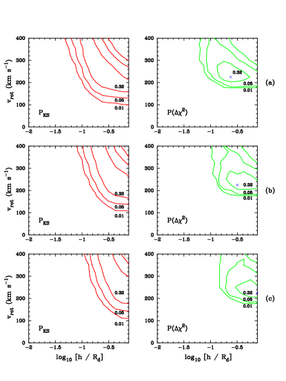
Figure 11: Left Panels show isoprobability contours from the $P_{KS}({\Delta v})$ tests in the $v_{rot}$, $h/R_{d}$ plane for the cold rotating disk model with $N_{\perp}(0)=$ (a) $10^{20.8}\,\rm cm^{-2}$, (b) $10^{21.2}\,\rm cm^{-2}$, and (c) $10^{21.6}\,\rm cm^{-2}$. Contour levels are drawn at $P_{KS}({\Delta v})$ = 0.01, 0.05, and 0.32. Right panels show isoprobability contours derived from the Likelihood Ratio Test with the same contour levels. Note that disks with rotation speeds $v_{rot}<180$ km s^-1 or thickness $\log[h/R_{d}]<-1.0$ are extremely unlikely.

To find the most likely range of parameters, we turn to the Likelihood Ratio Test. Define the likelihood,

$$L\equiv\prod\limits_{i=1}^{n_{d}}p(\Delta v_{i})\;\;\;,$$ (15)

where $p(\Delta v_{i})$ is the probability a model yields the velocity interval, $\Delta v_{i}$, assigned to the $i^{th}$ member of a sample comprising $n_{d}$ damped Ly$\alpha$ systems. We compute $L_{max}$, the maximum value of $L$ with respect to the parameters, i.e., we maximize the function $L=L(v_{rot},h/R_{d},N_{\perp}(0))$ in the $v_{rot}$, $h/R_{d}$ plane or the $v_{rot}$, $N_{\perp}(0)$ plane. For the $v_{rot}$, $h/R_{d}$ plane the maximal points are indicated by the $\times$’s on the right side of Figure 11. We then compute the probability $-2\ln(L/L_{max})$ which is asymptotically distributed as $\Delta\chi^{2}$ for 2 degrees of freedom in either plane, where $\Delta\chi^{2}$ = $\chi^{2}$ $-$ $\chi^{2}_{min},$ and $\chi^{2}_{min}$ is $\chi^{2}$ at the maximal point. The contour levels on the right side of Figure 11 are the confidence levels corresponding to $\Delta\chi^{2}\geq-2\ln(L/L_{max})$ for $N_{\perp}(0)$ = (a) $10^{20.8}\,\rm cm^{-2}$, (b) $10^{21.2}\,\rm cm^{-2}$, and (c) $10^{21.6}\,\rm cm^{-2}$. When $N_{\perp}(0)=10^{21.6}\,\rm cm^{-2}$, $L_{max}$ lies on the edge of the parameter space we investigated and as a result determination of the “true” maximum is uncertain. We do not consider configurations with $\log[h/R_{d}]>-0.25$ as they do not qualify as disks. Therefore, it is possible that the contours with this $N_{\perp}(0)$ will encompass an even smaller area in this parameter space.

The Likelihood Ratio Test results in several significant trends. First, a lower limit of $v_{rot}>180$ km s^-1 is established at the $99\%$ confidence level, independent of $N_{\perp}(0)$ and $h/R_{d}$. Upper limits on $v_{rot}$ are less restrictive, especially for smaller values of $h/R_{d}$ and larger $N_{\perp}(0)$. In fact there is a portion of parameter space allowing $v_{rot}>375$ km s^-1 at the 95$\%$ confidence level for all 3 values of $N_{\perp}(0)$. But in every case the optimal rotation speed is given by $v_{rot}\approx$ 225 km s^-1 . Also note that the $95\%$ and 99$\%$ contours have larger areas when $N_{\perp}(0)=10^{20.8}\,\rm cm^{-2}$, a trend caused by the “column-density kinematic” effect discussed in $\S~{}\ref{MCmthds}$. This is further illustrated in Figure 12 which is an iso-probability contour plot of $v_{rot}$ vs. $N_{\perp}(0)$ for $h/R_{d}$ = 0.3. The gradual rise of $v_{rot}$ with increasing $N_{\perp}(0)$ indicates larger rotation speeds are required to compensate for the narrower profiles produced when $N_{\perp}(0)$ is large. Second, the optimal $h/R_{d}$ value is at 0.32. While we find a lower limit of $h/R_{d}$ $>$ 0.1 at the 99$\%$ confidence level, the test places no upper limit on $h/R_{d}$. This is because the gradient of $v_{rot}$ along the line of sight increases with $h/R_{d}$ until it remains nearly constant at $h/R_{d}$ $\geq$ 0.4.

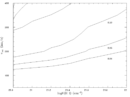
Figure 12: Isoprobability contours of $P_{KS}({\Delta v})$ values in the $v_{rot}$, ${N({\rm HI})}$ plane with $h/R_{d}=0.3$. The contour levels are drawn at $P_{KS}=$ 0.01, 0.05, and 0.32. The figure demonstrates that higher rotation speeds are required as $N_{\perp}(0)$ increases.

Finally, we consider the robustness of our results, in particular the optimal rotation speed, $v_{rot}=225$ km s^-1 , found from maximum likelihood techniques. First, we believe the rotation speed must be large simply because there is no evidence that the $\Delta v$ with the largest values are spurious outliers. Rather, the distribution out to large $\Delta v$ contains a tail which is real; for example, 6 of the 17 profiles have $\Delta v>120$ km s^-1 . However, our single population model with $v_{rot}$ the same for all disks is naive in that it cannot explain the detection of a single system with $\Delta v>225$ km s^-1 . In a more realistic multi-population model, $v_{rot}$ would be distributed out to 350 km s^-1 in order to explain the largest rotation speeds measured for current Sa spirals [Rubin et al. 1985]. Such a model could then explain $\Delta v\leq 350$ km s^-1 . Higher values would then have to be interpreted in terms of multiple disks or some other mechanism.

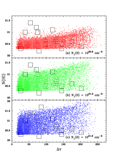
Figure 13: Plot of ${N({\rm HI})}$ vs $\Delta v$. Clear squares represent the data. Dots represent simulation results for three runs with $h/R_{d}=0.3$, and $N_{\perp}(0)=$ (a) $10^{20.8}\,\rm cm^{-2}$, (b) $10^{21.2}\,\rm cm^{-2}$, and (c) $10^{21.6}\,\rm cm^{-2}$.

While the statistical tests show the general features of the “cold” disk models are consistent with observation, the assumption of identical $N_{\perp}(0)$ may be incorrect. Figure 13 is a plot of observed $N$(H I) vs $\Delta v$ for $N_{\perp}(0)$ = (a) $10^{20.8}\,\rm cm^{-2}$, (b) $10^{21.2}\,\rm cm^{-2}$, and (c) $10^{21.6}\,\rm cm^{-2}$. Although the data exhibit a possible anti-correlation between $N$(H I) and $\Delta v$, all three models predict a positive correlation between these quantities. The correlation arises because low $\Delta v$ are generally produced at large impact parameters where $N$(H I) is small and large $\Delta v$ are produced at small impact parameters where $N$(H I) is large. Better agreement with the data could be achieved by dropping the unrealistic assumption of identical $N_{\perp}(0)$. Thus some contribution from disks with $N_{\perp}(0)$ = 10^21.6 cm^-2 would help to explain data points with $N$(H I) $>$ 10^21.2 cm^-2, while disks with $N_{\perp}(0)$ = 10^20.8 cm^-2 help to explain the distribution of data points at $N$(H I) $<$ 10^20.8 cm^-2. But even this scheme produces too many disks with $\Delta v$ $<$ 60 km s^-1 and $N$(H I) $<$ 10^20.8 cm^-2. These might be eliminated by invoking photoionization of the outer disks where the gas density is low and ionization parameter high. We are currently experimenting with these and other schemes in order to obtain a better match with the data.

8 AN INDEPENDENT TEST FOR RAPIDLY ROTATING DISKS

Recently Ly$\alpha$ emission, at $z$ = 3.15, was detected from an object displaced by 2.3 arcsec from a sightline intersecting a damped Ly$\alpha$ system with a similar redshift (Djorgovski et al. 1996). This suggests a test of the rotating disk hypothesis. Let the emission come from the center of the gaseous disk causing absorption. The geometry of such a configuration is illustrated in Figure 14. The circle represents a disk rotating with $v_{rot}$ in the counterclockwise direction as indicated by the velocity vectors. Two possible sightline geometries are indicated by the vertical dashed lines that run from the observer at the bottom to the QSO at the top of the figure. The kinematic major axis of the disk is the dash-dot-dash line. The dots at positions 1$-$4 show four locations where the sightlines encounter the disk midplane. The metal-line velocity profiles in the figure were computed according to the algorithms of $\S$ 3.2 which describes why “edge-leading” profiles arising from midplane encounters far from the major axis, as in positions 1 and 4, exhibit asymmetries that mirror “edge-leading” profiles arising from midplane encounters near the major axis, as in positions 2 and 3. The figure shows the emission redshift, $v$ = 0, lies at or beyond the boundaries of the absorption profile in every case. Furthermore, the component with peak optical depth should be at the profile boundary nearest to $v$ = 0, when the point of midplane encounter is far from the major axis or farthest from $v$ = 0, when the midplane encounter is nearer to the major axis.

As a result, the disk model predicts a systematic relation between the kinematics of emission and absorption lines. By contrast the peak component would be randomly distributed with respect to $v$ = 0, were damped Ly$\alpha$ absorption to arise in undetected satellite galaxies bound to massive primary galaxies detected in emission. Suppose the speed of the satellite with respect to the primary is given by $v_{sat}$, and the internal kinematics of the satellite generates a profile with velocity interval, $\Delta v$. The probability that the emission redshift of the primary is within $\Delta v$ is then given by

$$P_{profile}=(1/2)\left\{\begin{array}[]{ll}{\Delta v}/v_{sat},&{\Delta v}<v_{sat}\\ 1,&{\Delta v}\geq v_{sat}.\end{array}\right.$$ (16)

Therefore, when $\Delta v$ $<<$ $v_{sat}$, the satellite-primary configurations are unlikely to produce emission redshifts within the absorption profile, and are thus indistinguishable from absorption by a single large disk. But when $\Delta v$ $\approx$ $v_{sat}$, the emission redshifts are likely to lie within $\Delta v$. Because $v_{sat}$ $>$ 100 km s^-1 [Zaritsky & White 1995], a significant fraction of absorption profiles with $\Delta v$ $>$ 100 km s^-1 should contain the emission redshift, if the satellite/primary galaxy hypothesis is correct. Clearly, the combination of emission and absorption kinematics provides powerful and independent tests of the rotating disk model.

Such a test was initiated by Lu et al. (1996b). They used HIRES to obtain low-ion profiles for the $z_{abs}$ = 3.15 damped Ly$\alpha$ absorber toward Q2233$+$131, the same system Djorgovski et al. (1996) found to be associated with an emitting galaxy at the absorption redshift. Comparison between emission and absorption profiles shows the centroid of the emission line is located outside the absorption profile characterized by $\Delta v$ = 200 km s^-1 . This is consistent with the kinematics of a large, rotating disk centered on the Ly$\alpha$ emitter. Because the peak component is at the profile boundary farthest from $v$ = 0, the point of midplane encounter should be near the major axis. Lu etal (1996b) used their measurement of $\Delta v$ to set a lower limit of 200 km s^-1 on $v_{rot}$ which was combined with the impact parameter, $b$ = 30$h_{50}^{-1}$ kpc, to deduce a total mass for the galaxy of $M_{gal}$ $>$ $3\times 10^{11}h_{50}^{-1}\rm M_{\odot}$ (note this mass is somewhat higher than the [Lu et al.  1996b] estimate, since we assume $\Omega_{0}$ = 0.1 rather than $\Omega_{0}$ = 1.0). On the other hand the combination of large values for $b$ and $\Delta v$ raises potential problems for the big disk interpretation, because the column-density velocity effect ($\S$ 3.2) indicates small $\Delta v$ when $b/R_{d}$ is large. Perhaps $b/R_{d}$ is small in this case because $R_{d}$ exceeds 10 kpc, as expected from the high incidence of damped Ly$\alpha$ systems along the line of sight. Moreover a large inclination angle, $i$ $>$ 80⁰, would also increase $\Delta v$.

Figure 14: Same as Figure 3 except here we show 2 sightlines (dashed vertical lines). In the profiles, the emission redshift, $v=0$, lies at or beyond the boundaries of the absorption profile in every case and the strongest feature lies at one of the edges.

9 CONCLUDING REMARKS

Our principal result is the CDM scenario for the formation of galactic disks predicts rotation speeds at $z$ $\approx$ 2.5 that are ruled out at high confidence levels by the neutral-gas kinematics in damped Ly$\alpha$ systems. Specifically, the semi-analytic model of Kauffmann (1996) predicts most precursors of current massive spirals to be disks embedded in dark-matter halos with masses less than $\approx$ 10¹⁰$M_{\odot}$ and rotation speeds less than 100 km s^-1 . By contrast, the likelihood ratio test in $\S$ 8 requires minimum rotation speeds, $v_{rot}$ $>$ 180 km s^-1 , at the 99 $\%$ confidence level. The most likely value, $v_{rot}=225\rm\;km\;s^{-1}.$ While estimates of the masses responsible for rotation are not generally available, the $3\times 10^{11}h_{50}^{-1}\rm M_{\odot}$ lower limit set for the galaxy at $z$ = 3.15 is an important constraint, because galaxies with such large masses rarely contain disks with significant gaseous cross sections at large redshifts in hierarchical scenarios [White & Frenk 1991, Kauffmann 1996]. Rather our impression is that disks embedded in low-mass halos causing low rotation speeds dominate the damped Ly$\alpha$ interception probabilities in most hierarchical models. We will check this impression by using our Monte Carlo techniques to test the predictions of other independent CDM models (see the numerical models of [Katz et al. 1996]) and Hot $+$ CDM models [Klypin et al. 1995]. Furthermore, we will test the recent suggestion that damped Ly$\alpha$ absorption arises in multiple low-mass galaxies rather than in a single object [Rauch et al. 1996, Gardner et al. 1996]. However, until such schemes are shown to be consistent with the kinematic data, we shall adopt the idea of large, rapidly rotating disks that formed prior to $z$ $\sim$ 3 as a working hypothesis for the damped Ly$\alpha$ systems. We note the early formation of large disks in massive galaxies is a signature of the isocurvature models [Peebles 1993, Peebles 1996], and possibly hierarchical models where $\Omega_{0}\ll 1$ and $\Lambda=0$.

Let us take a closer look at the rapidly rotating disk model. First, we assumed the rotation curve was flat for all radii. This is true in current spirals, owing to a coincidence at small radii of (i) the sum of the radial gravitational forces due to stellar disk and bulge, and (ii) the radial gravitational force due to the dark-matter halo [Binney and Tremaine 1987]. However, in damped Ly$\alpha$ systems the force due to the disk is small compared to the halo or bulge (the evidence for bulges in damped Ly$\alpha$ systems stems from the recent detection of damped Ly$\alpha$ absorption, at the emission redshift, in the spectrum of a Lyman-break bulge at $z$ = 2.7 [Steidel 1996]), because the surface densities of the gaseous damped Ly$\alpha$ disks are low compared to the surface densities of stellar disks in current spirals. For example the central surface densities of disk-population stars in spirals like the Galaxy are typically 500 to 1000 $M_{\odot}$pc^-2, whereas the central surface densities of gas in damped Ly$\alpha$ systems are at least 10 times smaller (see [Wolfe et al. 1995]). As a result rotation curves in damped systems should behave as follows. In the absence of a bulge, the rotation speed due to a spherical isothermal halo rises out to the core radius and remains flat at larger radii. The presence of a bulge in the damped Ly$\alpha$ system results in a steeper rise from $R$ = 0 because of the smaller core radius of the bulge. At larger radii the rotation speed will drop and then rise again at radii sufficiently large for the halo to dominate. Sightlines penetrating these types of disks may produce $\Delta v$ smaller than predicted by our model. We are currently constructing self-consistent models including bulge, disk, and halo components. Second, we assumed $v_{rot}$ was independent of $Z$. In a self-consistent model the azimuthal velocity, $v_{\phi}(R,Z)$, would decrease with increasing $Z$ because the $R^{th}$ component of the radial force decreases with $Z$ for spherically symmetric mass distributions. We carried out some preliminary tests of this effect by imposing a negative $Z$ gradient on $v_{rot}$. Specifically, we let $v_{rot}$ vary linearly from 225 km s^-1 at $Z$ = 0 to 150 km s^-1 at 1 kpc and found the gradient had only minor effects on the test statistics. Third, we are investigating the limits ionizing radiation places on the sizes of the gaseous disks and its effect on the test statistics.

Having explored the gas we turn to the stars by speculating about possible stellar byproducts of the damped Ly$\alpha$ disks. The kinematic evidence points to disks that: (1) are rapidly rotating, $v_{rot}$ $\approx$ 225 km s^-1 ; (2) are “cold”, $\sigma_{cc}$ $<<$ $v_{rot}$; and (iii) may have large scale heights, since $h$ $>$ 0.1$R_{rad}$. By contrast the abundance measurements bring to mind “hot” configurations in which $\sigma_{cc}$ $>>$ $v_{rot}$. This is because the low metallicity, [Zn/H] = $-$1.2 [Pettini et al. 1994] or [Fe/H] = $-$ 1.5 [Lu et al.  1996b], and the relative abundance patterns, suggesting gas enrichment only by type II supernovae [Lu et al.  1996b], are signatures of halo population II stars. Therefore the kinematic and chemical evidence are in conflict.

The conflict might be resolved if star formation in damped Ly$\alpha$ disks results in a thick, metal-poor disk not unlike the thick stellar disk of the Galaxy [Gilmore, Wyse & Kuijken 1989]. The latter is characterized by scale height $h$ $\approx$ 1.5 kpc. The scale height is compatible with $h$ $>$ 0.1$R_{d}$ inferred for the damped systems because $R_{d}$ for current spirals ranges between 3 and 6 kpc [Kent 1986], and $R_{d}$ for high-$z$ damped systems must be more than twice these values to explain their incidence along the line of sight [Lanzetta 1993]. However, it is not obvious that the assumed velocity dispersion, $\sigma_{cc}$ = 10 km s^-1 , can maintain matter, gas or stars, at scale heights as large as 1.5 kpc. At the solar neighborhood, where the surface density $\Sigma$ = 70 $M_{\odot}$pc^-2, stars with $\sigma_{cc}$ $\approx$ 25 km s^-1 have a scale height $h$ = 0.4 kpc [Mihalas and Binney 1981]. Because the disk models fail the Velocity Interval and Two Peak tests when $\sigma_{cc}$ $>$ 25 km s^-1 , large physical scale heights could be a serious problem for the disk model. However, the average surface density for damped Ly$\alpha$ systems is only $\approx$ 10$M_{\odot}$pc^-2, and since $\sigma_{cc}$ $\propto$ $(h{\Sigma})^{1/2}$ for self-gravitating disks, $h$ $\sim$ 1.5 kpc is in principal compatible with $\sigma_{cc}$ $<$ 20 km s^-1 . On the other hand, the damped Ly$\alpha$ disks may be self-gravitating only at $R$ $<$ $R_{d}$. This is because the vertical structure of the disk is controlled by dark matter in the halo rather than self gravity at $R$ $>$ $R_{d}$ for exponential disks with central surface densities low compared to that of the Galaxy (Gunn 1982). In the dark-matter limit $h$ $\approx$ $\sigma_{cc}$$R$/$v_{rot}$ and $\sigma_{cc}$ $\approx$ 10 km s^-1 . As a result thick disks with low velocity dispersions may be physically plausible at any radius. While we have not run simulations in which $h$ $\propto$ $R$, we see no reason why “flaring” disks would dilute the asymmetries required to explain the line profiles.

Other parameters characterizing the thick stellar disk are the mass fraction, rotation speed, and metallicity. The mass fraction, $M_{thick\ disk}/M_{thin\ disk}$ $\approx$ 0.1. This could be explained by a 10 $\%$ decrease of $\Omega_{g}(z)$ between $z$ = 3 and 1.5, which is consistent with the observed variation of $\Omega_{g}(z)$ [Storrie-Lombardi and Wolfe 1997]. The rotation speed is given by $v_{rot}$ $\approx$ 150 km s^-1 . Although this is lower than the optimal rotation speed, $v_{rot}$ = 225 km s^-1 , a vertical velocity gradient going from $v_{rot}$ = 225 km s^-1 at midplane to 150 km s^-1 at $Z$ $\approx$ $h$ would explain the kinematics and results in simulated test-statistics compatible with the data, as discussed above. The most difficult problem has to do with metallicity, because the average [Fe/H] for the damped systems is between a factor of 4 and 10 below the mean metallicity of the thick disk, $\langle$[Fe/H]$\rangle$ = $-$0.6 [Gilmore, Wyse & Kuijken 1989]. However, the thick disk abundance data refer only to stars near the solar circle, whereas the relevant metallicity is an average over the entire thick disk, which is unknown. As a result [Fe/H] averaged over thick stellar disks would range between $-$1.2 and $-$1.6 in this scenario.

Finally we cannot rule out the possibility that a significant fraction of the neutral gas experiences negligible star formation between $z$ = 3 and 1.5. In that case the descendents of damped Ly$\alpha$ systems would be extended metal-poor configurations of gas surrounding the visible parts of galaxies. The detection of low metallicity damped Ly$\alpha$ systems at low redshifts, $z$ $<$ 1, provides evidence for such gas [Meyer et al. 1995]. In this case the agreement between the comoving density of neutral gas at $z$ $\approx$ 3 and the density of visible matter in current galaxies would refer to the inner disks where star formation occurs, presumably at $z$ $<$ 1.5.

We are deeply indebted to the group headed by W. L. W. Sargent for generously providing us with their HIRES spectra. We are especially grateful to Limin Lu for extensive discussions and comments. The authors would also like to thank Tom Barlow for his excellent HIRES data reduction software. We also thank Kim Griest, Ken Lanzetta, Jim Peebles, Joe Silk, David Tytler, and Amos Yahil for stimulating discussions. AMW and JXP were partially supported by NASA grant NAGW-2119 and NSF grant AST 86-9420443.

References

- [Arons 1972] Arons, J. 1972, ApJ, 172, 553
- [Barlow 1997] Barlow, T. 1997, in preparation.
- [Binney and Tremaine 1987] Binney, J. and Tremaine, S. 1987, Galactic Dynamics (Princeton: Princeton University Press), p. 229
- [Briggs et al.1985] Briggs, F.H., Turnshek, D.A., Schaeffer, J., and Wolfe, A.M. 1985, ApJ, 293, 387
- [Briggs et al. 1989] Briggs, F. H., Wolfe, A. M., Liszt, H. S., Davis, M. M., and Turner, K. L. 1989, ApJ, 341, 650
- [Eggen, Lynden-Bell, & Sandage 1962] Eggen, O.J., Lynden-Bell, D. & Sandage, A. 1962, ApJ, 136, 748
- [Fall & Efstathiou 1980] Fall, S.M. & Efstathiou, G. 1980, MNRAS, 193 189
- [Fall & Pei 1993] Fall, S.M., & Pei, Y.C. 1993, ApJ, 402, 479
- [Freeman 1993] Freeman, K.C. 1993, in Galaxy Evolution: The Milky Way Perspective, ed. S.R. Majewski, (San Francisco: ASP Conference Series), Vol. 49, p. 125
- [Fukugita et al. 1996] Fukugita, M., Hogan, C.J, Peebles, P.J.E. 1996, Nature, 381, 489
- [Gardner et al. 1996] Gardner, J.P., Katz, N., Hernquist, L., and Weinberg, D.H. 1996, astro-ph/9609072
- [Gilmore, Wyse & Kuijken 1989] Gilmore, G., Wyse, R. F. G., Kuijken, K. 1989, ARAA, 27, 555
- [Gunn 1982] Gunn, J. E, in Astrophysical Cosmology: Proceedings of the Study Week on Cosmology and Fundamental Physics, ed. H. A. Bruck, G. V. Coyne, & M. S. Longair (Vatican City: Pontifical Scientific Academy), p. 233
- [Katz et al. 1996] Katz, N., Weinberg, D.H., Hernquist, L., Miralda-Escud, J. 1996, ApJ, 456, L57
- [Kauffmann 1996] Kauffmann, G. 1996, MNRAS, in press
- [Kent 1986] Kent, S.M. 1986, AJ, 91, 1301
- [Klypin et al. 1995] Klypin, A., Borgani, S., Holtzman, J., & Primack, J. 1995, ApJ, 444, 1
- [Lanzetta & Bowen 1992] Lanzetta, K.M., & Bowen, D.V. 1992, ApJ, 391, 48
- [Lanzetta 1993] Lanzetta, K.M. 1993, in The Environment and Evolution of Galaxies, ed. J.M. Shull & H.A. Thronson, Jr. (Boston: Kluwer Academic Publishers), p. 237
- [Le Brun et al. 1996] Le Brun, V., Bergeron, J., Boiss, P., & Deharveng, J.M. 1996, A A, in press
- [Lu et al. 1995a] Lu, L., Savage, B. D., Tripp, T. M., and Meyer, D. M. 1995, ApJ, 447, 597
- [Lu, Sargent, & Barlow 1995] Lu, L., Sargent, W., & Barlow, T.A. 1995, to appear in Cosmic Abundances: The Proceedings of the 6th Annual October Astrophysical Conference in Maryland
- [Lu et al. 1996a] Lu, L., Sargent, W.L.W., Womble, D.S., Barlow, T.A. 1996a, ApJ, 457, L1
- [Lu et al. 1996b] Lu, L., Sargent, W.L.W., Barlow, T.A., Churchill, C.W., & Vogt, S. 1996b, ApJS, in press
- [Ma and Bertschinger 1994] Ma, C.-P., & Bertschinger, E. 1994, ApJ, 434, L5
- [Majewski 1993] Majewski, S.R. 1993, ARAA, 31, 575
- [Meyer et al. 1995] Meyer, D.M., Lanzetta, K.M., and Wolfe, A.M. 1995, ApJ, 451, L13
- [Mihalas and Binney 1981] Mihalas, D. & Binney J. 1981, (San Francisco: W. H. Freeman), p. 278
- [Mo & Miralda-Escud 1994] Mo, H.J., & Miralda-Escud, J. 1994, ApJ, 430, L25
- [Navarro, Frenk & White 1995] Navarro, J.F., Frenk, C.S., & White, S.D.M. 1995, MNRAS, 275, 56
- [Peebles 1993] Peebles, P.J.E. 1993, Principles of Physical Cosmology, (Princeton: Princeton University Press), p. 562
- [Peebles 1996] Peebles, P.J.E. 1996, preprint.
- [Pettini et al. 1994] Pettini, M., Smith, L. J., Hunstead, R. W., and King, D. L. 1994, ApJ, 426, 79
- [Press 1992] Press, W. H. 1992, Numerical Recipes in FORTRAN, (New York: Cambridge University Press)
- [Prochaska and Wolfe 1996] Prochaska, J. X. and Wolfe, A. M. 1996, ApJ, 470, 403
- [Prochaska and Wolfe 1997] Prochaska, J. X. and Wolfe, A. M. 1997, ApJ, in press
- [Rauch et al. 1996] Rauch, M., Haehnelt, M.G., & Steinmetz, M. 1996, astro-ph 9609083
- [Rubin et al. 1985] Rubin, V.C., Burstein, D., Ford, W.K., Thonnard, N. 1985, ApJ, 289, 81
- [Schiano et al. 1990] Schiano, A.V.R., Wolfe, A.M., & Chang, C.A. 1990, ApJ, 365, 439
- [Shapiro & Teukolsky 1983] Shapiro, S.L., & Teukolsky, S. A. 1983, Black Holes, White Dwarfs, and Neutron Stars, (New York: John Wiley and Sons), p. 412
- [Steidel et al. 1996] Steidel, C.C., Giavalisco, M., Pettini, M., Dickinson, M., & Adelberger, K.L. 1996, astro-ph 9602024
- [Steidel 1996] Steidel, C.C., private communication
- [Storrie-Lombardi and Wolfe 1997] Storrie-Lombardi, L.J. & Wolfe, A.M. 1997, in preparation
- [van der Kruit & Shostak 1984] Kruit, P.C. van der, & Shostak, G.S. 1984, A A, 134, 258
- [van Gorkom et al. 1993] van Gorkom, J.H., Cornwell, T., van Albada, T.S., & Sancisi, R. 1993, in preparation
- [Vogt 1992] Vogt, S. S. 1992, in ESO Conf. and Workshop Proc. 40, High Resolution Spectroscopy with the VLT, ed. M.-H. Ulrich (Garching: ESO), p. 223
- [White & Frenk 1991] White, S.D.M., & Frenk, C.S. 1991, ApJ, 379, 52
- [Wolfe et al. 1986] Wolfe, A. M., Turnshek, D. A., Smith, H. E. and Cohen, R. D. 1986, ApJ, 61, 249
- [Wolfe et al. 1994] Wolfe, A. M., Fan, X-M., Tytler, D., Vogt, S. S., Keane, M. J., & and Lanzetta, K. M. 1994, ApJ, 435, L101
- [Wolfe et al. 1995] Wolfe, A. M., Lanzetta, K. M., Foltz, C. B., and Chaffee, F. H. 1995, ApJ, 454, 698
- [Wolfe 1995] Wolfe, A.M. 1995, in ESO Workshop on QSO Absorption Lines, ed. G. Meylan, (Berlin:Springer-Verlag), p. 13
- [Wolfe 1996] Wolfe, A.M. 1996, Princeton Conference on Cosmology, in press
- [York et al. 1986] York, D.G., Dopita, M., Green, R.F., & Bechtold, J. 1986, ApJ, 311, 610
- [Zaritsky & White 1995] Zaritsky, D. & White, S.D.M. 1995, ApJ, 435, 599