Koenderink Filters and the
Microwave Background^∗

Abstract

We introduce Koenderink filters as novel tools for statistical cosmology. Amongst several promising applications, they provide a test for the Gaussianity of random fields. We focus on this application and present some preliminary results from an analysis of the Cosmic Microwave Background (CMB).

1 Introduction

The anisotropies in the Cosmic Microwave Background Radiation (CMBR) are the oldest features of the Universe accessible to observations. Coming directly from the last scattering surface, they supply information on structure at early epochs. Therefore they greatly help in the cosmologists’ task to constrain and outrule various models of structure formation.

However, the Microwave sky as observed today is not merely of cosmic origin. Various sources of noise and other signals obscure and distort our observations. It is thus essential to apply sophisticated data analysis techniques in order to gain at least some insight into cosmic evolution. To overview just a few of the many methods employed, consult kogut:tests, tegmark:angular, or ferreira:nongaussian.

In this talk we present a novel statistical method that originated in medical imaging. Considering the temperature anisotropies as a realization $u_{0}({\bf x})$ of a continuous random field, we systematically

• remove structure on specific scales, and thus enhance signal over noise,

• describe local geometry by a small yet complete set of measures,

• construct meaningful and interpretable descriptors to assess statistical properties.

Along these lines of thought, koenderink:structure developed an approach to the analysis of flat, two–dimensional images that is now successfully implemented in computer vision and medical imaging [ter Haar Romeny1996]. We have generalized his approach to fields both on curved supports and in higher dimensions. A number of applications to cosmological datasets have been developed in schmalzing:diplom, we will now briefly outline the method and then present some preliminary results from an analysis of the CMB.

2 The Method of Koenderink Filters

$u_{0}$

$\stackrel{{\scriptstyle{\cal G}_{\sigma}}}{{\longrightarrow}}$ $u_{\sigma}$

Figure 1: We demonstrate the idea behind the scale–space operator ${\cal G}_{\sigma}$ described in the text. Structure on scales below $\sigma$ is removed from the original field $u_{0}$, leaving a new field $u_{\sigma}$. In this example, the separation of the two spikes disappears as filtering with a larger scale merges them into one featureless blob.

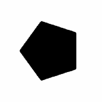
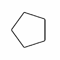
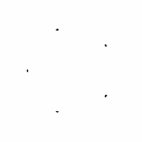
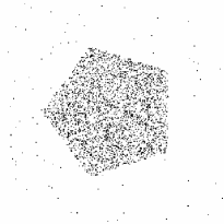
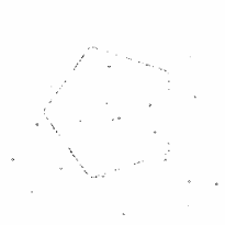
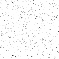
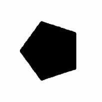
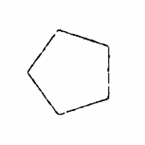
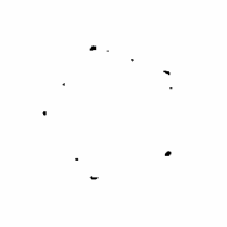
Figure 2: These panels illustrate the application of scale–space operators (see Section 2.1) and geometric invariants (see Section 2.2) to a two–dimensional image. All nine panels were constructed from the image in the top left corner. The first row shows a pentagon and two of the geometric invariants, namely edgeness and cornerness which obviously enhance the corresponding features. In the second row we see the pentagon disturbed by Poissonian noise points of equal strength. Although the pattern is still visible, the geometric invariants – again we show cornerness in the middle column and edgeness in the right column – fail to find the inherent features. However, by applying a scale–space filter of moderate width, we arrive at the series of images shown in the bottom row. Both the original pentagon and its edges and corners as seen by geometric invariants have been reconstructed, although the noise is still present.

2.1 Scale–Space Operators

In order to separate the various scales present in a given field $u_{0}$ we wish to erase structure on scales below a given length $\sigma$, thus arriving at a new field $u_{\sigma}$. In the most general approach, this is done by applying an operator ${\cal G}_{\sigma}$, that is

$$u_{\sigma}={\cal G}_{\sigma}u_{0}.$$ (1)

The precise form of the so–called scale–space operator remains to be specified.

It has been shown by koenderink:geometry (see also the appendix of koenderink:scalespace) that the natural choice for ${\cal G}_{\sigma}$ is the convolution with a Gaussian kernel of width $\sigma$:

$$G_{\sigma}({\bf x},{\bf y})=\frac{1}{(2\pi\sigma^{2})^{d/2}}\exp\left(\frac{||{\bf x}-{\bf y}||^{2}}{2\sigma^{2}}\right).$$ (2)

In order to achieve this uniqueness we require the following simple and actually fairly compelling properties of the operator:

• Additivity and Closure: Iterating two scale–space operators is equivalent to applying a single scale–space operator with an “added” scale; it turns out that only with additivity of the squares, that is $\sigma_{1}\oplus\sigma_{2}=\sqrt{\sigma_{1}^{2}+\sigma_{2}^{2}}$ we can satisfy all requirements simultaneously.

  $${\cal G}_{\sigma_{1}}\circ{\cal G}_{\sigma_{2}}={\cal G}_{\sigma_{1}\oplus\sigma_{2}}.$$ (3)

• Limits: Erasing no structure leaves the image unaltered, while erasing structure on all scales erases the image completely.

  $${\cal G}_{\sigma\rightarrow{0}}={\bf 1}\mbox{ and }{\cal G}_{\sigma\rightarrow\infty}={\bf 0}.$$ (4)

• Linearity: We assume validity of the superposition principle, that is structure on one scale is not influenced by features on another scale. The operator is thus linear and can be expressed as a convolution with an appropriate kernel,

  $$u_{\sigma}({\bf x})=\int{{\rm d}^{d}\!x\,}\int{{\rm d}^{d}\!y\,}G_{\sigma}({\bf x},{\bf y})u_{0}({\bf y}).$$ (5)

• Invariance: Rotational and translational invariance reduce the dependence of the kernel on two points to a dependence on a single scalar, the distance of the points.

  $$G_{\sigma}({\bf x},{\bf y})=G_{\sigma}(||{\bf x}-{\bf y}||).$$ (6)

2.2 Geometric Invariants

$u_{,i}u_{,i}$	edgeness
$u_{,ii}$	profile’s extrema …
$u_{,ii}u_{,jj}-u_{,ij}u_{,ij}$	…and saddlepoints
$u_{,i}u_{,ij}u_{,j}-u_{,i}u_{,i}u_{,jj}$	cornerness

Table 1: This table summarizes a choice of basic invariants that is unique and complete to second order in two dimensions. Furthermore, all invariants may be interpreted as morphometric quantities as given in the right column.

The simplest way to characterize local geometry around a point of the support of a random field is to expand the field as a Taylor series to sufficient order $N$ around this point. The first two orders, and the general expression are

$$\begin{split}u_{\sigma}({\bf x}+{\bf y})&=u_{\sigma,i}({\bf x})y_{i}+{\cal O}(y^{2})\\ u_{\sigma}({\bf x}+{\bf y})&=u_{\sigma,i}({\bf x})y_{i}+\frac{1}{2}u_{\sigma,ij}({\bf x})y_{i}y_{j}+{\cal O}(y^{3})\\ &\vdots\\ u_{\sigma}({\bf x}+{\bf y})&=\sum_{M=0}^{N}\frac{u_{\sigma,i_{1}{\ldots}i_{M}}({\bf x})}{M!}y_{i_{1}}{\ldots}y_{i_{M}}+{\cal O}(y^{N+1}).\end{split}$$ (7)

Obviously, considering the derivatives up to $N$-th order allows us to gain insight into the field’s local behaviour while discarding higher orders in a controlled manner. However, mere derivatives depend on the choice of coordinate system. If we remove these unwanted degrees of freedom by considering coordinate independent invariants such as the square of the gradient instead of its components, we arrive at a description of local geometry that is both complete, in the sense that it contains all information up to $N$-th order, and unique, in the sense that all invariants can be constructed as polynomials in a few basic invariants.

As an important example we will consider a basis for invariants up to second order in two dimensions. By counting degrees of freedom – derivatives of first and second order give five independent numbers, but one of these degrees of freedom is removed when fixing the coordinate system – we conclude that four invariants, apart from the field $u$ itself, can be found. A simple choice is

$$u_{,i}u_{,i}\quad u_{,ii}\quad u_{,i}u_{,ij}u_{,j}\quad u_{,ij}u_{,ji}$$ (8)

Not all of these basic invariants allow for an intuitive interpretation. We have to go to a different, equivalent basis which is summarized in Table 1, together with geometric interpretations. $u_{,i}u_{,i}$ is the square of the gradient and is expected to become large at the steepest edges, hence the term “edgeness”. The quantities $u_{,ii}$ and $u_{,ii}u_{,jj}-u_{,ij}u_{,ji}$ are nothing but the trace and determinant of the Hessian matrix of the field’s profile and thus provide information about the nature of extrema. Finally, $u_{,i}u_{,ij}u_{,j}-u_{,i}u_{,i}u_{,jj}$ is related to the curvature of isolines, which becomes large at corners of the field’s isolines and was accordingly named “cornerness” by koenderink:scalespace.

In Figure 2 we demonstrate the effect of scale–space operators and geometric invariants on a simple pattern.

2.3 Statistical Descriptors

After applying scale–space filters and calculating geometric invariants, we arrive at a field ${\cal I}_{\sigma}$ that contains less unwanted structure for an appropriate choice of $\sigma$ and enhances geometric features according to the invariant that has been chosen. Several possibilities exist to construct statistical descriptors from these fields.

2.3.1 Isodensity contours

The surface integration necessary for the calculation of the genus of isodensity contours [Gott III et al.1986] can be reduced to taking a spatial mean value of Koenderink invariants, multiplied with a delta function for selecting the specific isodensity contour. For the Euler characteristic $\chi=1-g$ of the isodensity contour of the field $u({\bf x})$ to the threshold $\nu$, for example, one obtains

$$\chi(\nu)=\frac{1}{2\pi}\int\!{{\rm d}^{d}\!x\,}\frac{u_{,i}u_{,ij}u_{,j}-u_{,i}u_{,i}u_{,jj}}{u_{,k}u_{,k}}\delta(u-\nu)$$ (9)

Recently, this rationale has been used by schmalzing:beyond to calculate not only the genus, but all Minkowski functionals for a continuous random field in three dimensions.

2.3.2 Excursion sets

It is possible to measure the size of an invariant’s excursion set over its mean value – the sharper the features emphasized by the invariant, the smaller the excursion set. Double Poisson processes for various geometrical objects can be efficiently discriminated by measuring the excursion sets and successively filtering out larger and larger scales in the point distribution (see schmalzing:diplom for further details).

2.3.3 Probability density

Finally, one can think of using the probability density of an invariant as an indicator of certain patterns. It is especially promising to compare the measured curves to analytically calculated mean values for simple types of random fields. We have developed a test for the Gaussianity of random fields and will present preliminary results of its application to CMB anisotropies in the following Section 3.

3 Gaussianity of Random Fields

It is generally believed that the Cosmic Microwave Background anisotropies obey the statistics of a Gaussian random field, at least on scales observed by the COBE satellite. On smaller scales the situation is not so clear. In any case it is important to assess whether there are any non–Gaussian signatures in the microwave sky.

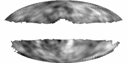
Figure 3: This figure shows a Microwave sky map constructed from the COBE DMR four–year data. By removing the monopole and dipole from the mean value $(A{+}B)/2$ of the 53GHZ channels, the anisotropies on smaller scales become visible. Finally, we only use the 3881 pixels not covered by COBE group’s mask for galactic emission to plot this map and to apply Koenderink invariants.

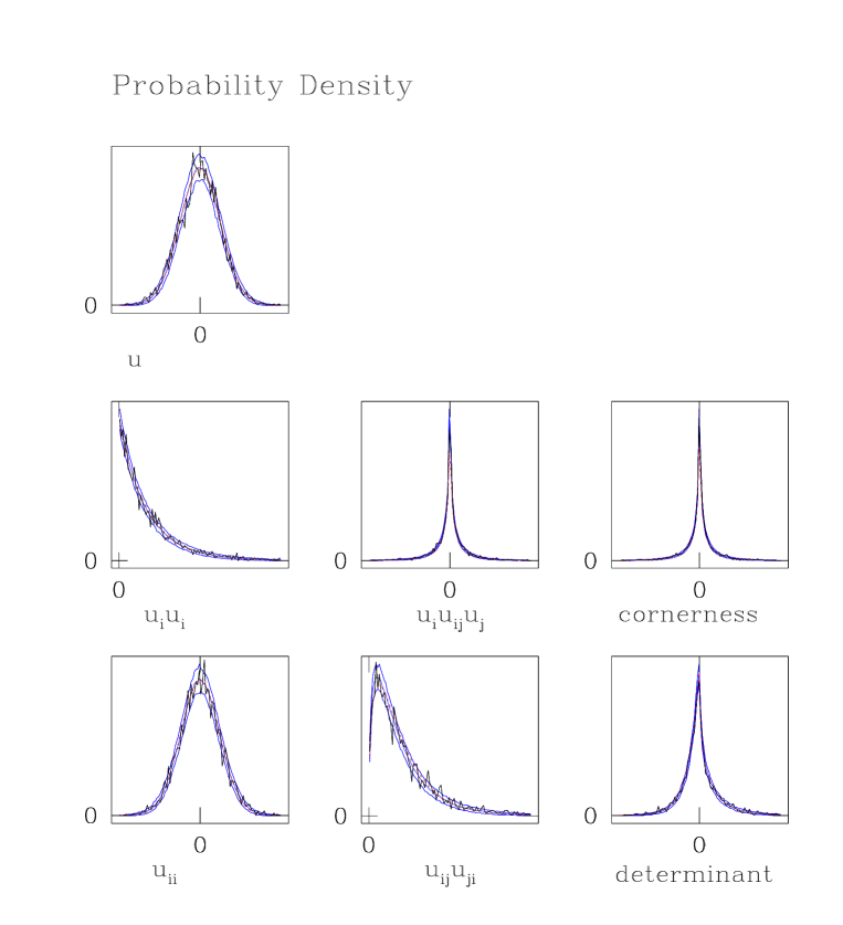
Figure 4: Here we display the results of an analysis of the map in the previous figure. The probability densities of several Koenderink invariants are shown, both as measured from the data (solid line) and as calculated for 100 realizations of a Gaussian random field (the shaded area denotes $1\sigma$ fluctuations).

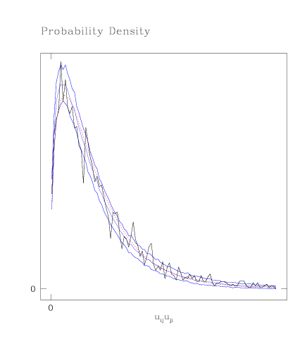
Figure 5: This plot shows the probability density of one of the invariants from Figure 4. The solid, irregular line was measured from the COBE DMR data. The area indicated by the three smoother solid lines corresponds to $1\sigma$–fluctuations calculated from one hundred realizations of a Gaussian random field. Obviously the fluctuations of the data around the fitted mean value (dotted line) are consistent with a Gaussian random field. However, we do see slight discrepancies; future work will assess whether they become significant at higher resolution, when improved statistics reduces the sample–to–sample variance.

3.1 Gaussian Random Fields

The statistical properties of homogeneous and isotropic Gaussian random fields are solely determined by their power spectrum $P(k)$ or equivalently their two–point correlation function $\xi(r)$. Among other works, the standard textbook by adler:randomfields or the article by bardeen:gauss are devoted to an extensive study of random fields in general and Gaussian ones in particular; the calculational schemes presented there also allow to tackle Koenderink invariants of random fields analytically.

3.2 Koenderink Invariants

It turns out that the probability densities of any Koenderink invariant (see schmalzing:diplom for detailed results) depends solely on three common parameters ($\xi(0)$, $\xi^{\prime\prime}(0)$ and $\xi^{\prime\prime\prime\prime}(0)$). Furthermore, they only determine the width of the distribution, while the shape is the same for any Gaussian random field. They can be fitted using the functions measured from the random field, and the goodness of the fit gives a measure of the deviation from Gaussianity.

The panels shown in Figure 4 illustrate the method outlined above. We show a random field, the COBE $(A{+}B)/2$ signal in the 53GHz channel with a customized galactic cut (details can be found in bennett:fouryeardata). From this random field several distribution functions of Koenderink invariants have been calculated. Although the behaviour is largely consistent with the assumption of a Gaussian random field, some deviations are visible. Figure 5 shows and explains one of the seven panels in more detail.

4 Outlook

Apart from the example discussed in this talk, Koenderink invariants suggest a variety of further studies in cosmology.

4.1 Large Scale Structure

The possibility of extending Koenderink invariants to arbitrary dimensions has received only brief attention in this article. On the one hand, Koenderink filters can be used to construct morphological statistics for the three–dimensional matter distribution in the Universe [Schmalzing1996], on the other hand, the insights gained from the theoretical foundations may be used to shed new light on seemingly unrelated measures such as genus statistics [Schmalzing & Buchert1997].

4.2 Microwave Background

The application discussed in this talk uses Koenderink invariants to assess whether non–Gaussian features can be seen in the Cosmic Microwave Background. The preliminary results suggest that this is not the case, at least for the scale probed by the COBE satellite. However, a number of issues remain to be addressed.

Numerical and, if possible, analytical calculations for certain non–Gaussian fields can test the significance of our findings and test the discriminative power in comparison to other methods (e.g. kogut:gaussian).

With regards to the forthcoming high–resolution surveys of the microwave sky [Bersanelli et al.1996, Bennett et al.1995], the performance of Koenderink filters on smaller scales needs to be tested. Their noise reduction abilities are another important subject of study.

Finally, it would be interesting to apply related descriptors other than the probability densities of Koenderink invariants. The methods outlined in Section 2.3 are promising candidates.

References

- [\citefmtAdler1981] Adler, R. J., The geometry of random fields, John Wiley & Sons, Chichester, 1981.
- [\citefmtBardeen et al.1986] Bardeen, J. M., Bond, J. R., Kaiser, N., & Szalay, A. S., Ap. J. 304 (1986), 15–61.
- [\citefmtBennett et al.1995] Bennett, C. L., Hinshaw, G., Jarosik, N. C., Mather, J., Meyer, S. S., Page, L., Skillman, D., Spergel, D. N., Wilkinson, D. T., & Wright, E. L., Bulletin of the American Astronomical Society 187 (1995), 7109+.
- [\citefmtBennett et al.1996] Bennett, C. L., Banday, A., Górski, K. M., Jackson, P. D., Keegstra, P. B., Kogut, A., Smoot, G. F., Wilkinson, D. T., & Wright, E. L., Ap. J. Lett. 464 (1996), L1–L4.
- [\citefmtBersanelli et al.1996] Bersanelli, M., Bouchet, F. R., Efstathiou, G., Griffin, M., Lamarre, J. M., Mandolesi, N., Norgaard-Nielsen, H. U., Pace, O., Polny, J., Puget, J. L., Tauber, J., Vittorio, N., & Volonté, S., COBRAS/SAMBA. A mission dedicated to imaging the anisotropies of the cosmic microwave background. report on the phase A study, European Space Agency, February 1996.
- [\citefmtFerreira & Magueijo1996] Ferreira, P. G. & Magueijo, J. C. R., Phys. Rev. D (1996), submitted, astro-ph/9610174.
- [\citefmtGott III et al.1986] Gott III, J. R., Melott, A. L., & Dickinson, M., Ap. J. 306 (1986), 341–357.
- [\citefmtKoenderink & van Doorn1987] Koenderink, J. J. & van Doorn, A. J., Biol. Cybern. 55 (1987), 367–375.
- [\citefmtKoenderink1984] Koenderink, J. J., Biol. Cybern. 50 (1984), 363–370.
- [\citefmtKogut et al.1995] Kogut, A., Banday, A. J., Bennett, C. L., Hinshhaw, G., Lubin, P. M., & Smoot, G. F., Ap. J. 439 (1995), L29–L32.
- [\citefmtKogut et al.1996] Kogut, A., Banday, A. J., Bennett, C. L., Górski, K. M., Hinshaw, G., Smoot, G. F., & Wright, E. L., Ap. J. Lett. 464 (1996), L29–L34.
- [\citefmtSchmalzing & Buchert1997] Schmalzing, J. & Buchert, T., Ap. J. Lett. (1997), in press, astro-ph/9702130.
- [\citefmtSchmalzing1996] Schmalzing, J., Diplomarbeit, Ludwig–Maximilians–Universität München, 1996, in German, English excerpts available.
- [\citefmtTegmark1996] Tegmark, M., Ap. J. Lett. 464 (1996), L35–L38.
- [\citefmtter Haar Romeny et al.1991] ter Haar Romeny, B. M., Florack, L. M. J., Koenderink, J. J., & Viergever, M. A., in: Lecture Notes in Computer Science, Vol. 511, Springer Verlag, Berlin, 1991, pp. 239–255.
- [\citefmtter Haar Romeny1996] ter Haar Romeny, B. M., 1996, Fourth International Conference on Visualization in Biomedical Computing, http://www.cv.ruu.nl/Publications/ps/tutorial.ps.Z.