Evolutionary models for metal-poor low-mass stars. Lower main sequence of globular clusters and halo field stars

Abstract

We have performed evolutionary calculations of very-low-mass stars from 0.08 to 0.8 $M_{\odot}$ for different metallicites from [M/H]= -2.0 to -1.0 and we have tabulated the mechanical, thermal and photometric characteristics of these models. The calculations include the most recent interior physics and improved non-grey atmosphere models. The models reproduce the entire main sequences of the globular clusters observed with the Hubble Space Telescope over the afore-mentioned range of metallicity. Comparisons are made in the WFPC2 Flight system including the F555, F606 and F814 filters, and in the standard Johnson-Cousins system. We examine the effects of different physical parameters, mixing-length, $\alpha$-enriched elements, helium fraction, as well as the accuracy of the photometric transformations of the HST data into standard systems. We derive mass-effective temperature and mass-magnitude relationships and we compare the results with the ones obtained with different grey-like approximations. These latter are shown to yield inaccurate relations, in particular near the hydrogen-burning limit. We derive new hydrogen-burning minimum masses, and the corresponding absolute magnitudes, for the different metallicities.

We predict color-magnitude diagrams in the infrared NICMOS filters, to be used for the next generation of the HST observations, providing mass-magnitudes relationships in these colors down to the brown-dwarf limit. We show that the expected signature of the stellar to substellar transition in color-magnitude diagrams is a severe blueshift in the infrared colors, due to the increasing collision-induced absorption of molecular hydrogen with increasing density and decreasing temperature.

At last, we apply these calculations to the observed halo field stars, which yields a precise determination of their metallicity, and thus of their galactic origin. We find no evidence for significant differences between the halo field stars and the globular cluster sequences.

Subject headings : stars: Low-mass, brown dwarfs — stars: evolution — stars: globular clusters

1 Introduction

Over the past decade considerable effort, both observational and theoretical, has been directed towards a more accurate determination of the stellar lower main sequence, down to the edge of the sub-stellar domain. Such a determination bears important consequences for our understanding of a wide variety of astrophysical problems, from star formation and stellar structure to galactic formation and evolution. Although the lower main sequence of the disk is relatively well determined since the survey of Monet et al. (1992), the situation is less well defined for the Galactic halo, primarily because of the greater difficulties involved in identifying the halo stars. The task of detecting halo low-mass stars (LMS) and measuring their magnitude is of formidable difficulty with ground-based telescopes. Globular clusters (GCs) have always presented a particular interest for the study of the stellar halo since we can more easily determine their main sequence than for field halo stars. Most of the observations of GCs focussed on the upper main sequence, i.e. the turn-off point, and the red giant branch, for a comparison of this region with theoretical isochrones yields a determination of the age of the clusters, and thus a lower-bound for the age of the Galatic halo. Thanks to the tremendous progress in deep photometry realized recently with the Hubble Space Telescope (HST), which reaches unprecedented magnitude and spatial resolution, the lower main sequence of GCs is now observed nearly down to the hydrogen burning limit. Thanks to the high angular resolution achievable with the HST, accurate photometry is feasible to levels about 4 magnitudes fainter than with ground-based observations, allowing photometry of very faint stars. Several HST observations of globular clusters are now available, spanning a large metallicity-range from solar value to substantially metal-depleted abundances, as will be presented in the next section. The lower main sequence of these clusters is well defined and offers a unique possibility to probe low-mass star evolutionary models for various metallicities down to the hydrogen-burning limit.

In spite of considerable progress in stellar theory - internal structure, model atmospheres and evolution - all the LMS models so far failed to reproduce accurately the observed color-magnitude diagrams (CMD) of disk or halo stars below $\sim 4000$ K, i.e. $\sim 0.4-0.6\,M_{\odot}$, depending on the metallicity. All the models predicted too hot an effective temperature for a given luminosity, i.e. were too blue compared to the observations by at least one magnitude (see e.g. Monet, 1992). Such a disagreement stemed essentially from shortcomings both in the physics of the interior, i.e. equation of state (EOS) and thus mass-radius relationship and adiabatic gradient, and in the atmosphere, since all models were based on grey atmospheres and a diffusion approximation. Important progress has been made recently in this field with the derivation of an appropriate EOS for low-mass stars and brown dwarfs (Saumon, Chabrier & Van Horn 1995; see Chabrier and Baraffe 1997), non-grey model atmospheres for M-dwarfs (Allard and Hauschildt 1995, 1997; Brett 1995) and evolutionary models based on a consistent treatment between the interior and the atmosphere profile (Baraffe, Chabrier, Allard & Hauschildt 1995; Chabrier, Baraffe & Plez 1996; Chabrier & Baraffe, 1997). These models now reach quantitative agreement with the observations, as shown in the afore-mentioned papers and presented in §4.

Globular clusters offer the great advantage of all stars having the same metallicity, determined relatively accurately from bright star spectroscopic measurements. Moreover they are old enough for all the stars to have reached thermal equilibrium, so that age effects do not affect the luminosity of the objects near the bottom of the MS. For these reasons, the mass-luminosity relationship is well determined along the entire MS of GCs, from the turn-off down to the brown dwarf limit, with no dispersion due either to age or metallicity. From the theoretical viewpoint, these properties restrain appreciably the degrees of freedom in the parameter space, so that globular clusters provide a very stringent test to probe the validity of low-mass star evolutionary models and of the related mass-luminosity relationships for various metallicities. Agreement between these models and observations is a necessary condition (but not sufficient !) to assess the validity of these mass-luminosity relationships, a cornerstone to derive reliable mass-functions.

In this paper, we present new evolutionary models for metal-depleted ($[M/H]\leq-1$) low-mass stars ($m\leq 0.8\,M_{\odot}$), based on the most recent non-grey model atmospheres. We compare the results with the observed CMDs of three globular clusters, namely $NGC6397$, $M15$ and $\omega Cen$, for which HST observations are available. The paper is organized as follows : the observations are summarized in §2 whereas the theory is outlined in §3, where comparison is made with other recent LMS models. Comparison between theory and observation is presented in §4. Section 5 is devoted to discussion and conclusion.

The extension of the present calculations to more metal-rich clusters ([Fe/H] $\geq$ -0.5) and field stars, which require more extensive calculations, will be presented in a forthcoming paper (Allard et al. 1997b), as well as the derivation of the mass function for globular star clusters and halo field stars, from the observed luminosity functions (Chabrier & Méra, 1997).

2 Observations

The decreasing luminosity of stars with mass ($L\sim m^{2.5-3.5}$ for low-mass stars) renders the observation of the lower main sequence almost impossible from ground-based telescopes. Despite these difficulties, a number of clusters have been investigated with large telescopes by several groups worldwide to determine the bottom of the main sequence. To our knowledge, the most extensive study was conducted by Richer et al. (1991) who determined accurately the MS of six GCs up to a magnitude $V\sim 24;M_{V}\sim 10$, i.e. a mass $m\sim 0.4\,M_{\odot}$. Although intrinsically interesting, these observations do not provide any information about the very bottom of the MS, and the shape of the luminosity function near the hydrogen-burning limit. Moreover, for metal-depleted abundances, the afore-mentioned limit magnitude and mass correspond to a temperature $T_{\rm eff}\sim 4000$ K (see §4). Above this temperature, the physics of the stellar interiors and atmospheres is relatively well mastered, so that these observations put little constraint on the models, and the related mass-luminosity relationship.

A recent breakthrough in the field has been accomplished with the deep photometry of several GCs obtained with the refurbished Space Telescope. Several observations are now available for $NGC6397$ (Paresce, DeMarchi & Romaniello, 1995; Cool, Piotto & King, 1996), $NGC7078$ ($\equiv M15$) (DeMarchi & Paresce 1995; Piotto, Cool & King, 1996)and $\omega\,Cen$ (Elson, Gilmore, Santiago & Casertano, S., 1995). Observations for these clusters reach $V\sim 27$, $I\sim 24$, almost the very bottom of the main sequence, and thus provide a unique challenge to probe the validity of the LMS models down to the brown dwarf regime.

$\bullet$ Metallicity. All the afore-mentioned clusters are substantialy metal-depleted. Before going any further, it is essential to define what we call ”metallicity” in the present context, for different definitions are used in the literature. What is observed in globular clusters is the iron to hydrogen ratio $[Fe/H]$. The continuous production of oxygen in type II supernovae during the evolution of the Galaxy has led to the well observed enhancement of the oxygen to iron $[O/Fe]$ abundance ratio in old metal-poor stars with respect to the young disk population. Since our basic models assume a solar-mix composition, i.e. $[Fe/O]=0$, the afore-mentioned oxygen-enhancement must be taken into account to make consistent comparison between theory and observation. We use the prescription derived by Ryan and Norris (1991) for halo subdwarfs, i.e.

$$[M/H]\,\approx[O/H]=[O/Fe]\,+\,[Fe/H]$$

with

$$[O/Fe]\,=\,+0.35\,\,\,\,\,\,\,\,\,\,\,{\rm for}\,\,\,[Fe/H]\leq-1$$

$$[O/Fe]\,=\,-0.35\times[Fe/H]\,\,\,\,{\rm for}\,\,-1\leq[Fe/H]\leq 0$$

Thus a cluster with an observed $[Fe/H]=-1.3$, for example, corresponds to a model with a metallicity $[Z]=\log(Z/Z_{\odot})=[M/H]\sim-1.0$, certainly not $[M/H]=-1.3$. This latter choice does not take into account the enhancement of the $\alpha-$elements and yields inconsistent comparisons, especially at the bottom of the MS where the stellar optical spectra and colors are shaped by H^-, MgH, CaH and TiO opacities. The Ryan & Norris correction is based on the spectroscopically-determined abundance of 370 kinematically selected halo stars in the solar neighborhood. Although this procedure is not as fully consistent as calculations conducted with the exact mixture, it certainly represents a fairly reasonable correction for the metal-poor star oxygen enrichment. The accuracy of this prescription will be demonstrated in §3.4, where calculations with the appropriate $\alpha$-enhanced mixture are presented.

$\bullet$ Photometric conversion. The afore mentioned clusters have been observed with the Wide Field and Planetary Camera-2 (WFPC2) of the HST, using either of the $F814W\sim I$, $F555W\sim V$ or $F606W$ filters, where $I,V$ refer to the standard (Johnson-Cousins) filters. Thanks to the courtesy of A. Cool, I. King, G. DeMarchi, F. Paresce, G. Gilmore and R. Elson, we have been able to use the data in these filters, in the so-called WFPC2 Flight system for $NGC6397$, $M15$ and $\omega\,Cen$. For these clusters, comparison between theory and observations is made directly in the Flight system, thus avoiding any possible uncertainties in the synthetic flight-to-ground photometric transformations of Holtzman et al. (1995). The model magnitudes were calculated using the filter transmissions curves and the observed zero points prescribed by Holtzman et al. (1995).

The conversion of apparent $m$ (observation) to absolute $M$ (theory) magnitudes requires the knowledge of the distance modulus ($m-M$), corrected for the interstellar extinction in each filter. In order to minimize the bias in the comparison between theory and observation, we have used the analytical relationships of Cardelli et al. (1989) to calculate the extinctions from the M-dwarf synthetic spectra of Allard & Hauschildt (1997) over the whole frequency-range, from the reddening value $E(B-V)$ quoted by the observers, and we have compared the observed data with the theoretical models corrected for reddening in the WFPC2 filters, when available. The extinction in each filter was found to depend very weakly on the spectral type ($\mathrel{\hbox{\hbox to0.0pt{\lower 2.15277pt\hbox{$\sim$}\hss}\raise 1.72218pt\hbox{$<$}}}0.05$ mag), and thus to be fairly constant over the whole considered temperature range. We believe these determinations, based on accurate synthetic spectra, to yield the most accurate extinction and reddening corrections and the most consistent comparison between theory and observation. These values are given in Table I, for each cluster, and compared to the values quoted by the observers. Table I also summarizes the characteristics adopted for the three clusters of interest. Note that some undetermination remains in the distance modulus of $NGC6397$, yielding a difference in the magnitude of $\sim 0.2$ mag, as will be shown in §4. This stresses the need for a more accurate determination of this parameter.

3 Theory

We have derived recently evolutionary models aimed at describing the mechanical and thermal properties of LMS. These models are based on the most recent physics characteristic of low-mass star interiors, equation of state (Saumon, Chabrier & VanHorn 1995), enhancement factors of the nuclear rates (Chabrier 1997) and updated opacities (Iglesias & Rogers 1996; OPAL), the last generation of non-grey atmophere models (Allard & Hauschildt 1997, AH97) and accurate boundary conditions between the interior and the atmosphere profiles. This latter condition is crucial for an accurate description of LMS evolution, for which any diffusion approximation or grey treatment yield inaccurate results (Baraffe, Chabrier, Allard & Hauschildt 1995; Chabrier, Baraffe and Plez 1996; Chabrier & Baraffe, 1997). A complete description of the physics involved in these stellar models is presented in Chabrier and Baraffe (1997) and we refer the reader to this paper for detailed information.

Below $\sim 0.4\,M_{\odot}$, the stellar interior becomes fully convective : the evolution of LMS below this limit is rather insensitive to the mixing length parameter $\alpha=l/H_{p}$, and thus the models are not subject to any adjustable parameter. From this point of view, VLMS represent a formidable challenge for stellar evolution theory. Comparison with the observations is straightforward and reflects directly the accuracy of the physics and the treatment of the (self-consistent) boundary conditions involved in the calculations. Any VLMS model including an adjustable parameter or a grey atmosphere approximation in order to match the observations would reflect shortcomings in the theory and thus would lead to unreliable results. From this point of view, it is important to stress that, although agreement with the observation is a necessary condition to assess the validity of a stellar model, it is not a sufficient condition. This latter requires the assessment of the accuracy of the input physics and requires parameter-free, self-consistent calculations.

The first generation of the present models (Baraffe et al. 1995) were based on the ”Base” grid of model atmospheres of Allard and Hauschildt (1995; AH95). These models improved significantly the comparison with the observed Pop I and Pop II M-dwarfs sequences (Monet et al. 1992), down to the bottom of the main-sequence, w.r.t. previous models (Baraffe et al. 1995). The AH95 models have been improved recently by including (i) a pressure broadening treatment of the lines, (ii) more complete molecular line lists, and (iii) by extending the Opacity-Sampling technique to the treatment of the molecular line absorption coefficients. This yields the so-called ”NextGen” models ( Allard and Hauschildt 1997). The ”NextGen” synthetic spectra and colors have been compared with Population-I M-dwarf observations by Jones et al. (1995, 1996), Schweizer et al. (1996), Leggett et al. (1996), Viti et al. (1996), and have been used for the analysis of the brown dwarf Gl229B by Allard et al. (1996). The present work is the first application of the ”NextGen” model atmospheres to observations and evolutionary calculations of metal-poor populations.

A first (preliminary) set of the present improved stellar models has been shown to reproduce accurately the observed mass-magnitude (Henry & Mc Carthy 1993) and mass-spectral type (Kirkpatrick & Mc Carthy 1994) relationships for solar-metallicity LMS down to the bottom of the main sequence (Chabrier, Baraffe and Plez 1996; Baraffe & Chabrier 1996). The aim of the present work is to extend the comparison between theory and observation to metal-depleted abundances, characteristic of old disk and halo populations.

For this purpose, we have calculated evolutionary models for masses $m\leq 0.8\,M_{\odot}$ down to the hydrogen-burning limit, based on the ”NextGen” model atmospheres, for different low metal abundances characteristic of old globular clusters, namely $[M/H]=-2,\,-1.5,\,-1.3$ and $-1.0$. This low-metal grid represents a first step towards a complete generation of models covering solar metallicities. A major source of absorption in VLMS arises from the presence of $TiO$ and $H_{2}O$ molecular bands in the optical and the infrared, respectively. Although tremendous progress has been accomplished over the past few years in this type of calculations, some uncertainty remains in the absorption coefficients of these molecules, which affect not only the spectrum, i.e. the colors, but also the profile of the atmosphere, and thus the evolution of late-type M dwarfs (see Allard et al. 1997a for a review of VLM stellar atmospheres modeling). Furthermore, the onset of grain formation, not included in the present models, may also affect the spectroscopic and structural properties of metal-rich VLMS below $T_{\rm eff}\approx 2600$ K (Tsuji et al. 1996a,b; Allard et al. 1996). We expect these shortcomings in the models to be of decreasing importance with decreasing metallicity. Strong double-metal bands ($TiO$, $VO$), for example, are noticeably weaker in the spectra of metal-poor subdwarf (see e.g. Leggett 1992; Dahn et al. 1995), whereas they would dominate the spectrum of a solar metallicity object at this temperature. For this reason it is important to first examine the accuracy of the models for low-metal abundances and its evolution with increasing metallicity. The observed MS of the three afore-mentioned HST GCs represent a unique possibility to conduct such a project.

In some cases, comparison is made with the first generation of models (Baraffe et al. 1995), based on the ”Base” model atmospheres. This will illustrate the effect of the most recent progress accomplished in the treatment of LMS atmospheres. All the basic models assume a mixing length parameter, both in the interior and in the atmosphere, $\alpha=l/H_{P}=1.0$. Since the value of the mixing length parameter is likely to depend to some extent on the metallicity, there is no reason for the value of $\alpha$ in globular clusters to be the same as for the Sun. Although the choice of $\alpha$ is inconsequential for fully convective stars, it will start bearing consequences on the models as soon as a radiative core starts to develop in the interior. For metallicities $[M/H]\leq-1$, this occurs for masses $m\geq 0.4$ $M_{\odot}$ (see Chabrier & Baraffe 1997 for details). In order to examine the effect of the mixing length parameter for masses above this limit, we have carried out some calculations with $\alpha=2$, both in the interior and in the atmosphere (see §3.2 below). All the models assume a solar-mix abundance (Grevesse & Noels 1993). As discussed in the previous section, oxygen-enhancement in metal-poor stars is taken into account by using the eqn.(1) as the correspondence law between solar-mix and $\alpha$-enhanced abundances. In order to test the accuracy of this procedure, a limited set of calculations with the exact $\alpha$-enriched mixture have also been performed (§3.4).

The adopted helium fraction is $Y=0.25$ for all metallicities. The effect of helium abundance will also be examined below.

All models have been followed from the initial deuterium burning phase to a maximum age of 15 10⁹ yr.

Before comparing the results with observations, we first examine some intrinsic properties of the models. Comparison is also made with other recent LMS models for metal-poor stars, namely D’Antona & Mazzitelli (1996; DM96) and the Teramo group of Dr. Castellani (Alexander et al. 1997). Although the EOS used by the Teramo group is the same as in the present calculations (SCVH), both groups use grey model atmospheres based on a $T(\tau)$ relationship, and match the interior and the atmosphere structures either at an optical depth $\tau=2/3$ (DM96) or at the onset of convection (Teramo group).

3.1 Mass-effective temperature relationship

Figure 1 shows the mass-effective temperature relationship for two metallicities, $[M/H]=-1.5$ ($Z=6\times 10^{-4}$) (solid line) and $[M/H]=-1.0$ ($Z=2\times 10^{-3}$)(dash-dot line). We note the two well established changes in the slope at $T_{\rm eff}\approx$ 4500 K and 3800 K, respectively, for these metallicities. The first one corresponds to the onset of molecular formation in the atmosphere, and the related changes in the opacity (see e.g. Copeland, Jensen & Jorgensen 1970; Kroupa, Tout & Gilmore 1990). The second reflects the overwhelming importance of electron degeneracy in the stellar interior near the hydrogen burning limit (DM96; Chabrier & Baraffe 1997). As expected, the enhanced pressures of lower metallicity mixtures yield larger effective temperatures for a given mass (see Chabrier & Baraffe, 1997).

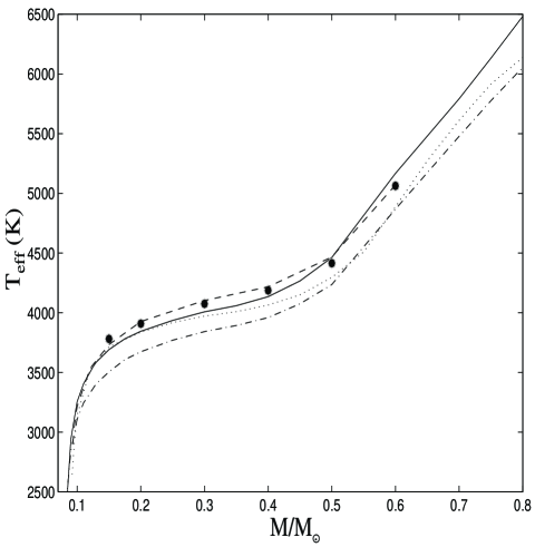
Figure 1: Mass - effective temperature relation for $[M/H]$=-1.5 (solid line) and $[M/H]$=-1.0 (dash-dot line). The full circles denote our calculations done with the Krisha-Swamy grey-like treatment (see text) for $[M/H]$=-1.5 while the dashed line show the results of the Teramo group (Alexander et al., 1997) for the same metallicity. The dotted line shows the results of D’Antona & Mazzitelli (1996; DM96) for $[M/H]$=-1.0.

Also shown on the figure are comparisons with DM96 and the Teramo group, for comparable metallicities. The DM96 models (dotted line) overestimate substantially the effective temperature, by up to $\sim 200$ K below 0.5 $M_{\odot}$. This will yield substantially blue-shifted sequences in the CMDs. This is a direct consequence of using a $T(\tau)$ prescription (and a different EOS, and adiabatic gradient), which implies a grey atmosphere and radiative equilibrium, two conditions which become invalid under low-mass star characteristic conditions, as demonstrated in previous work (Chabrier, Baraffe & Plez 1996; Chabrier & Baraffe 1997). The Krishna-Swamy (1966,KS) formula used by the Teramo group is known to slightly improve this shortcoming. As shown in the figure, we reproduce the Teramo results (dashed line) when using the KS $T(\tau)$ relationship (filled circles). Though smaller, the departure of the mass-$T_{\rm eff}$ relationship in that case is still significant, in particular near the brown dwarf domain, where it becomes too steep and predicts too large hydrogen burning minimum masses (see Chabrier & Baraffe, 1997). A detailed examination of these different prescriptions is given in Chabrier & Baraffe (1997). These comparisons show that, even though some improvement can be reached w.r.t. the basic Eddington approximation, any atmosphere-interior boundary treatment based on a prescribed $T(\tau)$ relation yields incorrect, substantially overestimated, effective temperatures for $T_{\rm eff}\mathrel{\hbox{\hbox to0.0pt{\lower 2.15277pt\hbox{$\sim$}\hss}\raise 1.72218pt\hbox{$<$}}}4500$ K, i.e. $m\mathrel{\hbox{\hbox to0.0pt{\lower 2.15277pt\hbox{$\sim$}\hss}\raise 1.72218pt\hbox{$<$}}}0.5\,M_{\odot}$. Conversely, they underestimate the mass for a given temperature (luminosity) below this limit, i.e. at the bottom of the MS. This illustrates the unreliability of any grey-like treatment to describe accurately the non-grey effects and the presence of convection in optically thin layers of VLM stars. This bears important consequences for the cooling history and thus the evolution in general, and for the mass-luminosity relationship and thus the mass calibration in particular.

3.2 Effect of the mixing length

In this section, we examine the effect of the mixing length parameter $\alpha=l/H_{p}$ on the stellar models, for a given metallicity. We must distinguish the effect of this parameter in the stellar interior and in the atmosphere. Both effects reflect the importance of convective transport in two completely different regions of the star, namely the envelope and the photosphere, and thus do not necessarily bear the same consequences on the models.

We first examine the effect of the mixing length parameter in the atmosphere, by conducting evolutionary calculations with non-grey model atmospheres for [M/H]=-1.5, calculated with $\alpha=1$ and 2, while the value is kept unchanged in the interior. We have selected a range of effective temperatures and gravities ($T_{eff}$ = 4000 - 5800 K, log g = 4.5 - 5) corresponding to masses $m=0.3-0.7$ $M_{\odot}$. The atmosphere profiles corresponding to both situations are shown in Fig. 2, where the onset of convection and the location of the optical depth $\tau$ = 1 are indicated. As seen on the figure, the atmosphere profile is rather insensitive to a variation of $\alpha$ in the optically-thin region, as expected from the rather shallow convection zone in the atmosphere at this metallicity and effective temperature. The main consequence is that the spectrum, and thus the colors and magnitudes at a given $T_{eff}$, remain almost unaffected (less than 0.04 mag in the afore-mentioned range). Below $\sim 3000$ K, the effect of the mixing length in the atmosphere is inconsequential (see also Brett 1995). The evolutionary models calculated with both sets of model atmospheres in the selected range of effective temperatures differ by less than 50 K in $T_{\rm eff}$. The effect of the mixing length in the atmosphere thus bears no consequence on the evolution.

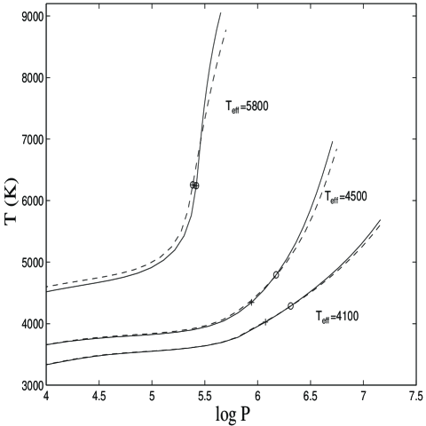
Figure 2: Atmosphere profiles for $[M/H]$=-1.5 and a mixing length $l=H_{P}$ (solid line) and $l=2\,H_{P}$ (dash line), respectively, for selected effective temperatures. The open circles indicate the location of $\tau=1$ and the crosses show the onset of convection.

We now examine the effect of convection in the stellar interior, by conducting calculations with $\alpha=1$ and 2 in the interior, keeping the fiducial value $\alpha=1$ in the atmosphere. This is illustrated in Figure 3a by comparing the solid line (and empty circles), which corresponds to $\alpha=1$ in the interior, with the dashed line (triangles), which corresponds to $\alpha=2$, for $t=10$ Gyr. As expected the effect is null or negligible for convection-dominated interiors, i.e. $m\mathrel{\hbox{\hbox to0.0pt{\lower 2.15277pt\hbox{$\sim$}\hss}\raise 1.72218pt\hbox{$<$}}}0.6\,M_{\odot}$. Above this limit, a larger mixing parameter, i.e. a more efficient convection, yields slightly hotter (bluer) models (D’Antona & Mazzitelli 1994; Chabrier & Baraffe, 1997), about 200-300 K for $T_{\rm eff}=5800-6500$ K, i.e. $m=0.7-0.8\,M_{\odot}$, for the metallicity of interest, $[M/H]=-1.5$.

In summary, the effect of the variation of the mixing length parameter on the stellar models remains weak for the lower MS and is essentially affected by the value in the stellar interior. A variation of $\alpha=1$ to 2 yields variations $\Delta T_{\rm eff}/T_{\rm eff}\sim 2-5\%$ on the effective temperature in the upper MS, for masses above $\sim 0.6\,M_{\odot}$, while the luminosity remains essentially unaffected. We will examine in section 4.1 whether comparison with the observed MS of GCs can help calibrating this value.

3.3 Effect of the age

The effect of the age in a color-magnitude diagram is shown on Figure 3a, for $[M/H]=-1.5$ for ages $t=10$ and 15 Gyr. The time required to reach the zero-age main sequence is much smaller than the age of GCs over the entire stellar mass range so that all hydrogen burning objects do lie on the MS and the bottom of the GC MS is unaffected by age variation. On the other hand, metal-poor stars are significantly hotter and more luminous than their more metal-rich counterparts. Therefore, for a given mass, they burn more rapidly hydrogen in their core, and thus evolve more quickly off the MS. The more massive (i.e. hotter) the star, the larger the effect. This defines the turn-off point, i.e. the top of the MS. For fixed metallicity, the turn-off point will thus be reached for lower masses, i.e. fainter absolute magnitudes, as the age increases. This is illustrated in Figure 3a where we compare the 10 Gyr and 15 Gyr isochrones calculated for different mixing length parameters, for the same metallicity. While the position in the HR diagram of masses below $\sim 0.6\,M_{\odot}$ remains unchanged, larger masses become substantially bluer and more luminous with age as they transform more central hydrogen into helium. The resulting increase of molecular weight yields further contraction and heating of the central layers, and thus an increase of the radiative flux ($F_{rad}\propto T^{3}$) and the luminosity. Eventually they evolve off the MS for a (turn-off)-mass $m_{TO}\sim 0.8\,M_{\odot}$ for $[M/H]=-1.5$ and $-2$ at t=10 Gyr and $m_{TO}\sim 0.75\,M_{\odot}$ at 15 Gyr. As shown on the figure, the upper MS is sensitive to age and mixing length variations. The calibration of the mixing length parameter on the turn-off point is then altered by age uncertainties. The precise determination of the turn-off point thus requires more detailed calculations, which are out the scope of the present study.

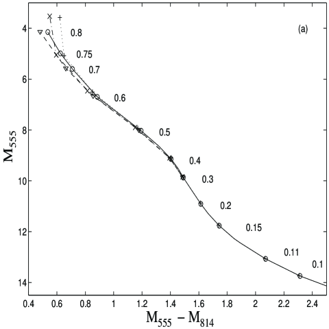
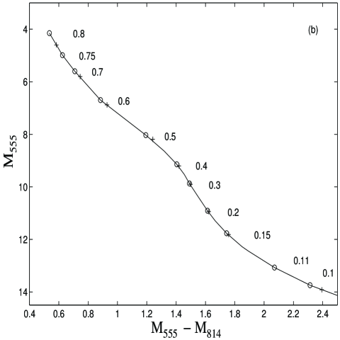
Figure 3: (a) Effect of the age and of the mixing length in the stellar interior for [M/H]=-1.5. The models display the $t=10$ Gyr isochrone when using a mixing length $l=H_{P}$ (solid line; empty circles) and $l=2\,H_{P}$ (dashed line; triangles). The dotted line ($+$) shows the 15 Gyr isochrone calculated with $l=H_{P}$, whereas the dash-dotted curve ($X$) corresponds to t=15 Gyrs and $l=2\,H_{P}$. The masses indicated on the figure correspond to the 10 Gyrs isochrones (open circles and triangles). The upper mass corresponding to the 15 Gyrs isochrones is 0.75 $M_{\odot}$. (b) Effect of the helium fraction $Y$, for $[M/H]=-1.5$, with Y = 0.25 (solid curve, open circles) and Y = 0.23 (+).

3.4 Effect of helium and $\alpha$-elements

As mentioned above, the fiducial calculations have been conducted with a helium abundance $Y=0.25$. Figure 3b compares these results (solid line; circles), for $[M/H]=-1.5$, with calculations done with $Y=0.23$ ($+$). The corresponding variations of the temperature (color) and the luminosity (magnitude) are negligible over the entire mass range, except near the turn-off point.

In order to examine the accuracy of the Ryan & Norris prescription (eqn.(1)), we have conducted calculations using model atmospheres computed with an $\alpha$-element abundance enrichment of $[\alpha/Fe]=0.3$ for a $[Fe/H]=-1.3$ ($[\alpha/H]=-1.0$) mixture. Since the spectra of VLMS near the bottom of the MS are governed by $\alpha$-elements, we expect this mixture to yield equivalent results to those obtained with the scaled-solar abundance mixture of [M/H]= -1.0. This test will also determine whether neglecting a relative under-abundance of $Fe$ and other non-$\alpha$ elements in the scaled-solar abundances does affect or not the shape of the MS. We have computed model atmospheres with the afore-mentioned modified abundances for several temperatures and gravities in the range $T_{\rm eff}=3000-5000$ K and $\log g=4.5-5.0$. We find that the atmosphere density and temperature profiles and the colors are essentially undistinguishable from the ones calculated with $[\alpha/Fe]=0.0$, $[M/H](=[Fe/H])=-1.0$, i.e. a scaled solar-mix, throughout the entire atmosphere.

We have also examined the effect of $\alpha$-enriched abundances in the interior opacities (OPAL), thanks to appropriate opacities kindly provided by F. Rogers for $[M/H]$=-1.0 and $[\alpha/Fe]=0.3$. Here too we find that the effect is negligible and does not modify noticeably the isochrones. This assesses the validity of the Ryan & Norris procedure to take into account the $\alpha$-element enrichment for metal-poor stars, and demonstrates the consistency of our prescription, i.e. comparing solar-mix models with $[\alpha/H]=[M/H]=-1.0$ to observations with $[Fe/H]=-1.3$. Conversely, this demonstrates the inconsistency of comparing observations and solar-mix models for these stars with $[Fe/H]=[M/H]$, as done sometimes in the literature.

The theoretical characteristics of the present models, effective temperature, luminosity, gravity, bolometric magnitude and magnitudes in $VRIJHK$ for several metallicities and an age t = 10 Gyrs are given in Tables II - V.

4 Results and discussion

4.1 Comparison with globular cluster main sequences

Figures 4-6 show the main sequence CMDs of the three GCs mentioned in §2. As mentioned previously, the CMDs are shown in the $M_{555}$ ($\sim V$), $M_{814}$ ($\sim I$), and $M_{606}$ filters in the WFPC2 Flight system to avoid possible errors due to uncertain photometric conversion into the standard Johnson-Cousins system. In all cases, the main sequence is well defined down to $I\approx 25$, $V\approx 27$. Below this limit, the observed MS dissolves into the field and it becomes quite difficult to distinguish the cluster-MS from field stars.

The theoretical MS for the appropriate metallicity, as described in §2, are superimposed to the observations in each figure. For comparison in the $Flight$ system, observed magnitudes have been dereddened with the corrections derived from the synthetic spectra (cf. Table I). The first striking result is the excellent agreement between theory and observation for the three clusters, spanning a fairly large metallicity range from strongly metal-depleted abundances ($M15$) to a tenth of solar metallicity ($\omega\,Cen$). In particular, the changes of the slope in the observed MS are perfectly reproduced by the models, for the correct magnitude, color and metallicity. Since these changes stem from the very physical properties of the stellar interior and atmosphere, as discussed in the previous section, the present qualitative and quantitative agreement assesses the accuracy of the physical inputs in the present theory. The masses corresponding to these changes are indicated on the curves and their effective temperatures are given in Tables II - V, for the various metallicities.

Let us now consider each cluster in turn in order of increasing metallicity.

$\bullet$ $M15$ (Fig. 4a,b) : This is the most metal-depleted HST cluster presently observed, with $[Fe/H]\sim-2.26$ (Djorgovski 1993), i.e. $[M/H]\sim-2.0$ within the prescription adopted in the present paper. The MS of $M15$, as observed by DeMarchi & Paresce (1995), is shown in Figure 4a, with the distance modulus adopted by these authors. Comparison is made with our models with $[M/H]=-1.5$ (solid line) and -2.0 (dashed line). Although both models merge in the upper MS, metallicity effect is clearly reflected in the lower MS where the peak of the spectral distribution falls in the V bandpass, i.e. below $m<0.6\,M_{\odot}$, $M_{606}-M_{814}>0.6$, and $T_{\rm eff}<5000$ K. As seen on the figure, the agreement with the observations over the whole MS is excellent for $[M/H]=-2$ (the observationally-determined metallicity) although the models appear to be slightly too red by $\sim 0.05$ mag or overluminous by $\sim 0.2$ mag, in the upper MS. Even though this discrepancy is within the observational error bars in $m_{606}$ and $m_{814}$, which range from $\pm 0.03$ mag for the upper MS to $\pm 0.17$ mag for the lower MS (DeMarchi, private communication), we will examine the possibilities for this disagreement to be real. A slightly lower metallicity would leave the upper MS almost unchanged, as seen from the two theoretical sequences displayed on the figure. Although the offset in the upper MS might be compensated by a slightly larger mixing length (see §3.2), the fact that it is quite constant along the entire sequence — whereas the mixing length only affects the upper MS (see §3.2) — rather suggests either an overestimated reddening $E(B-V)$ (by $\sim$ 0.05 mag) or an underestimated distance modulus. Indeed, assuming $(m-M)_{814}=15.5$, i.e. $+0.2$ mag w.r.t. the value quoted by DeMarchi & Paresce, or a reddening fainter by $\sim 0.05$ mag would bring theory and observation into perfect agreement. A 0.2 mag error on the distance modulus corresponds to $\sim 1$ kpc, i.e. $\sim$ 10% of the canonical value used presently (Djorgovski 1993). Such an error cannot be excluded for this remote cluster ($D\approx 10.5$ kpc).

Note that we exclude an artificial offset in the calibration of the model magnitudes as source of discrepancy, since we use the magnitude zero-points kindly provided by G. DeMarchi. However, a calibration problem of the data in the $F606W$ filter cannot be excluded, since a disagreement appears as well in the comparison of NGC6397 observed by the same group in the same filters. The disagreement however vanishes for the same cluster in $M_{505}$ and $M_{814}$ and for $wCen$ observed by Elson et al. (1995) in $M_{606}$ and $M_{814}$ (see below). The latter agreement seems to reject an intrinsic problem of the atmosphere models in the spectral region covered by the $M_{606}$ passband.

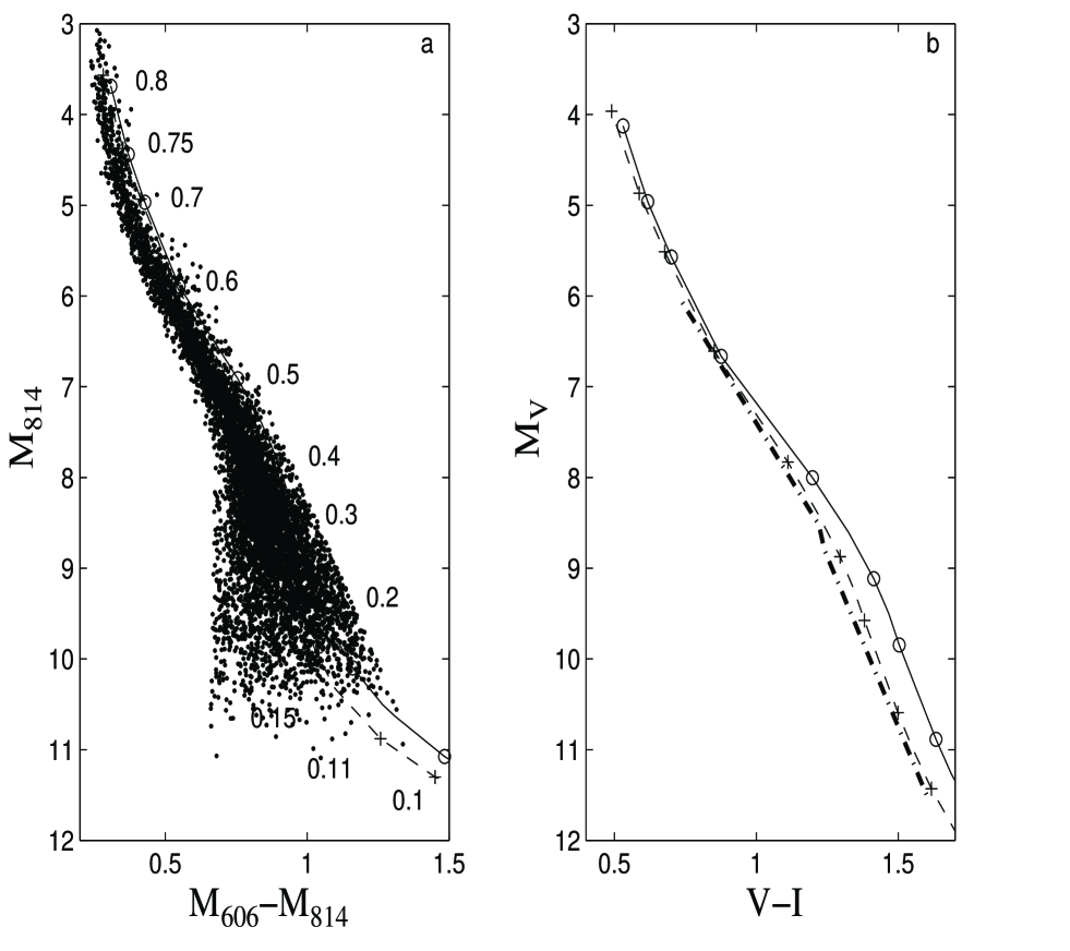
Figure 4: (a) CMD for $M15$. The data in the $606$ and $814$ filters are from DeMarchi & Paresce (1995). The data are dereddened with the corrections calculated in the present study, as given in Table I. Solid line (o): $[M/H]$=-1.5; dashed line (+): $[M/H]$=-2.0. (b) Same as in Fig. 4a in the Johnson-Cousins system with the fit of Santiago et al. (1996) for the cluster (thick dash-dot).

The data of DeMarchi & Paresce have been transformed into the standard $V-I$ Johnson-Cousins system by Santiago et al. (1996) who used the dereddening correction quoted by the former authors (see Table I) and the synthetic transformations of Holtzman et al. (1995). Figure 4b compares the $M15$ MS fit derived by Santiago et al. to the present models in the same Johnson-Cousins color system, where the filter transmissions of Bessell (1990) have been applied to the models. The agreement is similar to that obtained in the previous Flight system, well within the error bars of the photometric $m_{606}$-to-$V_{J}$ transformation, with the same slight offset in color. This comparison assesses the validity of the photometric synthetic transformations of Holtzman et al. (1995) in the present filters.

As shown in the figure and in Table II, the faintest observed stars on the MS, $M_{814}\sim 10$ or $M_{V}\sim 11.5$, correspond to a mass $m\sim 0.15\,M_{\odot}$, still well above the hydrogen burning limit. This latter, $m=0.083\,M_{\odot}$ for $[M/H]=-2$, is expected to correspond to $M_{814}\sim 14.6$, $M_{606}-M_{814}\sim 4.3$ or $M_{V}\sim 21$ and $(V-I)\sim 6.5$ (Table II). At the bright end, the limit of the observations corresponds to the turn-off point $M_{814}\sim M_{I}\sim 3$ (DeMarchi & Paresce 1995) which corresponds to $\sim 0.8\,\pm 0.05\,M_{\odot}$ depending on the age. Note that the Johnson-Cousins fit given by Santiago et al. (1996) starts at $M_{V}\sim 6$, which corresponds to a mass $m\sim 0.6-0.7M_{\odot}$ and does not include the upper MS.

$\bullet$ $NGC6397$ (Fig. 5a,b,c) : This cluster has been observed separately by Paresce et al. (1995) and Cool et al. (1996) in different photometric filters, thus allowing comparison in the three WFPC2 filters mentioned previously. Figure 5a shows the comparison of the observations and the models in $M_{814}$ vs $M_{606}-M_{814}$ for $[M/H]=-1.5$ and $-2$. The best agreement is obtained for the observed metallicity $[M/H]=-1.5$, although admitedly the theoretical sequence lies near the blue edge of the low MS ($M_{814}\mathrel{\hbox{\hbox to0.0pt{\lower 2.15277pt\hbox{$\sim$}\hss}\raise 1.72218pt\hbox{$>$}}}8$). We note however that the error bars for this cluster range from $\pm 0.02$ for the brightest stars to $\pm$ 0.20 mag for the lower MS (cf. Paresce et al. 1995). The agreement displayed in Fig. 5a is therefore well within the error bars. Much better agreement is found in $M_{555}$ vs $M_{555}-M_{814}$, as shown on Figure 5b, although an offset now appears for the intermediate part of the sequence ($M_{555}\sim 8$), $\sim 0.05$ mag in color and $\sim 0.3$ mag in magnitude. As shown on Figure 3a, this part of the MS is insensitive to the mixing length, and the disagreement would thus not be solved by a larger mixing length. In the same vein, models with $\alpha$-enriched abundances would yield similar results, as discussed in §3.4. Models with a substantially lower metallicity would fail reproducing the shape of the MS both in $M_{555}$ (cf. Fig. 5b) and $M_{814}$ (see Fig. 5a).

Fig. 5a

Fig. 5b

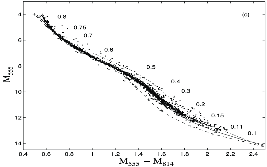
Fig. 5c

Figure 5: (a) CMD for $NGC6397$ in the $606$ and $814$ filters. The data are from DeMarchi & Paresce (1995). The data are dereddened with the corrections calculated in Table I. Solid line (o): $[M/H]$=-1.5; dashed line (+): $[M/H]$=-2.0. The distance modulus is the one quoted by Cool et al. (1995), i.e. $(m-M)_{0}$=11.7. (b) CMD for $NGC6397$ in the $555$ and $814$ filters. The data are from Cool et al. (1995). The data are dereddened with the extinctions calculated in Table I. Dot-dashed line ($\bullet$): stellar models based on the ”Base” model atmospheres (Baraffe et al. 1995) for [M/H]=-1.5; solid line (o): present stellar models based on the ”NextGen” model atmospheres for [M/H]=-1.5; dashed line (+): $[M/H]$=-2.0 with the NextGen model atmospheres. The distance modulus is the same as in Figure 5a, i.e. $(m-M)_{0}$=11.7. (c) Same as figure 5b, with the distance modulus quoted by DeMarchi & Paresce (1995), i.e. $(m-M)_{0}$=11.9 and the same extinction as in Figure 5b. Solid line (o): $[M/H]$=-1.5; dashed line (+): $[M/H]$=-2.0. A comparison with the models of the Teramo group for [M/H]=-1.5 is shown (dash-dot)

Both figures 5a and 5b are displayed with the distance modulus quoted by Cool et al. (1996), i.e. $(m-M)_{0}=11.7$. The choice of the value quoted by Paresce et al. (1995 ), $(m-M)_{0}=11.9$, brings the tracks for $[M/H]=-1.5$ exactly on the observed sequence for the $M_{555}$ vs $M_{555}-M_{814}$ CMD, as illustrated on Figure 5c. Such an undetermination in the distance modulus of $NGC6397$ corresponds to a difference of 200 pc, i.e. about $10\%$. In the $M_{606}$ and $M_{814}$ filters, the models are slightly too blue, with an offset in color $\,\hbox{\hbox{$<$}\kern-8.00003pt\lower 4.30554pt\hbox{$\sim$}}\,0.05$ mag, which can well stem from the same calibration problem in $F606W$ mentioned previously for the cluster M15. The predicted sequence with the metallicity [M/H]=-1.5 remains however well within the error bars of the observed MS.

It is interesting to analyse the agreement obtained by the Teramo group models for this cluster. We first note that their models, while based on a solar-mix, correspond to $[M/H]=[Fe/H]$ rather than $[M/H]=[O/H]$. As discussed in the previous section, this leads to inconsistent comparisons, and is reflected by the fact that: i) they fit the MS with a rather low value of the metallicity for this cluster ($-1.9<[M/H]<-1.6$), and ii) they adopt a reddening correction $E(V-I)=0.19$ which differs significantly from the value prescribed by Cool et al. (1996) and by the present calculations (see Table I). Using the correct extinction would redshift significantly their models for [M/H]=-1.5 w.r.t. the observations, as shown on Fig. 5c (dash-dotted line).

Note that for this cluster, the observations are still above the hydrogen-burning limit. The HBMM $\sim 0.083\,M_{\odot}$ corresponds to $M_{V}\sim 19.5$, $M_{I}\sim 13.9$ for $[M/H]=-1.5$, whereas the bottom of the observed MS, $M_{V}\sim 13$, $M_{I}\sim 11$, corresponds to $m=0.11\,M_{\odot}$. The observations of Cool et al. (1996) extend to brighter magnitudes and reach the turn-off point, $M_{V}\sim 4$, $m\sim 0.8\,\pm 0.05\,M_{\odot}$.

A limited set of the first generation of the present models at $[M/H]=-1.5$, based on the ”Base” model atmospheres (Baraffe et al. 1995), is also shown on Figure 5b for $m\leq 0.2\,M_{\odot}$ (full circles, dash-dot line). These models have a slightly different trend w.r.t. the present ones. This stems from a general overestimation of the molecular blanketing, the main source of absorption in the coolest VLMS, because of the straight-mean approximation in the ”Base” models, and thus an underestimation of the flux in the V-band ( Chabrier et al. 1996; Allard & Hauschildt 1997). The better agreement with the present models clearly illustrates the recent improvements in the treatment of the molecular opacities, especially for $TiO$ (AH97), which strongly affect the atmosphere profile, and thus the evolution. However, the agreement between the previous models and observations was already quite satisfactory ($\sim 0.2$ mag) and for the first time reproduced accurately the bottom of the observed MS for metal-poor LMS.

$\bullet$ $\omega-Cen$ (Fig. 6) : this cluster has been observed by Elson et al. (1995) in the F606W and F814W filters. The observed metallicity usually quoted for this cluster is $[Fe/H]\sim-1.6$, i.e. $[M/H]\sim-1.3$ (cf Elson et al. 1995 and references therein), although a value $[Fe/H]\sim-1.2$, i.e. $[M/H]\sim-1.0$ has been suggested recently (Norris et al., 1996). The data presented in Figure 6 have been recalibrated (Elson, private communication), since the calibrations of Holtzmann et al. (1995) used in Elson et al. (1995) were preliminary at this time. The zero points for both HST filters are updated (cf. Holtzmann et al. 1995), as well as the transformation into the Johnson-Cousins system. Here again, the match between theory and observation is almost perfect, as shown in Figure 6, in both the HST instrumental and the Jonhson-Cousins systems. Note that both systems predict the same masses for the upper MS ($m\sim 0.75M_{\odot}$) and the lower MS ($m\sim 0.15M_{\odot}$), well within the error bars due to the photometric conversion from $m_{606}$ into $V_{J}$ (Holtzman et al. 1995). Once again, this assesses the accuracy of the present photometric conversions of HST magnitudes into Johnson-Cousins magnitudes.

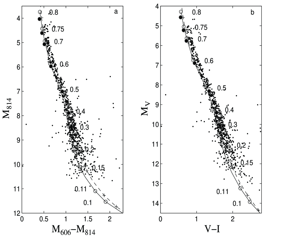
Figure 6: (a) CMD for $\omega-Cen$. The data in $606$ and $814$ filters are from Elson et al. (1995). The models correspond to [M/H]=-1.3 (solid line, open circle) and [M/H]=-1.0 (dashed line, $+$) with $l=H_{P}$. Full circles correspond to [M/H]=-1.0 and $l=2H_{P}$ (b) CMD for $\omega-Cen$ in the Johnson-Cousins system. The data from Elson et al. (1995) have been recalibrated with updated transformations (Elson, private communication). Same models as in (a).

We used the same distance modulus as Elson et al. (1995), i.e. $(m-M)_{0}=13.77$. Adopting the slightly higher value $13.92$ quoted by Santiago et al. (1996) will shift the blue edge of the observed MS on the theoretical isochrone with [M/H]=-1.3, yielding a less good agreement. Our reddening corrections (cf. Table I) are in excellent agreement with the values quoted by Elson et al. (1995). Calculations with a mixing length $l=2H_{P}$ for the [M/H]=-1 isochrone are also shown in Figure 6. Note that the observations remain compatible with a value $1\mathrel{\hbox{\hbox to0.0pt{\lower 2.15277pt\hbox{$\sim$}\hss}\raise 1.72218pt\hbox{$<$}}}l/H_{P}\mathrel{\hbox{\hbox to0.0pt{\lower 2.15277pt\hbox{$\sim$}\hss}\raise 1.72218pt\hbox{$<$}}}2$. Since the same remark applies to the lower-metallicity clusters analysed previously, it would be hazardous to try to derive robust conclusions about a possible dependence of the mixing length on metallicity. The observed width of the lower MS does not allow a precise determination of the metallicity of the cluster from the theoretical isochrones. The shape of the MS is well reproduced with both [M/H]=-1.3 and -1. This result is consistent with the spread in metallicity determined by Norris et al. (1996).

The properties of the models for the afore-mentioned different metallicities, in particular the mass-color-magnitude relationships, are displayed in Tables II-V. The lowest mass in the table corresponds to the hydrogen-burning minimum mass (HBMM) for each metallicity. For an age $t=$ 10 Gyr and metallicities [M/H] $\leq-1.0$, the magnitude of the most massive brown dwarf is $\sim$2 mag in $I$ and $K$, $\sim$3 mag in $V$ and $\sim 1.5$ mag in $J$ and $H$ fainter than the one corresponding to the HBMM. This sets the scale of the detection limit for the search for brown dwarfs in globular clusters with future space-based observations.

As already mentioned and clearly seen from the figures and from Tables II - V, the more metal-depleted clusters have bluer main sequence colors, a consequence of the increasing effective temperature at a given mass with decreasing metallicity, since the same optical depth corresponds to a denser layer in an increasingly transparent atmosphere (see e.g. AH95; Chabrier & Baraffe 1997). Metallicity effects are most apparent in the intermediate MS, i.e. $m\,\hbox{\hbox{$<$}\kern-8.00003pt\lower 4.30554pt\hbox{$\sim$}}\,0.5\,M_{\odot}$ and $T_{\rm eff}\,\hbox{\hbox{$<$}\kern-8.00003pt\lower 4.30554pt\hbox{$\sim$}}\,4500$ K, where the peak of the spectral distribution falls near the V bandpass. This stems essentially from the increasing TiO-opacity, which absorbs mainly in the optical and reddens the $(V-I)$ color. Thus, for a given $T_{\rm eff}$, a metal poor object will appear bluer than the more metal-rich counterpart. This effect is strengthened at fixed mass by the fact that the lower the metallicity, the hotter (bluer) the star.

4.2 Color-magnitude diagram in the near infrared

The observations of GCs in near IR colors will soon be possible with the next generation of HST observations, i.e. the NICMOS camera, and in a more remote future, with the european Very-Large-Telescope (VLT). The NICMOS filters include Wide (W), Medium (M) and Narrow (N) bandpasses from 1.1 to 2.4 $\mu$m. In figures 7a-b we show our models at t=10 Gyrs for [M/H]=-2, -1.5 and -1.0 in the NICMOS wide filters F110W, F160W and F187W. For comparison, the same isochrones are displayed in the J ($\sim 110W$) and H ($\sim 160W$) magnitudes (cf. Fig. 7a, dotted curves), defined in the CIT system (Leggett 1992). The masses listed in Table II-V are indicated by the signs ($+$ and circles) on the curves (except 0.13 $M_{\odot}$ excluded for sake of clarity). We note the ongoing competition, in these infrared colors, between the reddening due to the decreasing temperature and increasing metallic molecular absorption in the optical and the increasing collision-induced absorption of H₂ in the infrared (cf. Saumon et al., 1994; Allard & Hauschildt, 1995) which shifts back the flux to shorter wavelengths. This leads to quasi-constant color sequences from $\sim 0.5$ to $\sim 0.1$ $M_{\odot}$, corresponding to $T_{\rm eff}\sim 4500$ K, for which H₂ becomes stable in the atmosphere, to $\sim 3500$ K, as predicted also for zero-metallicity (Saumon et al., 1994). Below this limit, molecular hydrogen becomes dominant, the density keeps increasing ( cf. Chabrier & Baraffe, 1997) and H₂ CIA-absorption becomes the dominant effect ($\kappa_{CIA}\approx\kappa_{H_{2}-H_{2}}\,\rho_{H_{2}}^{2}$ in first order, see Guillot et al., 1994). This causes the blue loop at the very bottom of the MS in IR colors, as seen in Figures 7, whereas the optical colors redden monotonically with decreasing mass, as shown in the tables. The blue loop becomes more dramatic with decreasing metallicities, since the lower the metallicity the denser the atmosphere. This general trend is very similar in all NICMOS filters covering the above-mentioned wavelength range and is clearly a photometric signature of the stellar to sub-stellar transition, whose physical source is the large increase of the density in this region and the ongoing H₂ molecular recombination and collision-induced absorption. The limit magnitudes required to reach the very bottom of the MS are $\sim 14$ for [M/H]=-2, $\sim 12.5$ for [M/H]=-1.5 and $\sim 12$ for [M/H]=-1, and are essentially the same for all NICMOS filters from F110 to F240. The more massive brown dwarfs will be about 2 magnitudes fainter.

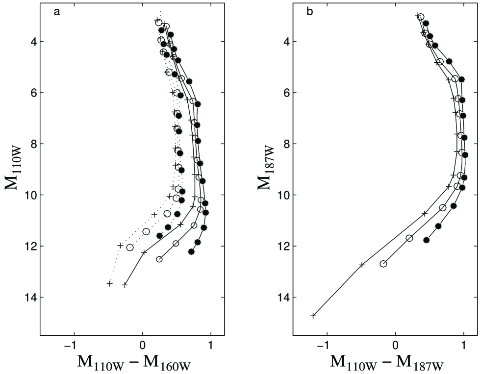
Figure 7: (a) Isochrones at t=10 Gyrs in the NICMOS filters (solid curves) F110W and F160W for three different metallicity [M/H]=-2, -1.5 and -1 (from left to right). The dotted curves correspond to the same isochrones in the CIT system $M_{J}$-(J-H). The signs on the curves correspond to the masses (except 0.13 $M_{\odot}$) tabulated in Tables II to V. (b) Same as in Fig. 7a in the NICMOS filters F110W and F187W.

4.3 Comparison with the halo subdwarf sequence

Figure 8 displays different observations of halo field stars in the standard Johnson-Cousins system. The filled circles are the subdwarf sequence of Monet et al. (1992), the crosses the more complete subdwarf sequence of Dahn et al. (1995), and the triangles correspond to a sub-sample of Leggett’s (1992) halo stars. The halo classification was determined photometrically (Leggett 1992) and kinematically : the stars in the three afore-mentioned samples have tangential velocities $|V_{tan}|>220$ km.s^-1 (Monet et al.), $>$160 km.s^-1 (Dahn et al.) and $>$180 km.s^-1 (present sub-sample of Leggett). All these observations appear to be fairly consistent, the Monet et al. sample representing the most extreme halo fraction of the Dahn et al. sample, the Leggett’s sample containing only a few genuine halo stars. We stress that the linear fit proposed by Leggett (1992) is a rather poor representation of the distribution of the true halo objects and is strongly misleading. We also emphasize that linear fits are not correct to fit LMS sequences in the HR diagram, since they do not reproduce the wavy behaviour of the sequences, wich reflects intrinsic physical properties of these stars, as discussed in §3.1. This non linearity has already been stressed for the mass-luminosity (D’Antona & Mazzitelli, 1994; Chabrier et al., 1996) and the mass-spectral class relations (Baraffe & Chabrier, 1996). We first note the important spread in color, over 1 mag, which reflects the large spread in metallicity in the sample.

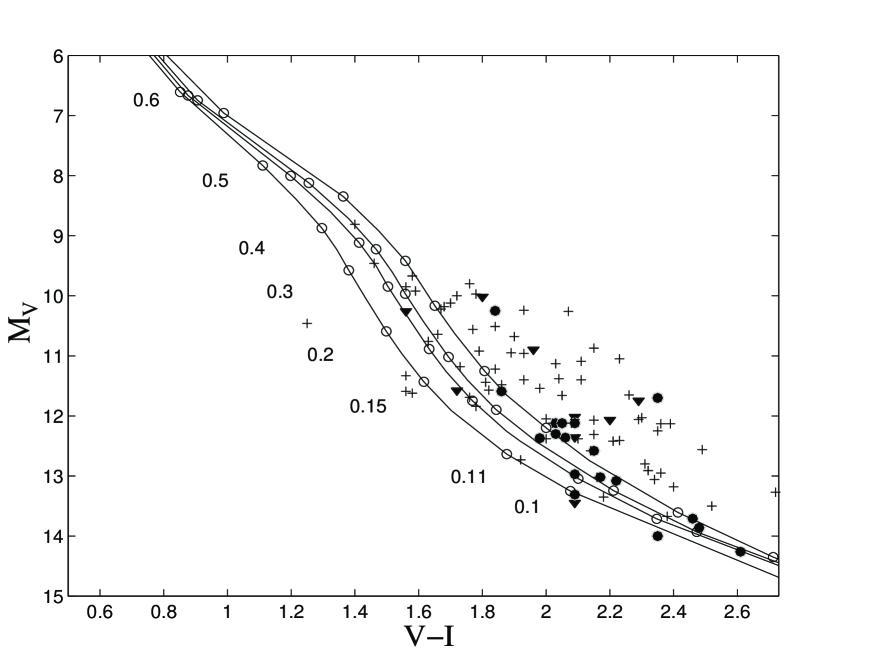
Figure 8: Subdwarf halo field stars from the data of Monet et al. (1992) (full circles), Dahn et al. (1995) ($+$) and Leggett (1992) (triangles), in the standard Jonhson-Cousins system. All the stars shown here from the Leggett’s sample have tangential velocities $|V_{tan}|\geq 180$ km.s^-1. Solid lines: present models for $[M/H]$=-2,-1.5, -1.3 and -1 (from left to right) for t=10 Gyr. The empty circles correspond to the masses indicated on the figure.

The solid lines indicate the present LMS sequences for $[M/H]=-2.0,\,-1.5,\,-1.3$ and -1.0 from left to right. The Monet et al. sample is consistent with an average metallicity $[M/H]\sim-1.3$ to $-1.5$. It is more hazardous to try to infer an average value for Leggett’s sample, given the limited number of objects and the large dispersion. The Dahn at al. sample clearly includes the two previous ones, with objects ranging from $[M/H]\sim-0.5$ to $[M/H]=-2.0$. This reflects the difficulty to determine the precise origin of an object from its kinematic properties only.

As seen on the figure, these field stars are fairly consistent with the theoretical sequences determined for the clusters, for similar metallicities. This is particularly obvious for the sequences of $NGC6397$ ([M/H]=-1.5) and $\omega\,Cen$ ([M/H]=-1.3), which match perfectly the Monet et al. average sequence. This strongly suggests, contrarily to what has been suggested by Santiago et al. (1996), that there is no significant difference in the structure and the evolution of globular star clusters and field halo stars. The discrepancy between the CMD of Leggett (1992) and those from the HST led Santiago et al. (1996) to invoke the possibility of a calibration problem of the HST data. However, the agreement that we find between our theoretical models and the globular cluster CMDs in both the HST data and the Johnson-Cousins system (e.g for $M15$ and $wCen$), excludes this hypothesis. It rather stems form the large metallicity dispersion in Leggett’s sample and from the misleading fit of this sample.

5 Conclusion

We have presented extensive calculations of VLMS evolution in the range $-2.0\leq[M/H]\leq-1.0$, characteristic metallicities for old globular star clusters and halo field stars. These low-metallicities minimize possible shortcomings of the model atmospheres pertaining to incomplete or inaccurate metallic molecular line lists and grain formation, and provide a stepping stone towards the derivation of more accurate low-mass star models for solar metallicity. The models are examined against available deep photometry color-magnitude diagrams obtained with the Hubble Space Telescope for three globular clusters. The HST CMDs for the clusters span a large range in metallicity, thus providing very stringent tests for the models. Since the parameters characteristic of these clusters, extinction, distance modulus and metallicity are fairly well defined, there is no free parameter left to bring models into agreement with observations. Therefore comparison between theory and observation reflects directly the accuracy of the theory. We stress the importance of eqn.(1) when comparing GC observed and theoretical CMDs. A first generation of the present models (Baraffe et al. 1995) has been used incorrectly by comparing observations at $[Fe/H]$ with a model at the same value of $[M/H]$.

The main conclusions of these calculations can be summarized as follows :

$\bullet$ We first note the overall remarkable agreement between the present models and the observations, within less than 0.1 mag, over the whole metallicity range and the entire main sequence from the turn-off to the bottom. The characteristic changes in the slopes of the cluster MS’s are reproduced accurately, and assess the validity of the physics involved in the models. This yields an accurate calibration of the observations, i.e. reliable mass-magnitude-effective temperature-age relationships.

We also provide reddening corrections based on accurate LMS synthetic spectra.

$\bullet$ Variations of the mixing length in the stellar interior affect essentially the upper main sequence near the turn-off, i.e. only stars massive enough to develop a large radiative core ($m\mathrel{\hbox{\hbox to0.0pt{\lower 2.15277pt\hbox{$\sim$}\hss}\raise 1.72218pt\hbox{$>$}}}0.7\,M_{\odot}$). Variations of the mixing length in the atmosphere is found to be inconsequential on evolutionary models. There is no clear hint for a dependence of the mixing length on the metallicity and our results remain in agreement with all observed sequences, within the error bars, for $1\leq l_{mix}/H_{P}\leq 2$.

$\bullet$ The Ryan & Norris (1991) prescription to convert solar-mix abundances into oxygen-enriched mixtures characteristic of old stellar populations is accurate. Using the correct $\alpha$-enhanced mixture (both in the atmosphere and in the interior opacities) leads to results identical to those obtained with the afore-mentioned scaling. Not taking this enrichment into account leads to inconsistent comparisons.

$\bullet$ We derive theoretical sequences in the filters of the NICMOS camera, down to the hydrogen burning limit. This will allow a straightforward analysis of the future HST observations, and provides a stringent test for the accuracy of the present models near the brown dwarf limit. This corresponds to $M_{J}\approx M_{H}\approx M_{K}\approx 13-14$ for the lowest metallicity examined presently, i.e. $[M/H]=-1.0$.

We also predict a photometric signature of the transition from stellar to substellar objects in the infrared, in terms of a severe blue loop near the very bottom of the MS, whereas optical colors keep reddening almost linearly. This photometric signature reflects the overwhelming absorption of molecular hydrogen in the infrared due to many-body collisions, and stems from the increase of the molecular hydrogen fraction and of the density (contraction) near the stellar to substellar transition.

$\bullet$ The models allow a good determination of the metallicty of the observed halo field stars. A striking result is the large metallicity dispersion of these objects, from $[M/H]$ = -2 to near solar, although they all have halo kinematic properties. The most extreme halo stars, represented by the Monet et al. (1992) sample, have a metallicity ranging from $[M/H]\sim-1.0$ to -2.0, with an average value $[M/H]\sim-1.3$. We find no evidence for differences in the sequences of halo field subdwarfs and globular star clusters. Both are reproduced with the same isochrones for similar mean metallicity, $[M/H]\sim-1.3$ to $-1.5$, i.e. $[Fe/H]\sim-1.6$ to $-1.8$.

We can now affirm that the theory of low-mass stars, at least for metal-depleted abundances, has reached a very good level of accuracy and can be used with confidence to analyse the observations and make reliable predictions. While we cannot honestly exclude the possibility of a discrepancy in the $M_{606}-M_{814}$ color predicted by the models (by $\sim 0.05$ mag), it remains within the error bars due to the observations themselves and to the undeterminations of either the extinction or the distance modulus. It may also reflect present uncertainties in the calibration of the $F606$ filter.

While it is unfortunate that the hydrogen burning limit remains unreached by the present HST observations, for it is masked by foreground field stars, the next cycles of HST observations will be able to resolve it in the near future. Indeed, known proper motion of the GCs will cause a substantial displacement of cluster stars between 1994 and 1997 which should allow a separation of cluster from field stars (King 1995). Also, as mentioned above, observations in the IR should lead to the observation of the very bottom of - and possibly below - the MS. The present models provide the limit magnitudes to be reached to enter the brown dwarf regime.

The present calculations represent an important improvement in the description of the mechanical and thermal properties of low-mass stars, and of their photometric signature. This provides solid grounds to extend these calculations into the more complicated domain of solar-like metallicities, as will be examined in a forthcoming paper (Allard et al., 1997b). The assessed accuracy of the present models provide reliable mass-luminosity relationships for metal-poor stellar populations in general and for globular clusters in particular. This allows for the first time the derivation of reliable mass-functions for these objects down to the brown dwarf limit (Chabrier and Méra, 1997).

Tables II-V are available by anonymous ftp:

ftp ftp.ens-lyon.fr

username: anonymous

ftp $>$ cd /pub/users/CRAL/ibaraffe

ftp $>$ get BCAH97_models

ftp $>$ quit

Table I: Characteristics of the globular clusters. $[Fe/H]$ is the observed metallicity, $[M/H]$ is the metallicity used in the models, which takes into account the $\alpha$-enrichment following the prescription of Ryan & Norris (see §2). The fourth and fifth columns denote the bare distance modulus and reddening repectively, as quoted by the refered observers. The last three columns give the extinction in the three respective filters $F555\sim V_{J}$, $F606$ and $F814\sim I_{C}$, where $J$ and $C$ denote the standard Johnson-Cousins system. The upper rows give the value chosen by the refered observers whereas the lower rows denote the value used in the present calculations, deduced from the Allard & Hauschildt (1997) synthetic spectra and the Cardelli et al. (1989) extinction law. In all cases the interstellar extinction corresponds to $R_{V}=3.12$.

$cluster$	$[Fe/H]$	$[M/H]$	$(m-M)_{0}$	E(B-V)	$A_{555}$	$A_{606}$	$A_{814}$
M151,2	-2.3	-2.0	15.10	0.11	0.34	0.274	0.144
			15.10	0.11	0.33	0.30	0.20
NGC63973	-1.9	-1.5	11.70	0.18	0.57		0.34
NGC63974	-1.9	-1.5	11.90	0.18			0.30
			11.7 (11.9)	0.18	0.57	0.51	0.35
$\omega$ Cen5	-1.6	-1.3/-1.0	13.77	0.116	0.36	0.32	0.22
			13.77	0.116	0.36	0.33	0.22

¹ Piotto et al. 1995

² De Marchi & Paresce 1995

³ Cool et al., 1996

⁴ Paresce et al. 1995

⁵ Elson et al. 1995

Table II: Physical properties and absolute magnitudes of low-mass stars for $[M/H]=-2.0$ and $\tau$ = 10 Gyrs. The lowest mass corresponds to the hydrogen-burning limit. The mass $m$ is in $M_{\odot}$, $T_{eff}$ in K and the luminosity L in $L_{\odot}$. The VRI magnitudes are in the Johnson-Cousins system (Bessell 1990) and the JHK magnitudes in the CIT system (Leggett 1992). Note that the bolometric magnitude corresponds to $M_{bol}(\odot)$ = 4.64.

$m$	$T_{eff}$	log L	log g	$M_{bol}$	$M_{V}$	$M_{R}$	$M_{I}$	$M_{J}$	$M_{H}$	$M_{K}$
0.083	1779.	-4.274	5.58	15.33	20.92	16.92	14.41	13.47	13.95	14.58
0.085	2342.	-3.741	5.53	13.99	17.67	15.17	13.11	11.98	12.30	12.61
0.090	3005.	-3.202	5.45	12.65	14.70	13.40	11.96	10.77	10.60	10.68
0.100	3395.	-2.860	5.37	11.79	13.25	12.22	11.17	10.06	9.66	9.58
0.110	3565.	-2.686	5.32	11.36	12.63	11.66	10.76	9.69	9.24	9.12
0.130	3749.	-2.463	5.26	10.80	11.91	10.99	10.21	9.20	8.72	8.58
0.150	3852.	-2.306	5.21	10.40	11.43	10.55	9.81	8.84	8.36	8.20
0.200	4004.	-2.020	5.12	9.69	10.59	9.78	9.09	8.17	7.69	7.52
0.300	4172.	-1.665	5.01	8.80	9.58	8.83	8.19	7.33	6.85	6.69
0.400	4304.	-1.421	4.94	8.19	8.87	8.18	7.58	6.75	6.29	6.13
0.500	4623.	-1.083	4.83	7.35	7.83	7.25	6.72	5.99	5.55	5.43
0.600	5292.	-0.676	4.73	6.33	6.61	6.17	5.76	5.20	4.84	4.77
0.700	5914.	-0.265	4.58	5.30	5.51	5.17	4.83	4.40	4.10	4.07
0.750	6282.	-0.015	4.47	4.68	4.87	4.57	4.28	3.90	3.64	3.63
0.800	6688.	0.334	4.25	3.81	3.96	3.72	3.47	3.17	2.95	2.96

Table III: Same as in Table 2 for $[M/H]=-1.5$

$m$	$T_{eff}$	log L	log g	$M_{bol}$	$M_{V}$	$M_{R}$	$M_{I}$	$M_{J}$	$M_{H}$	$M_{K}$
0.083	2194.	-3.844	5.51	14.25	19.42	16.32	13.87	12.06	12.24	12.42
0.085	2519.	-3.559	5.48	13.54	17.50	15.20	13.05	11.43	11.38	11.53
0.090	2938.	-3.207	5.42	12.66	15.21	13.78	12.13	10.73	10.37	10.37
0.100	3255.	-2.910	5.34	11.92	13.71	12.61	11.37	10.13	9.63	9.52
0.110	3405.	-2.745	5.30	11.50	13.04	12.02	10.94	9.77	9.25	9.10
0.130	3586.	-2.523	5.24	10.95	12.25	11.29	10.38	9.28	8.75	8.57
0.150	3691.	-2.366	5.20	10.56	11.75	10.81	9.98	8.93	8.40	8.21
0.200	3845.	-2.082	5.11	9.84	10.89	10.00	9.25	8.26	7.74	7.55
0.300	4008.	-1.724	5.00	8.95	9.85	9.03	8.34	7.42	6.91	6.72
0.400	4134.	-1.471	4.92	8.32	9.11	8.35	7.70	6.82	6.31	6.14
0.500	4462.	-1.116	4.80	7.43	8.00	7.36	6.80	6.01	5.51	5.39
0.600	5167.	-0.702	4.72	6.40	6.66	6.21	5.79	5.20	4.81	4.75
0.700	5792.	-0.296	4.58	5.38	5.57	5.21	4.87	4.42	4.11	4.08
0.750	6132.	-0.059	4.47	4.79	4.96	4.65	4.34	3.95	3.67	3.66
0.800	6483.	0.266	4.27	3.98	4.12	3.86	3.59	3.26	3.02	3.02

Table IV: Same as in Table 2 for $[M/H]=-1.3$

$m$	$T_{eff}$	log L	log g	$M_{bol}$	$M_{V}$	$M_{R}$	$M_{I}$	$M_{J}$	$M_{H}$	$M_{K}$
0.083	2283.	-3.751	5.49	14.02	19.24	16.30	13.83	11.81	11.82	11.95
0.085	2542.	-3.524	5.46	13.45	17.61	15.32	13.12	11.34	11.15	11.25
0.090	2903.	-3.214	5.40	12.68	15.47	13.98	12.23	10.74	10.31	10.27
0.100	3200.	-2.931	5.34	11.97	13.93	12.79	11.46	10.16	9.63	9.49
0.110	3343.	-2.769	5.29	11.56	13.24	12.20	11.03	9.81	9.26	9.09
0.130	3512.	-2.552	5.23	11.02	12.44	11.46	10.47	9.33	8.77	8.58
0.150	3624.	-2.392	5.19	10.62	11.90	10.95	10.05	8.97	8.42	8.22
0.200	3780.	-2.107	5.10	9.91	11.02	10.11	9.32	8.30	7.77	7.57
0.300	3945.	-1.747	4.99	9.01	9.97	9.12	8.41	7.46	6.94	6.74
0.400	4067.	-1.492	4.92	8.37	9.22	8.42	7.76	6.85	6.33	6.16
0.500	4377.	-1.139	4.79	7.49	8.12	7.44	6.86	6.04	5.51	5.39
0.600	5068.	-0.727	4.71	6.46	6.75	6.27	5.84	5.22	4.81	4.74
0.700	5686.	-0.326	4.58	5.46	5.64	5.27	4.92	4.44	4.12	4.09
0.750	6006.	-0.099	4.47	4.89	5.05	4.72	4.41	3.99	3.71	3.69
0.800	6315.	0.199	4.29	4.14	4.29	4.00	3.72	3.36	3.11	3.10

Table V: Same as in Table 2 for $[M/H]=-1.0$

$m$	$T_{eff}$	log L	log g	$M_{bol}$	$M_{V}$	$M_{R}$	$M_{I}$	$M_{J}$	$M_{H}$	$M_{K}$
0.083	2359.	-3.660	5.45	13.79	19.10	16.42	13.93	11.60	11.35	11.42
0.085	2550.	-3.492	5.43	13.37	17.81	15.58	13.31	11.26	10.89	10.91
0.090	2840.	-3.231	5.38	12.72	15.94	14.35	12.44	10.75	10.24	10.15
0.100	3107.	-2.967	5.32	12.06	14.35	13.15	11.64	10.21	9.63	9.46
0.110	3245.	-2.808	5.28	11.66	13.61	12.52	11.19	9.87	9.28	9.09
0.130	3406.	-2.593	5.22	11.12	12.74	11.74	10.61	9.39	8.81	8.60
0.150	3505.	-2.439	5.18	10.74	12.20	11.23	10.20	9.04	8.46	8.25
0.200	3674.	-2.150	5.10	10.02	11.25	10.33	9.45	8.37	7.82	7.60
0.300	3841.	-1.787	4.99	9.11	10.17	9.28	8.51	7.52	6.98	6.78
0.400	3959.	-1.530	4.91	8.46	9.42	8.57	7.86	6.91	6.38	6.18
0.500	4235.	-1.185	4.78	7.60	8.35	7.60	6.98	6.11	5.55	5.42
0.600	4867.	-0.782	4.69	6.60	6.96	6.42	5.97	5.28	4.81	4.74
0.700	5478.	-0.392	4.58	5.62	5.81	5.41	5.04	4.52	4.17	4.13
0.750	5776.	-0.181	4.49	5.09	5.25	4.89	4.56	4.10	3.79	3.77
0.800	6055.	0.077	4.34	4.45	4.59	4.27	3.96	3.56	3.28	3.27