Structure and evolution of low-mass stars

Abstract

We present extensive calculations of the structure and the evolution of low-mass stars in the range 0.07-0.8 $M_{\odot}$, for metallicities $-2.0\leq[M/H]\leq 0.0$. These calculations are based on the most recent description of the microphysics characteristic of these dense and cool objects and on the lattest generation of grainless non-grey atmosphere models. We examine the evolution of the different mechanical and thermal properties of these objects as a function of mass and metallicity. We also demonstrate the inaccuracy of grey models and $T(\tau)$ relationships under these conditions. We provide detailed tables of the mass-radius-luminosity-effective temperature relations for various ages and metallicities, aimed at calibrating existing or future observations of low-mass stars and massive brown dwarfs. We derive new hydrogen-burning minimum masses, within the afore-mentioned metallicity range. These minimum masses are found to be smaller than previous estimates, a direct consequence of non-grey effects.

At last, we examine the evolution of the abundance of light elements, $Li,Be$ and $B$, as a function of age, mass and metallicity.

1 Introduction

Accurate modelling of the mechanical and thermal properties of very-low-mass stars (VLMS), or M-dwarfs, defined hereafter as objects with masses below $\sim$0.8$M_{\odot}$, is of prior importance for a wide range of physical and astrophysical reasons, from the understanding of fundamental problems in basic physics to astrophysical and cosmological implications. VLMS are compact objects, with characteristic radii in the range $0.1\mathrel{\hbox{\hbox to0.0pt{\lower 2.15277pt\hbox{$\sim$}\hss}\raise 1.72218pt\hbox{$<$}}}R/R_{\odot}\mathrel{\hbox{\hbox to0.0pt{\lower 2.15277pt\hbox{$\sim$}\hss}\raise 1.72218pt\hbox{$<$}}}0.7$. Their central densities and temperatures are respectively of the order of $\rho_{c}\approx 10-10^{3}$ g cm^-3 and $T_{c}\approx 10^{6}-10^{7}$ K, so that correlation effects between the particles dominate the kinetic contribution in the interior stellar plasma. Effective temperatures of VLMS are below $T_{eff}\approx 5000$ K, and surface gravities $g=GM_{\star}/R_{\star}^{2}$ are in the range $\log g\approx 3.5-5.5$. These conditions show convincingly that the modelling of VLMS requires a correct description of non-ideal effects in the equation of state (EOS) and the nuclear reaction rates, and a derivation of accurate models for dense and cool atmospheres, where molecular opacity becomes eventually the main source of absorption. Several ground-based and space-based IR missions are now probing the VLMS wavelength range ($\lambda\approx 1-10\,\mu$) down to the end of the main-sequence (MS), reaching sometimes the sub-stellar domain. These existing or future surveys will produce a substantial wealth of data, stressing the need for accurate theroretical models. Indeed the ultimate goal of VLMS theory is an accurate calibration of observations, temperature, luminosity and above all the mass, with the identification of genuine brown dwarfs. At last, VLMS represent the major component ($>70\%$) of the stellar population of the Galaxy. A correct determination of the contribution of these objects to the Galactic mass budget, both in the central parts and in the outermost halo, requires the derivation of reliable mass functions for VLMS, and thus accurate theoretical mass-luminosity relationships for various metallicities.

Tremendous progress has been realized within the past decade in the field of VLMS, both from the observational and theoretical viewpoints. From the theoretical point of view, the most recent benchmarks in the theory, without being exhaustive, have been made by D’Antona & Mazzitelli (1985, 1994), who initiated the research in the field, the MIT group (Dorman, Nelson & Chau 1989; Nelson, Rappaport & Joss 1986, 1993) and the Tucson group (Lunine et al. 1986; Burrows, Hubbard & Lunine 1989; Burrows et al. 1993). So far, all these models, however, failed to reproduce the observations at the bottom of the VLMS sequence, predicting substantially too large temperatures for a given luminosity (see e.g. Monet et al. 1992). This shortcoming of the theory made a reasonable identification of the observational H-R diagram elusive. Such a discrepancy stemed from incorrect stellar radii (and adiabatic gradients), a consequence of inaccurate EOS, but most importantly from the use of grey atmosphere models. These points will be largely examined in §2.4 and §2.5. A significant breakthrough in the structure and evolution of VLMS was made recently by the Tucson group, who first derived evolutionary models based on non-grey atmosphere models (Saumon et al. 1994), although for zero-metallicity, and by the Lyon group (Baraffe et al. 1995, BCAH95; 1997, BCAH97; Chabrier et al. 1996) who derived evolutionary models based on the Allard-Hauschildt (1995a, AH95; 1997, AH97) non-grey model atmospheres for various finite metallicities. The BCAH95 models were shown to improve significantly the afore-mentioned discrepancy at the bottom of the MS. These initial calculations have now been improved substantially. The aim of the present paper is to present a complete description of the physics entering the theory of VLMS and to relate the properties of these objects to well understood physical grounds. Extensive comparisons with available observations, color-magnitude diagrams and mass-magnitude relationships, will be presented in companion papers (BCAH97; Allard et al. 1997a).

The present paper is organized as follows. In §2, we describe the input physics which enters the present theory, EOS, enhancement factors of the nuclear reaction rates, atmosphere models and boundary conditions. Evolutionary models are presented in §3, together with the prediction of the abundances of light elements (⁷Li,⁹Be,¹¹B) along evolution and the burning minimum masses for these elements. We also derive a new limit for the hydrogen burning minimum mass (HBMM), i.e. the brown dwarf limit, which is found to be lower than previous estimates, a direct consequence of non-grey effects. The mass-dependence of photospheric quantities is examined in §4. Section 5 is devoted to the concluding remarks.

2 Input physics

The Lyon evolutionary code has been originally developped at the Göttingen Observatory (Langer et al. 1989; Baraffe and El Eid, 1991 and references therein) and is based on one-dimensional implicit equations of stellar structure, solved with the Henyey method (Kippenhahn and Weigert, 1990). Convection is described by the mixing-length theory. Throughout the present paper, we use a mixing length equal to the pressure scale height, l_mix = H_p as a reference calculation. As discussed in §3.2, the choice of this parameter is inconsequential for the evolution of objects below $\sim 0.6\,M_{\odot}$. For larger masses, the dependence of the results on the mixing length is examined in BCAH97, along comparison with observations. The updated Livermore opacities (OPAL, Iglesias & Rogers 1996) are used for the inner structure ( T $>$ 10 000K). The effect of the improved OPAL opacities compared to the previous generation (Rogers & Iglesias, 1992) on the evolution of VLM stars (BCAH95; Chabrier, Baraffe & Plez 1996) is found to be negligible, affecting the effective temperature by less than 1% and the luminosity by less than 3% for a given mass. For lower temperatures, we use the Alexander and Fergusson (1994) opacities. The helium fraction in the calculations is Y=0.275 for solar-like metallicities and Y=0.25 for metal-depleted abundances.

An adequate theory for stellar evolution requires i) an accurate EOS, ii) a correct treatment of the nuclear reaction rates, iii) accurate atmosphere models and iv) a correct treatment of the boundary conditions between the interior and the atmophere profiles along evolution. Each of these inputs is discussed in the following sub-sections.

2.1 The equation of state

Interior profiles of VLMS range from $\sim 4000$ K and $\sim 10^{-6}$ g cm^-3 at the base of the photosphere (defined as $R_{ph}=\sqrt{(L/4\pi\sigma T_{eff}^{4})}$) to $\sim 10^{7}$ K and $\sim 100$ g cm^-3 at the center for a 0.6 $M_{\odot}$ star, and from $\sim 2800$ K and $\sim 10^{-5}$ g cm^-3 to $\sim 5\,10^{6}$ K and $\sim 500$ g cm^-3 for a 0.1 $M_{\odot}$, for solar metallicity. Within this temperature/density range, molecular hydrogen and atomic helium are stable in the outermost part of the stellar envelope, while most of the bulk of the star (more than 90% in mass) is under the form of a fully ionized H⁺/He⁺⁺ plasma. Therefore a correct EOS for VLMS must include a proper treatment not-only of temperature-ionization and dissociation, well described by the Saha-equations in an ideal gas, but most importantly of pressure-ionization and dissociation, as experienced along the internal density/temperature profile, a tremendously more complicated task. Moreover, under the central conditions of these stars, the fully ionized hydrogen-helium plasma is characterized by a plasma coupling parameter $\Gamma=(Ze)^{2}/akT\propto(Z^{2}/A^{1/3})\,(\rho_{6}^{1/3}/T_{8})\approx 0.5-5$ for the classical ions ($a$ is the mean inter-ionic distance, $A$ is the atomic mass and $\rho$ the mass-density) and by a quantum coupling parameter $r_{s}=<Z>^{-1/3}a/a_{0}=1.39/(\rho/\mu_{e})^{1/3}\approx 0.1-1$ ($a_{0}$ is the electronic Bohr radius and $\mu_{e}^{-1}={<Z>\over<A>}$ the electron mean molecular weigth) for the degenerate electrons. These parameters show that both the ions and the electrons are strongly correlated. A third characteristic parameter is the so-called degeneracy parameter $\psi=kT/kT_{F}\approx 3\times 10^{-6}\,T\,(\mu_{e}/\rho)^{2/3}$, where $kT_{F}$ is the electron Fermi energy. The classical (Maxwell-Boltzman) limit corresponds to $\psi\rightarrow+\infty$, whereas $\psi\rightarrow 0$ corresponds to complete degeneracy. The afore-mentioned thermodynamic conditions yield $\psi\approx 2-0.1$ in the interior of VLMS along the characteristic mass range, implying that finite-temperature effects must be included to describe accurately the thermodynamic properties of the correlated electron gas. At last, the Thomas-Fermi wavelength $\lambda_{TF}=\bigl{(}kT_{F}/(6\pi n_{e}e^{2})\bigr{)}^{1/2}$ (where $n_{e}$ denotes the electron particle density) is of the order of the mean inter-ionic distance $a$, so that the electron gas is polarized by the ionic field, and electron-ion coupling must be taken into account in the plasma hamiltonian. Such a detailed treatment of strongly correlated, polarisable classical and quantum plasmas, plus an accurate description of pressure partial ionization represent a severe challenge for theorists. Several steps towards the derivation of such an accurate EOS for VLMS have been done since the pioneering work of Salpeter (1961) and we refer the reader to Saumon (1994) and Saumon, Chabrier and VanHorn (1995) for a review and a comparison of the different existing EOS for VLMS. In the present calculations, we use the Saumon-Chabrier (SC) EOS (Saumon 1990; Chabrier 1990; Saumon & Chabrier 1991, 1992; Saumon, Chabrier & VanHorn 1995; SCVH), specially devoted to the description of low-mass stars, brown dwarfs and giant planets. This EOS presents a consistent treatment of pressure ionization and includes significant improvements w.r.t. previous calculations in the treatment of the correlations in dense plasmas. This EOS is tied to available Monte Carlo simulations and high-pressure shock-wave experimental data (see SCVH and references therein for details). As shown in Saumon (1994) and SCVH, significant differences exist between the SC EOS and other VLMS EOS, for the pressure-density relations and for the adiabatic gradients, so that we expect substantial differences in the derived stellar radii and entropy profiles. The SCVH EOS has been used previously to derive interior models for solar (Chabrier et al. 1992; Guillot et al. 1995) and extrasolar (Saumon et al. 1996) giant planets and for brown dwarfs (Burrows et al. 1993).

The SC EOS is a pure hydrogen and helium EOS, based on the so-called additive-volume-law (AVL) between the pure components (H and He). The accuracy of the AVL has been examined in detail by Fontaine, Graboske & VanHorn (1977). The invalidity of the AVL to describe accurately the thermodynamic properties of the mixture is significant only in the partial ionization region (see e.g. SCVH). As mentioned above, this concerns only a few percents of the stellar mass under LMS conditions. Given the negligible number-abundance of metals in stars ($\sim 2\%$ by mass, i.e. $\sim 0.2\%$ by number) we expect the presence of metals to be inconsequential on the EOS. Their contribution to the perfect gas term is just proportional to the number density ($P_{id}=\Sigma_{i}N_{i}kT/V$), i.e. $\sim 0.2\%$, whereas their non-ideal (correlation) contribution can be estimated either by the Debye-Huckel correction ($P_{c}\propto(\Sigma_{i}N_{i}Z_{i}^{2})^{3/2}$) for $\Gamma<1$ or by the electrostatic (ion-sphere) term ($P_{c}\propto\Sigma_{i}N_{i}Z_{i}^{5/3}$) for $\Gamma>1$. For solar metal-abundance (see e.g. Grevesse & Noels, 1993) this yields an estimated contribution to the EOS of $\sim 1\%$ compared with the hydrogen+helium contribution.

Although this simple estimation shows that metals do not contribute appreciably to the EOS of VLMS, as long as the structure and the evolution are concerned, we have decided to conduct complete calculations by comparing models derived with the SC EOS and models based on the so-called MHD EOS (Hummer & Mihalas, 1988; Mihalas, Hummer & Däppen, 1988), which includes the contribution of heavy elements under solar abundances. Although the MHD EOS is devoted to stellar envelopes and weakly correlated plasmas, like the solar interior ($\Gamma\sim 0.1$), and thus can not be applied to VLMS, it provides a useful tool for the present test. The test is even strengthened by comparing the complete MHD EOS with the pure hydrogen-helium ($Z=0$) MHD EOS kindly provided by W. Däppen. Note that the MHD EOS for mixtures does not assume the additive-volume law between the various components, so that comparison with this EOS provides also a test for the validity of this approximation.

Figure 1 shows in a HR diagram the results obtained with the MHD EOS for solar metallicity (open circles) and for $Z=0$ (triangles) up to 1 $M_{\odot}$ . The difference is less than 1% in $T_{eff}$ and 4% in L. This demonstrates convincingly the negligible contribution of the metals to the EOS over the entire LMS mass range. As shown above, the contribution of metals to the EOS is proportional to a power of the charge $Z$ and the atomic mass $A$. Therefore, when applying a metal free EOS to solar metallicity objects, the presence of metals can be mimicked by an equivalent helium fraction $Y^{\prime}=Y+Z$ in the EOS, at fixed hydrogen abundance. Varying X instead of Y would yield larger differences in $T_{eff}$ and $L$. Figure 1 also displays results based on the SC EOS, with the afore-mentioned equivalent helium fraction (filled circles). Both the SC and MHD EOS yield very similar results. The differences between the SC and the complete ($Z=Z_{\odot}$) MHD EOS amount to less than 1.3% in $T_{eff}$ and 1% in $L$. Below 0.3 $M_{\odot}$, however, the track based on the MHD EOS starts to deviate substantially from the one based on the SC EOS, a fairly reasonable limit for an EOS primarily devoted to solar conditions.

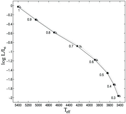
Figure 1: Theoretical HR-diagram for solar metallicity at t=5 Gyrs. Filled circles (solid line) Saumon-Chabrier EOS (SCVH, 1995) with $Y\prime=Y+Z$; triangles (dotted line): metal free (Z=0) MHD EOS with $Y\prime=Y+Z$; open circles : solar metallicity ($Z=Z_{\odot}$) MHD EOS (Mihalas et al. 1988).

This is better illustrated in Figure 2, which displays the adiabatic gradient along the density-profile in a 0.2 $M_{\odot}$ and a 0.6 $M_{\odot}$ star for the SC and MHD EOS. For the 0.6 $M_{\odot}$ star, slight discrepancies between the SC and MHD adiabatic gradient appear in the regime of partial ionisation of hydrogen and helium (log $\rho$ $\approx$ -4 to -0.5 and log T $\approx$ 4.2 to 5.3 ). The differences become substantial for the 0.2 $M_{\odot}$ star because of the strong departure from ideality in a large part of the interior. The main discrepancies appear for log $\rho\mathrel{\hbox{\hbox to0.0pt{\lower 2.15277pt\hbox{$\sim$}\hss}\raise 1.72218pt\hbox{$>$}}}-3~{}g\,cm^{-3}$, with log T $\approx 4$ and $\Gamma\approx~{}2-3$, which marks the onset of hydrogen pressure and temperature partial ionisation. The unphysical negative value of the adiabatic gradient in the MHD EOS for log $\rho>~{}-1$ clearly illustrates the invalidity of the MHD EOS to describe the interior of dense systems, as clearly stated by its authors (see Hummer & Mihalas, 1988). Similar discrepancies occur also for other LMS EOS (see Saumon 1994; SCVH), which will affect substantially the structure and the evolution of these convective objects. We emphasize the excellent agreement between both EOS in the domain of validity of the MHD EOS, even though the SC EOS does not include heavy elements. This clearly demonstrates the negligible effect of metals on the adiabatic gradient. This latter is essentially determined by hydrogen and helium pressure- and temperature- ionisation and/or molecular dissociation.

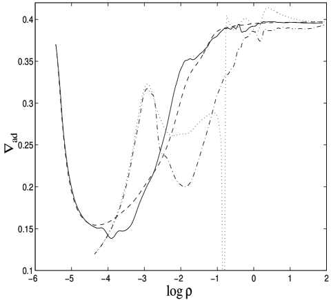
Figure 2: Adiabatic gradient as a function of density for the structure of a 0.6 $M_{\odot}$ (solid and dashed curves) and 0.1 $M_{\odot}$ (dash-dot and dotted curves). The solid and dash-dotted curves correspond to the Saumon-Chabrier EOS (SCVH, 1995). The dashed and dotted curves to the MHD (1988) EOS.

These calculations clearly demonstrate that metal-free EOS can be safely used to describe the structure and the evolution of LMS with a solar abundance of heavy elements, providing the use of an effective helium fraction to mimic the effect of metals. It also assesses the validity of the Saumon-Chabrier EOS, devoted primarily to dense and cool objects, for solar-like masses.

2.2 The nuclear reaction rates

The thermonuclear processes relevant from the energetic viewpoint under the central temperatures and densities characteristic of VLMS are given by the PPI chain :

$$p+p\rightarrow d+e^{+}+\nu_{e}$$

$$p+d\rightarrow^{3}He\,+\,\gamma$$

$${}^{3}He+^{3}He\rightarrow^{4}He\,+\,2p$$

The destruction of ${}^{3}He$ by reaction (3) is important only for T $>6\times 10^{6}$ K i.e masses M $\mathrel{\hbox{\hbox to0.0pt{\lower 2.15277pt\hbox{$\sim$}\hss}\raise 1.72218pt\hbox{$>$}}}0.15\,M_{\odot}$ for ages $t<$ 10 Gyrs, since the lifetime of this isotope against destruction becomes eventually smaller than a few Gyrs. In the present calculations, we have also examined the burning of light elements, namely Li, Be and B, whose abundances provide a powerfull diagnostic to identify the mass of VLMS and brown dwarfs (see §3.3). Our nuclear network includes the main nuclear-burning reactions of ${}^{6}Li,^{7}Li,^{7}Be,^{9}Be,^{10}B$ and ${}^{11}B$ (cf. Nelson et al. 1993). We will focus on the depletion of the most abundant isotopes ${}^{7}Li,^{9}Be$ and ${}^{11}B$, described by the following reactions :

$${}^{7}Li\,+p\,\rightarrow\,2\,^{4}He$$

$${}^{9}Be\,+\,p\,\rightarrow\,d\,+\,2\,^{4}He$$

$${}^{11}B\,+\,p\,\rightarrow\,3\,^{4}He$$

The rates for these reactions are taken from Caughlan and Fowler (1988). These rates correspond to the reactions in the vacuum, or in an almost perfect gas where kinetic energy largely dominates the interaction energy. As already mentioned, such conditions are inappropriate for VLMS. In dense plasmas, the strongly correlated surrounding particles act collectively to screen the bare Coulomb repulsion between two fusing particles. This will favor the reaction and then enhance substantially the reaction rate with respect to its value in the vaccuum. As mentioned in §2.1, under the central conditions characteristic of low-mass stars, the electrons are only partially degenerate and are polarized by the ionic field. This responsive electronic background will also screen the nuclear reactions and must be included in the calculations. Under the conditions of interest, both enhancement factors, ionic and electronic, are of the same order, i.e. a few units (Chabrier 1997). Different treatments of these enhancement factors have been derived, again following the pioneering work of Salpeter (1954). A complete treatment of the ionic screening contribution over the whole stellar interior density-range, from the low-density Debye-Huckel limit to the high-density ion-sphere limit was first derived by DeWitt et al. (1973) and Graboske et al. (1973). The inclusion of electron polarisability, in the limit of strongly degenerate electrons, i.e. $r_{s}\rightarrow 0$ and $\psi\rightarrow 0$, was performed by Yakovlev and Shalybkov (1989). An improved treatment of the ionic factor, and the extension of the electron response to finite degeneracy, as found in the interior of VLMS, was performed recently by Chabrier (1997). The difference between the Graboske et al. and the Chabrier results, which illustrates both the improvement in the calculation of the ionic factor and the effect of electron polarisability, is shown on Figure 3 along temperature profiles characteristic of VLMS, for two central densities, for Li-burning ($Z_{1}=1,Z_{2}=3$). Substantial differences appear, in particular in the intermediate-screening regime ($\Gamma\sim 1-10$) characteristic of LMS and BD interiors. The larger the charge, the larger the effect ($H\propto\Gamma\propto Z_{1}Z_{2}$). Such differences translate into differences in the abundances as a function of time and mass, as will be examined in §3.3. Note that the inclusion of electron polarisability was found to decrease substantially the deuterium-burning minimum mass (Saumon et al. 1996).

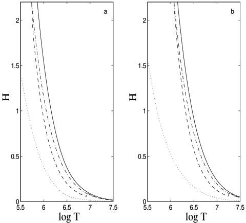
Figure 3: Screening factors as a function of temperature for Lithium-burning (eqn. (4)), for (a) $\rho=10$ g cm^-3 and (b) $\rho=100$ g cm^-3. Solid line : present ion+electron screening factors (Chabrier, 1997); dash-dot : ionic factor only; dot : electron factor only; dashed line : Graboske et al. (1973).

2.3 Deuterium-burning on the main sequence

The initial D-burning phase ends after $\sim 10^{6}$ yrs and is inconsequential for the rest of the evolution and the position on the Main Sequence (Burrows, Hubbard & Lunine, 1989 and §3 below). We focus in this section on the deuterium production/destruction rate along the PPI reactions, given by eqn. (1) and (2), which is essential for the nuclear energy generation required to reach thermal equilibrium. For stars below $M\mathrel{\hbox{\hbox to0.0pt{\lower 2.15277pt\hbox{$\sim$}\hss}\raise 1.72218pt\hbox{$<$}}}0.3\,M_{\odot}$, which are entirely convective (see §3.2), the deuterium lifetime against proton capture $\tau_{pd}$ is found to be much smaller than the mixing timescale in the central regions, where energy production takes place. The mixing time in these regions is estimated from the mixing- length theory (MLT), $\tau_{mix}\approx l_{mix}/v_{mix}$, where $v_{mix}\propto(\nabla-\nabla_{ad})^{1/2}$ is the mean velocity of turbulent eddies. These fully convective stars are essentially adiabatic throughout most of their interior, with a degree of superadiabaticity $(\nabla-\nabla_{ad})$ variing from $\sim$ 10^-8 to $\sim 10^{-3}$ from the center to 99% of the mass. Thus the mixing-length parameter is inconsequential, and a reasonable estimate for the mixing length is the pressure scale height $l_{mix}\sim H_{P}$. This yields a mixing timescale $\tau_{mix}\approx 10^{7}-10^{8}$ s, to be compared with $\tau_{pd}<<10^{6}$ s in the central part of the star where nuclear energy production takes place. This is illustrated in Fig.4 where both timescales are compared in a 0.075 $M_{\odot}$ star evolving on the main sequence.

Figure 4: Comparison of the deuterium burning lifetime against $p$-capture (solid line) and the mixing timescale (dashed line) in a 0.075 $M_{\odot}$, with solar metallicity. Deuterium burning occurs in the region $T>10^{6}$ K.

Since deuterium is burned much more quickly than it is mixed, a deuterium abundance gradient will develop in the central layers. This process can be described by the stationary solution of the following diffusion equation, since the diffusion and the nuclear timescales are orders of magnitudes smaller than the evolution time :

$$D_{mix}\nabla^{2}Y_{d}\,+\,\lambda_{pp}{Y_{p}^{2}\over 2}\,-\,\lambda_{pd}Y_{p}Y_{d}=0$$

Here $D_{mix}\approx v_{mix}l_{mix}\propto 1/\tau_{mix}$ is the convective mixing diffusion coefficient, $\lambda_{pp}$ and $\lambda_{pd}$ are the respective rates of reactions (1) and (2), and $Y_{p}$ and $Y_{d}$ denote respectively the hydrogen and the deuterium abundances by number ($\tau_{pd}={1\over Y_{p}\lambda_{pd}}$, following the notations of Clayton 1968). As long as $\tau_{pd}<<\tau_{mix}$, the deuterium abundance $Y_{d}$ in each burning layer will be close to its nuclear quasi-equilibrium value, as given by $D_{mix}\sim 0$ in Eq.(7). The abundance of deuterium is relevant only in the central region, where we adopt the equilibrium value. The complicated task of solving Eq.(7) is thus not necessary in this case. The nuclear energy production-rate of the $d(p,\gamma)$ reaction is then given by:

$$\epsilon_{pd}=Q_{pd}\lambda_{pp}{Y_{p}^{2}\over 2}$$

where $Q_{pd}$ is the energy of the $d(p,\gamma)$ reaction. Note that during the initial deuterium burning phase, this situation does not occur and the deuterium abundance is calculated like other species in the network, under the usual instantaneous mixing approximation, which corresponds to $\tau_{mix}<<\tau_{nuc}$. In that case abundances are homogeneous throughout the whole burning core, i.e. $\nabla Y_{d}=0$ and the concentration of deuterium is given by an average value over the convective zone $<Y_{d}>$. When $\tau_{nuc}<\tau_{mix}$, instantaneous mixing will thus overestimate the deuterium-concentration in the central layers. This can be understood intuitively since instantaneous mixing will provide too much deuterium, i.e. more than produced by nuclear equilibrium, at the bottom, i.e. the hottest part, of the burning region. This yields an overestimation of the nuclear energy production at a given temperature and $Y_{p}$, and thus of the total luminosity of the star. This effect is not drastic for stars M $>0.1M_{\odot}$, but increases the luminosity by $\sim 20\%$ for 0.1 $M_{\odot}$ and by $\sim 55\%$ for 0.075 $M_{\odot}$ and thus bears important consequences for a correct determination of the stellar to sub-stellar transition.

2.4 Model atmospheres

The low temperature and high pressure in the photosphere of M-dwarfs raise severe problems for the computation of accurate atmosphere models. For these low effective temperatures ($\mathrel{\hbox{\hbox to0.0pt{\lower 2.15277pt\hbox{$\sim$}\hss}\raise 1.72218pt\hbox{$<$}}}5000$ K) molecules become stable (H₂, H₂O, TiO, VO,…), and constitute the main source of absorption along characteristic wavelengths. The presence of these molecular bands complicates tremendously the treatment of radiative transfer, not only because of the numerous transitions to be included in the calculations, but also because the molecular absorption coefficients strongly depend on the frequency and a grey-approximation, as used for more massive stars, is no longer valid. Moreover, the high density in M-dwarf atmospheres yields the presence of collision-induced absorption, an extra degree of complication. These points have been recognized long ago and motivated various developments in the modelling of M-dwarf atmospheres since the pioneering work of Tsuji (1966). Substantial improvement in this field has blossomed in recent years with the work of Allard and collaborators (Allard 1990; Allard and Hauschildt 1995a; 1997), Brett (1995), Tsuji and collaborators (Tsuji et al. 1996) and Saumon (Saumon et al. 1994), due to recent interest in the extreme lower main sequence and the necessity to derive accurate atmophere models to identify the luminosity and the colors of M-dwarfs and brown dwarfs. We refer the reader to the recent review by Allard et al. (1997b) for details.

The present evolutionary calculations are based on the latest generation of LMS non-grey atmosphere models at finite metallicity (Allard & Hauschildt 1997; AH97), labeled $NextGen$. In order to illustrate the most recent improvements in LMS atmosphere theory, we will make comparisons with stellar models based on the previous so-called Base models (Allard and Hauschildt 1995a; AH95), as used in the calculations of Baraffe et al. (1995). A preliminary version of the NextGen models was used by Chabrier, Baraffe & Plez (1996) and Baraffe & Chabrier (1996) and compared with results based on the other source of non-grey atmosphere models presently available, computed by Brett and Plez (Brett 1995; Plez 1995, private communication; BP95). This latter set, however, is restricted to solar metallicity. As shown in Chabrier et al. (1996) the BP95 models lead to $T_{eff}$ intermediate between the $Base$ and $NextGen$ models, for a given mass. Note that the AH97 models used in the present work include improved molecular opacity treatment compared to the straight mean method used in the Base models, and the more recent water linelist of Miller et al. (1994) (see AH97 for details). A summary of the main differences in the input of these atmosphere models is outlined in Chabrier et al. (1996).

As shown e.g. by Jones et al. (1995), the models still predict too strong infrared water bands despite the inclusion of these new (even if still incomplete and preliminary) water linelists (see AH97). This shortcoming, and the remaining uncertainties in the calculation of the $TiO$ absorption coefficients, represent the main limitation of present VLMS atmosphere models for solar-like metallicities. A second limitation comes from grain formation below $T_{eff}<2200K$ (Tsuji, Ohnaka & Aoki; 1996) which is likely to affect the spectra and the atmosphere structure of the coolest M-dwarfs, and brown dwarfs, for solar-metallicity. Work in this direction is under progress.

2.5 Boundary conditions

The last but not least problem arising in the modelization of VLMS is the determination of accurate outer boundary conditions (BC) to solve the set of internal structure equations. All previous VLMS models relied on grey atmosphere models. The BC were based either on a $T(\tau$) relationship (Burrows et al. 1989; Dorman et al. 1989; D’Antona & Mazzitelli 1994, 1996; Alexander et al. 1996) or were obtained by solving the radiative transfer equations (Burrows et al. 1993). In order to make consistent comparison with these models, and to demonstrate the limits of a grey approximation for VLMS, we first give a short overview of the various procedures used in the literature.

$T(\tau$) relationships have the generic form :

$$T^{4}={3\over 4}T_{eff}^{4}(\tau+q(\tau))$$

with different possible q($\tau$) functions (Mihalas, 1978). The most simple form is based on the Eddington approximation, which assumes that the radiation field is isotropic, which yields q($\tau$)=2/3, as used in Burrows et al. (1989). An exact solution of the grey problem (Mihalas 1978) gives actually a function which departs slightly from 2/3, but this correction is inconsequential on the resulting evolutionary models (Baraffe & Chabrier 1995).

As mentioned in the previous sub-section, the strong frequency-dependence of the molecular absorption coefficients yields synthetic spectra which depart severely from a frequency-averaged energy distribution (see e.g. Allard 1990; Saumon et al. 1994). Modifications of the function q($\tau$) have been derived in the past in order to mimic departures from greyness (Henyey et al. 1965, as used by D’Antona & Mazzitelli 1994; Krishna-Swamy 1966, as used by Dorman et al. 1989). These corrections, however, are based at least partly on ad-hoc calibrations to the Sun and do not rely on reliable grounds.

The assumption of a temperature stratification following a $T(\tau$) relationship requires not only a grey approximation but also the assumption of radiative equilibrium, implying that all the energy in the optically thin layers is transported by radiation. However, below $\sim 5000$ K, molecular hydrogen recombination in the envelope (H+H $\rightarrow$ H₂) reduces the entropy and thus the adiabatic gradient (see SCVH). This favors the onset of convective instability in the atmosphere so that convection penetrates deeply into the optically thin layers (Auman 1969; Dorman et al. 1989; Allard 1990; Saumon et al. 1994; Baraffe et al. 1995). Radiative equilibrium is no longer satisfied and flux conservation in the atmosphere now reads $\nabla(F_{rad}+F_{conv})=0$. Though rigorously inconsistent with the use of a $T(\tau)$ relationship, by definition, modifications of eqn.(9) have been proposed to account for convective transport in the optically thin layers. Henyey et al. (1965) prescribed a correction to the calculation of the temperature gradient and to the convective efficiency in optically thin layers which is equivalent to a correction of the diffusion approximation. This procedure was used by Dorman et al. (1989). On the other hand, some authors have just neglected the presence of convection in the optically thin regions of the atmosphere (Alexander et al. 1996).

All these arguments show convincingly that a description of M-dwarf atmospheres based on grey models and $T(\tau)$ relationships is physically incorrect. The consequence on the evolution and the mass-calibration can be determined by comparing stellar models based on the various afore-mentioned grey treatments with the ones based on non-grey atmosphere models and proper BCs. These latter are calculated as follows. We first generate 2D-splines of the atmosphere temperature-density profiles in a ($\log g,T_{eff}$)-plane, for a given metallicity. The connection between the atmosphere and the interior profiles is made at $\tau=100$, the corresponding (T-$\rho$) values being used as the BC for the Henyey integration. This choice is motivated by the fact that i) at this optical depth, all atmophere models are adiabatic and can be matched with the interior adiabat, and ii) $\tau=100$ corresponds to a photospheric radius $R_{ph}\,<\,0.01\,R_{\star}$, where $R_{\star}$ is the stellar radius, so that the Stefan-Boltzman equation $T_{eff}^{4}=L_{\star}/4\pi\sigma R_{\star}^{2}$ holds accurately. We verified that varying this BC from $\tau\approx 30$ to 100 does not affect significantly the results. Convection starts to dominate, i.e carries more than 50% of the energy in the atmosphere for $\tau\mathrel{\hbox{\hbox to0.0pt{\lower 2.15277pt\hbox{$\sim$}\hss}\raise 1.72218pt\hbox{$>$}}}1$ (Allard, 1990; Brett, 1995). Therefore, $\tau$ = 100 is a safe limit to avoid discrepancy between the treatment of convection in the atmosphere and in the interior. Note that $\tau=100$ corresponds to a pressure range $P\approx 10^{-1}$ to $10^{3}$ bar, depending on the temperature, gravity and metallicity. Along this important pressure-range, the dominant source of absorption shifts, going inward in the atmosphere, from water absorption to TiO, and eventually CIA H₂ absorption, whereas the molecular line width changes from thermal-broadening to pressure broadening (AH95; Brett, 1995). For a fixed mass and composition, there is only one atmosphere temperature-density (or pressure) profile with a given effective temperature and gravity wich matches the interior profile for the afore-mentioned BC. This determines the complete stellar model for this mass and composition. The effective temperature, the colors and the bolometric corrections are given by the atmosphere model.

Figures 5a-b show the temperature-pressure profile of $NextGen$ atmospheres for $T_{eff}$ = 3500 K and log g = 5 for [M/H]=0 (Fig. 5a) and [M/H]=-1 (Fig. 5b). The location of the onset of convection is shown on the figures. For both metallicities, convection reaches the optically thin region ($\tau$ = 0.02 for [M/H]=0 and $\tau$ = 0.06 for [M/H]=-1). Also shown are profiles derived from grey models and $T(\tau)$ relationships using the Eddington approximation (dotted line), the Krishna-Swamy (KS) relation with a correction for the presence of convection in optically thin layers (cf. Henyey et al. 1965) (dash-dot line) and with convection arbitrarily stopped at T$\leq T_{eff}$ (dashed line). The Eddington approximation yields severely erroneous results. The atmosphere profile is substantially cooler and denser than the non-grey one above $\tau\sim 1$, so that a hotter atmosphere model is required to match the internal adiabat, yielding too hot stellar models, as demonstrated in Chabrier et al. (1996). For solar metallicity, the two profiles based on the KS relation are almost undistinguishable and yield atmosphere models very close to the non-grey one. This agreement, however, strongly depends on the thermodynamic conditions, pressure and temperature, along the atmosphere profile. This is shown convincingly in figure 5b, for a denser metal-poor atmosphere. The higher pressure of metal-poor models favors the convective flux in the present grey models, and thus yields a flatter temperature gradient.

In that case, both KS profiles depart substantially from the correct one, even though the model based on the KS relation without convection in optically thin region, although physically inconsistent, yields less severe disagreement ($\sim 100$ K in $T_{eff}$). It must be kept in mind, however, that the convection correction in a grey atmosphere based on a $T(\tau$) relationship does not reflect adequately the influence of convection on a correct non-grey model (see e.g. Brett 1995, AH95; AH97). It also demonstrates that the Henyey et al. (1965) correction to the radiative diffusion approximation, when using a $T(\tau)$ relationship, overestimates the convective flux in optically thin regions. This yieds flatter temperature gradient in the atmosphere and thus larger effective temperature for a given mass. The models of Burrows et al. (1993), although based on grey atmosphere models, do not rely on a $T(\tau)$ relation but use BC based on the resolution of the transfer equations. Although cooler than the Burrows et al. (1989) models, they still yield too large effective temperatures compared with the non-grey models. As shown above this stems very likely from an overestimation of convection efficiency in the atmosphere.

Even when the temperature in the atmosphere is low enough so that convection does not penetrate anymore into the optically thin region ($T_{eff}\mathrel{\hbox{\hbox to0.0pt{\lower 2.15277pt\hbox{$\sim$}\hss}\raise 1.72218pt\hbox{$<$}}}2500$K), strong departure from greyness still invalidates the use of a $T(\tau)$ relationship. This is illustrated in Figure 5c for solar metallicity models with $T_{eff}$ = 2000 K and log g = 5.5.

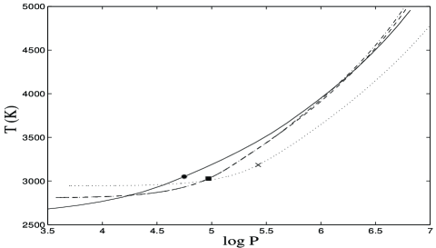
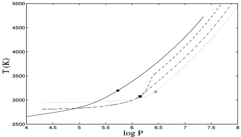
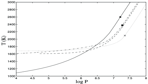
Figure 5: $P-T$ atmosphere profile according to the non-grey models of Allard & Hauschildt (1997) (solid line). Dash-dotted line: grey models obtained with the Krishna-Swamy (1966) T-$\tau$ relationship with convection included in the optically thin region. Dashed line : idem with convection arbitrarily stopped at T $\leq T_{eff}$, i.e. $\tau\sim 1$. Dotted curve : Eddington approximation. (a) $T_{eff}$ = 3500 K, $\log g=5$, [M/H]=0. The points indicate the onset of convection, corresponding to $\tau$ = 0.02 for the non-grey model (circle), $\tau$ = 0.06 for the Krishna-Swamy case (square) and $\tau$ = 0.25 for Eddington (cross). The dashed and dot-dashed curves are undistinguishable in that case. For the dashed curve, convection sets in at T = $T_{eff}$, by definition. (b) $T_{eff}$ = 3500 K, log g =5, [M/H]=-1. Convection occurs at $\tau$ = 0.06 for the non-grey model, $\tau$ = 0.08 for the Krishna-Swamy case and $\tau$ = 0.24 for Eddington. Note the departure between the dashed and dash-dotted curve when convection sets in in the optically thin region. (c) $T_{eff}$ = 2000 K, log g =5.5, [M/H]=0. In this case, the dashed curve corresponds to a model based on the Krishna-Swamy relation with grainless Rosseland opacities (D. Alexander, private communication). Convection starts well below the photosphere ($\tau>1$) and the departure between grey and non-grey models stems essentially from strong non-grey effects.

The effect of grain formation in the atmosphere on the evolution was considered in Chabrier et al. (1996), by comparing, within a grey approximation, stellar models based on the Alexander and Fergusson (1994) Rosseland opacities and on similar dust-free opacities kindly provided by Dave Alexander. Grains were found to affect the evolution only below $\sim 1800K$. This is confirmed on figure 5c where the two grey profiles, with and without grain, yield essentially the same atmospheric structure at $T_{eff}=$2000, i.e. $\sim 0.075\,M_{\odot}$. These calculations will be reconsidered once non-grey atmosphere models with grains will be available.

These calculations show convincingly that procedures based on a grey approximation and a $T(\tau)$ relation for the derivation of VLMS evolutionary models are extremely unreliable, even though they may yield, under specific thermodynamic conditions, to (fortuitous) agreement with consistent non-grey calculations. As a general result, a grey treatment yields cooler and denser atmosphere profiles below the photosphere (cf. Saumon et al. 1994; Allard and Hauschildt 1995b), and thus overestimates the effective temperature for a given mass (Chabrier et al., 1996). Therefore, they lead to erroneous mass-luminosity and mass-$T_{eff}$ relationships, as will be discussed in §4.

3 Evolutionary tracks

As mentioned in the introduction, the present study focusses on a mass-range limited to $M\leq 0.8M_{\odot}$ and will consider the brown dwarf domain only scarcely. For larger masses, the physics of VLMS remains unchanged but variations of the mixing length parameter start to be consequential and require comparison with observations (such comparisons are considered in detail in Baraffe et al. 1997). On the other hand, a substantial improvement over existing brown dwarf models (e.g. Burrows et al. 1989; 1993), requires the derivation of non-grey atmosphere models with grains. As shown by the recent analysis of Tsuji et al. (1996), silicate and iron grains can contribute significantly to the opacity in the photosphere below $\sim 2200$ K (see also Lunine et al. 1986; Alexander and Fergusson 1994), a typical effective temperature for massive brown dwarfs with solar abundances (see §3.1).

In the following sub-sections, we present the evolution of the mechanical and thermal properties of objects ranging from 0.055 to 0.6 $M_{\odot}$, over a metallicity-range [M/H]= -2 to 0. The general properties of VLMS and BDs have already been described by numerous authors (see §1). We will not redo such an analysis in detail but rather focus on selected masses to illustrate the differences arising from the new physics (EOS, nuclear rates, non-grey model atmospheres) described in the previous section. The different mechanical and thermal properties of the present models, for various metallicities, are presented in Tables 2-7.

3.1 Mechanical and thermal properties

3.1.1 Internal structure

Figure 6 displays the behaviour of the central temperature, the radius and the degeneracy parameter along the main sequence (MS) for two metallicities, [M/H]=0 (solid line) and [M/H]=-1.5 (dashed line). For stars on the MS, the internal temperature is large enough in the stellar interior for the pressure to be dominated by classical contributions ($P=\rho kT/\mu m_{H}$), so that hydrostatic equilibrium yields $R\propto M/T$. Below $\sim 0.15\,M_{\odot}$, the object is dense and cool enough for the electrons to become substantially degenerate ($\psi\propto T/\rho^{2/3}$), so that the electronic quantum contribution ($P\propto\rho^{5/3}$) overwhelms the ionic classical pressure. Eventually this will yield the well-known mass-radius relation for fully degenerate (zero-temperature) objects $R\propto M^{-1/3}$. The brown dwarf domain lies between these two limits (classical and fully degenerate) and is characterized by $R\sim R_{0}(1+\psi)$ $\sim 10^{-1}\,R_{\odot}$, about Jupiter radius, where $R_{0}$ is the zero-temperature (fully degenerate) radius (see e.g. Stevenson, 1991). The transition between the stellar and sub-stellar domains is characterized by this ongoing electron degeneracy in the interior, as illustrated in Figure 6. Note also that once degeneracy sets in, the temperature scales as $T\sim M/R-M^{2/3}/R^{2}$, where the first and second term represent the classical and quantum gas contributions, respectively. This yields the rapid drop of the interior temperature (and effective temperature for a given $T_{eff}-T_{int}$ relation) near the sub-stellar transition, and thus the characteristic severe drop in the luminosity ($L\propto R^{2}T_{eff}^{4}$).

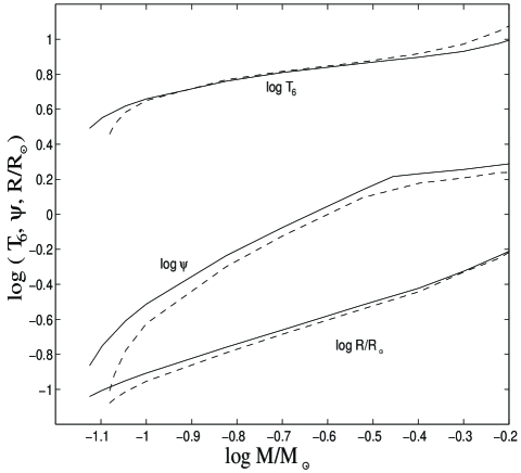
Figure 6: Degeneracy parameter $\psi=T/T_{F}$, central temperature $T_{C}$ (in units of $10^{6}$ K) and radius ($R/R_{\odot}$), as function of mass for [M/H]=0 (solid line) and [M/H]=-1.5 (dash).

Figure 7 displays the evolution of the radius for different masses. Although the radius is fixed mainly by the EOS, it does depend, to some extent, on the atmosphere treatment. The effect is negligible for solar metallicity, as shown on the figure for $m=0.2\,M_{\odot}$, but can yield $\sim 3\%$ difference on the final radius for $[M/H]=-1.5$. After a similar pre-MS contraction phase for all masses, the hydrogen-burning stars reach hydrostatic equilibrium whereas objects below the hydrogen-burning minimum mass keep contracting until reaching eventually the afore-mentioned asymptotic radius, characteristic of a strongly degenerate interior.

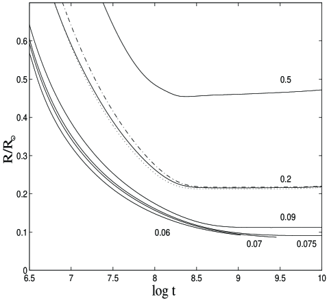
Figure 7: Evolution of the radius (in solar unit) for different masses, for solar metallicity. For 0.2 $M_{\odot}$, comparison is shown with results obtained with the Krishna-Swamy T-$\tau$ relationship (dash-dotted curve) and with the Eddington approximation (dotted line).

3.1.2 Luminosity

Figures 8a-b exhibit $L(t)$ for different masses, for $[M/H]=0$ and $[M/H]=-1.5$, respectively. Initial deuterium burning proceeds very quickly, at the very early stages of evolution, and lasts about $\sim 10^{6}-10^{7}$ years. Our calculations were done with an initial deuterium abundance $[d]_{0}=2\times 10^{-5}$ in mass fraction, which corresponds to the average abundance in the interstellar matter (cf. Linsky et al. 1993). A value $[d]_{0}=5\times 10^{-5}$ increases the deuterium burning timescale by a factor $\sim$ 2 and the luminosity by 10% to 50% during this phase. We verified that this effect is inconsequential for the rest of the evolution. As clearly shown on the figures, for masses above $0.07\,M_{\odot}$ for [M/H]=0 and $0.08\,M_{\odot}$ for [M/H]=-1.5, the internal energy provided by nuclear burning quickly balances the contraction gravitational energy, and the lowest-mass star reaches complete thermal equilibrium ($L=\int\epsilon dm$, where $\epsilon$ is the nuclear energy rate), after $\sim 1$ Gyr, for both metallicities. The lowest mass for which thermal equilibrium is reached defines the so-called hydrogen-burning minimum mass (HBMM), and the related hydrogen-burning minimum luminosity (HBML). These values are given in Tables 2-7, for various metallicities. Note the quick decrease of luminosity with time for objects below the HBMM, with $L\propto 1/t$ (cf. Burrows et al. 1989; Stevenson 1991). As mentioned above, we have not explored the BD domain and we stopped the calculations at 10 Gyrs for MS stars. Cooler models require non-grey atmospheres with grains.

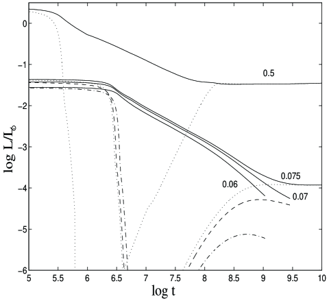
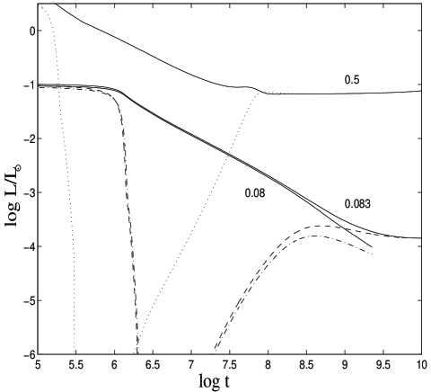
Figure 8: (a) Evolution of the luminosity for different masses for $[M/H]=0$. Solid lines: total luminosity. Nuclear luminosity $L_{nuc}$ : dotted line : 0.5 $M_{\odot}$ and 0.075 $M_{\odot}$; dashed line : $0.07M_{\odot}$; dash-dot line : $0.06M_{\odot}$. (b) Same as figure 8a for $[M/H]=-1.5.$ Nuclear luminosity $L_{nuc}$ : dotted line : 0.5 $M_{\odot}$; dashed line : $0.083M_{\odot}$; dash-dot line : $0.08M_{\odot}$.

As already shown by Chabrier et al. (1996), stellar models based on non-grey model atmospheres yield smaller HBMM than grey models, a direct consequence of the lower effective temperature and luminosity, as discussed in the previous section. The larger the luminosity, for a given mass, the larger the required central temperature to reach thermal equilibrium, which in turns implies a larger contraction (density) and degeneracy.

As illustrated on Fig. 8, slightly below $\sim 0.072\,M_{\odot}$ (resp. 0.083 $M_{\odot}$) for [M/H]=0 (resp. [M/H] $\leq$ -1), nuclear ignition still takes place in the central part of the star, but cannot balance steadily the ongoing gravitational contraction. This defines the massive brown dwarfs. The evolution equation thus reads $L=\int\epsilon dm\,\,-\,\,\int T{dS\over dt}dm$, where the second term on the right hand side of the equation stems from the contraction energy plus the internal energy released along evolution. As shown in Fig. 7, contraction is fairly small after $\sim 10^{8}$ yr, so that most of the luminosity arises from the thermal content. Below about $0.07\,M_{\odot}$ (resp. $0.08\,M_{\odot}$) for [M/H]=0 (resp. [M/H] $\leq$ -0.5), the energetic contribution arising from hydrogen-burning, though still present for the most massive objects, is order of magnitudes smaller than the internal energy, which provides essentially all the energy of the star ($\epsilon<<T|{dS\over dt}|$).

As seen in the figures, objects with lower metallicity evolve at larger luminosities and effective temperatures, a well-known result. The effects of metallicity on the atmosphere structure have been discussed extensively by Brett (1995) and AH95 but can be apprehended with intuitive arguments. The lower the metallicity, the lower the opacity and the more transparent the atmosphere. The same optical depth thus lies at deeper levels, i.e. at higher pressure (${dP\over d\tau}={g\over\kappa}$). Therefore, for a given mass ($\log g$), the $(T,P)$ interior profile matches, for a given optical depth $\tau$, an atmosphere profile with larger $T_{eff}$ (see Fig. 5). This yields a larger luminosity, since the radius barely depends on the atmosphere, as shown previously.

Objects above 0.15 $M_{\odot}$ reach the MS in $t_{MS}\mathrel{\hbox{\hbox to0.0pt{\lower 2.15277pt\hbox{$\sim$}\hss}\raise 1.72218pt\hbox{$<$}}}3\times 10^{8}$ yrs, while it takes $3\times 10^{8}<t_{MS}<2.5\times 10^{9}$ yrs (resp. $t_{MS}\mathrel{\hbox{\hbox to0.0pt{\lower 2.15277pt\hbox{$\sim$}\hss}\raise 1.72218pt\hbox{$<$}}}2\times 10^{9}$ yrs) for $[M/H]=0$ (resp. $[M/H]\leq-1.0$) for objects in the range $0.075<M/M_{\odot}<0.15$. Objects above $M\sim 0.9M_{\odot}$ (resp. $M\sim 0.8M_{\odot}$) for $[M/H]=0$ (resp. $[M/H]\leq-1$) start evolving off the MS at $t=10$ Gyr.

As shown on Figure 8, an object on the pre-MS contraction phase which will eventually become a H-burning star ($M\mathrel{\hbox{\hbox to0.0pt{\lower 2.15277pt\hbox{$\sim$}\hss}\raise 1.72218pt\hbox{$>$}}}0.075\,M_{\odot}$) can have the same luminosity and effective temperature as a bona-fide brown dwarf.

3.2 Full convection limit

Solar-like stars are essentially radiative, except for a small convective region in the outermost part of the envelope, due to hydrogen partial ionisation, and sometimes for a small convective core where nuclear burning takes place. As the mass decreases, the internal temperature decreases ($T\propto M$), the inner radiative region shrinks and vanishes eventually for a certain mass below which the star becomes entirely convective (see e.g. D’Antona & Mazzitelli 1985, Dorman et al. 1989). This transition mass $M_{conv}$ has been determined with grey atmosphere models, which become invalid below $\sim 5000$ K, and thus must be recalculated accurately. Figure 9 shows the interior structure of stars with $M\geq 0.4M_{\odot}$ as a function of time for [M/H]=0. The pre-MS contraction phase proceeds at constant $T/\rho^{1/3}$, i.e. constant $R_{OPAL}$ ( $R_{OPAL}=\log\rho/T_{6}^{3}$). After $\sim 10^{7}$ years, a radiative core develops and grows. The physical reason is the decreasing opacity after the last bump due to metal absorption (mainly $Fe$,), for $T_{6}\mathrel{\hbox{\hbox to0.0pt{\lower 2.15277pt\hbox{$\sim$}\hss}\raise 1.72218pt\hbox{$>$}}}2-3$ (this temperature decreases with metallicity) (cf. Rogers and Iglesias 1992, Fig. 2). The radiative core thus appears earlier for the more massive, hotter, stars. The minimum mass for the onset of radiation in the core is found to be $M_{conv}=0.35\,M_{\odot}$, for all the studied metallicites ($-2\leq[M/H]\leq 0)$. After $\sim 10^{8}$ years, the star reaches thermal equilibrium, nuclear fusion proceeds at the center, and a small convective core develops for a certain time, depending on the mass and the metallicity, bracketting the central radiative region between two convective zones. We verified that the growth of the central convective core is governed by the ${}^{3}He+^{3}He$ reaction. The nuclear energy released by the $p+p$ and $p+d$ reactions is insufficient to generate convective instability. As long as the reaction given by eqn.(2) dominates, the ${}^{3}He$ abundance, and thus the convective core, increases. The situation reverses as soon as the central temperature is high enough for ${}^{3}He$ to reach its equilibrium abundance (eqns. (2)+(3)), wich decreases with increasing temperature (see e.g. Clayton 1968, Fig. 5.4).

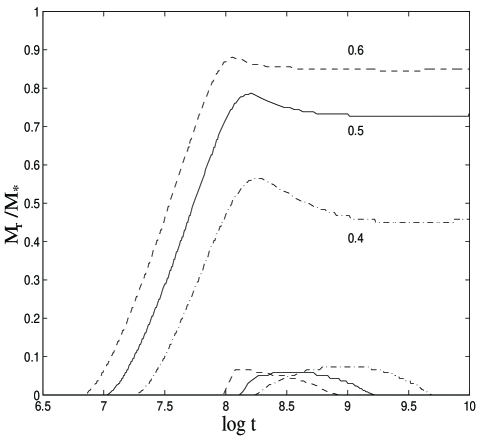
Figure 9: Evolution of the radiative zone $M_{rad}/M_{\star}$ for [M/H]=0. The upper curves determine the bottom of the convective enveloppe and the lower curves the top of the convective core for 0.4 $M_{\odot}$ (dash-dot), 0.5 $M_{\odot}$ (solid line) and 0.6 $M_{\odot}$ (dash).

The extension of the afore-mentioned radiative region decreases with temperature, and thus with mass, as shown on the figure. For the afore-mentioned limit-mass $0.35\,M_{\odot}$, this inner radiative zone remains only for $[M/H]=-1.0$. For all other (greater and smaller) metallicities, it vanishes as soon as the convective core appears. In this case the 0.35 $M_{\odot}$ star will become fully convective again after $\sim 3\,10^{9}$ yrs. This rather complicated dependence on metallicity stems from the subtle competiton between the decreasing opacity, which favors radiation, and the increasing pressure and luminosity which inhibate radiation and favor convection, with decreasing metallicity ($\nabla_{rad}\propto{L\kappa P\over T^{4}}$). This yields the minimum value for $M_{conv}$ for $[M/H]=-1$.

Table 1 gives the position of the bottom of the convective enveloppe as a function of mass and metallicity. We also give the results for the masses of the binary system YY-Gem. Note that grey models, which have higher luminosity (see §4.1), thus have a larger $\nabla_{rad}$, which favors convection and thus yields larger convective envelopes and larger convective cores and $M_{conv}$. As will be shown below, the onset of a radiative core, and the retraction of the bottom of the convective zone to outer, cooler regions bears important consequences on the abundance of light elements in the envelope.

3.3 Abundance of light elements

Observation of lithium in the atmosphere of VLMS is a powerful diagnostic for the identification of genuine brown dwarfs, as proposed initially by Rebolo and collaborators (Rebolo, Martin & Magazzù 1992). The first theoretical analysis of light-element burning in VLMS, and the expected abundances along evolution, were carried by Pozio (1991) and Nelson, Rappaport and Chiang (1993). As for the convective limit, this analysis must be redone with updated EOS, screening factors and atmosphere models. The initial abundances were taken to be $[^{7}Li]_{0}=10^{-9}$, $[^{9}Be]_{0}=10^{-10}$ and $[^{11}B]_{0}=3\times 10^{-11}$, as in Nelson et al. (1993). The modification of the abundances along evolution, i.e. the depletion factor, is given by $X_{i}/X_{i_{0}}$, where $X_{i}$ is the abundance of element $i$ at a given time and $X_{i_{0}}$ is the afore-mentioned initial abundance. The burning temperatures for these elements (in the vacuum) are $T_{Li}\sim 2\times 10^{6}$ K, $T_{Be}\sim 3\times 10^{6}$ K and $T_{B}\sim 4\times 10^{6}$ K, respectively.

As for hydrogen, burning ignition temperatures translate into minimum burning masses. Using the ion+electron screening factors mentioned in §2.2, we get the following values, for solar metallicity : $M_{Li}/M_{\odot}=\,0.055$, $M_{Be}/M_{\odot}=\,0.065$ and $M_{B}/M_{\odot}=0.08$. For comparison, Nelson et al. (1993) find that $\sim\,50\%$ of ⁷Li is burned in a 0.059 $M_{\odot}$, whereas this value is already reached in our 0.055 $M_{\odot}$ model. D’Antona & Mazzitelli (1994) obtain $M_{Li}/M_{\odot}=\,0.065$. This less efficient nuclear burning in Nelson et al. and DM94 stems on one hand from the grey approximation, which yields larger $L$ and $T_{eff}$ and thus central densities, which favors the onset of degeneracy (cf. §3.1.2 and Fig. 10 below), and also from the smaller Graboske et al. (1973) screening factors (see Figure 3).

These effects, and the metallicity dependence, are illustrated in Figures 10a-b which display the evolution of central temperature and lithium-abundance, respectively, for different metallicities. Comparison is made with a solar metallicity model of DM94 (cf. their Table 7). The denser metal poor stars (and grey models) reach the limit of degeneracy ealier ($\psi\propto\rho^{-2/3}$), yielding a lower maximum central temperature for metal poor objects. The direct consequence is an increasing minimum burning mass with decreasing metallicity, $M_{Li}/M_{\odot}=\,0.06$ for [M/H] $\leq-1$ instead of $0.055$ for [M/H] $\sim 0$.

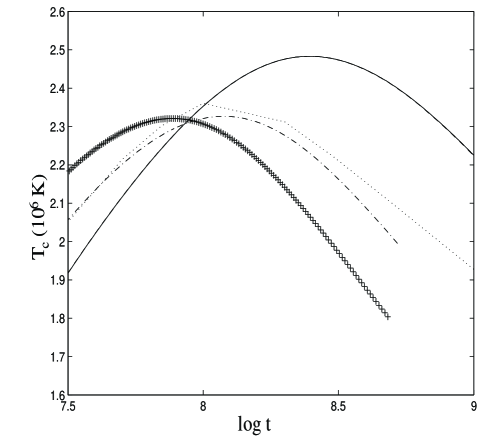
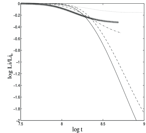
Figure 10: (a) Evolution of the central temperature in a 0.06 $M_{\odot}$ brown dwarf. Solid line : $[M/H]=0$; dot-dash line : $[M/H]=-1.0$; ($+$) : $[M/H]=-2.0$. Dotted line: 0.06 $M_{\odot}$ of DM94 for [M/H]=0. Dashed line : calculations with the Graboske et al. (1973) screening factors, for $[M/H]=0$. Note that the solid and dashed curves are undistinguishable, and illustrate the negligible effect of the electronic screening factor on the evolution of LMS. (b) Same as figure 10a for the abundance of Lithium w.r.t. its initial abundance. Same legends as in figure 10a.

Figure 11 shows the abundances of $Li$, $Be$ and $B$ as a function of mass and metallicity. The gaps correspond to fully convective interiors, as described in §3.2. In that case, convective mixing brings the elements present in the envelope down to the central burning region where they are destroyed. Above 0.4 $M_{\odot}$, the central radiative core appears and the bottom of the convection zone retracts to cooler regions, as described previously. As mentioned above, this depends mainly on the central opacity : the larger the opacity, and thus the metal-abundance, the larger the central temperature required to allow radiative transport ($\nabla_{rad}\propto\kappa/T^{4}$). This yields more efficient depletion with increasing metallicity, as illustrated on the figure. Lithium is totally destroyed in the mass range 0.075-0.6 $M_{\odot}$ for [M/H]=0, whereas it reappears for M $\mathrel{\hbox{\hbox to0.0pt{\lower 2.15277pt\hbox{$\sim$}\hss}\raise 1.72218pt\hbox{$>$}}}0.5M_{\odot}$ for [M/H] $\leq$ -1. However, below [M/H]=-1.5, the situation seems to reverse, as the [M/H]=-2 case shows a slightly higher level of depletion. At such low metallicities, the dependence of the opacity on the metallicity for T${}_{c}\geq 3\times 10^{6}K$ decreases rapidly and the dominant effect is now the higher luminosity at [M/H]=-2, which implies a larger central temperature to favor radiation ($\nabla_{rad}\propto L/T^{4}$). The depletion factors in the stellar interiors are given in Tables 2-7. The lithium depletion factors in the brown dwarf regime are given in Chabrier et al. (1996). A complete description of light elements depletion in this regime, which implies evolutionary models based on dusty atmosphere models, is under progress.

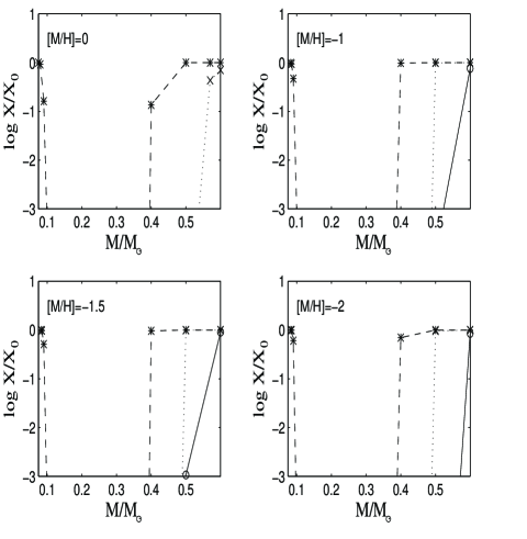
Figure 11: Abundances of light elements as a function of mass and metallicity at $t=$10 Gyrs. Only results in stars are shown ( $M\geq 0.075M_{\odot}$ for [M/H]=0 and $M\geq 0.083M_{\odot}$ for [M/H] $\leq$ -1). Abundances normalized to their initial value are shown for Li (solid,$O$), Be (dot,$X$) and B(dash, $\star$).

4 Mass-dependence of the photospheric quantities

4.1 Mass-luminosity relationship

Figure 12 shows the mass-luminosity (ML) relationship for VLMS for three metallicities, $Z=Z_{\odot}$, $Z=10^{-1.5}\times Z_{\odot}$ and $Z=0$, for $t=$10 Gyrs. The zero-metal case sets the upper limit for the luminosity for a given mass.

We first note the well-known wavy behaviour of the ML relation (see e.g. DM94). The change of slope below $M\sim 0.4-0.5\,M_{\odot}$ is due to the formation of H₂ molecules in the atmosphere (Auman 1969; Kroupa, Tout & Gilmore, 1990), which occurs at higher $T_{eff}$ for decreasing metallicity, because of the denser atmosphere (see SCVH). The steepening of the ML relation near the lower-mass end reflects the onset of ongoing degeneracy in the stellar interior, as demonstrated in §3.1.1. The previous stellar models of BCAH95, based on the $Base$ AH95 atmosphere models, are shown for comparison. We note that for solar-metallicity, the substantial improvement in the most recent atmosphere models translate into significant differences ($\sim 15\%-25\%$ in $L$ and $\sim 200$ K in $T_{eff}$), the Straight-Mean approximation used in the $Base$ models leading to an overall overestimated opacity. This difference between the models vanishes for lower metallicities (see Allard et al., 1997b). Note that the present models have been shown to reproduce accurately the mass-$M_{V}$ and mass-$M_{K}$ relationship determined observationaly by Henry & Mc Carthy (1993) down to the bottom of the MS (Chabrier et al., 1996; Allard et al., 1997a). The $ML$ relations for different metallicities are given in Tables 2-7. The comparison with other models/approximations is devoted to the next subsection.

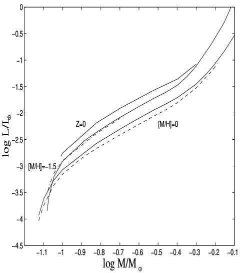
Figure 12: Mass-luminosity relationship for [M/H]=0, $[M/H]=$-1.5 and the zero-metal case Z=0. The previous results of Baraffe et al. (1995) based on the $Base$ atmosphere models are also shown ( dashed curve for [M/H]=0 and dash-dotted curve for [M/H]=-1.5).

4.2 Mass-effective temperature relationship

Figures 13 display the mass-effective temperature relationships for sub-solar (Fig. 13a) and solar (Fig. 13b) metallicities. A shown in Fig. 13a, our zero-metal models reproduce correctly the models of Saumon et al. (1994)(filled circles). Figures 13 also display the $m-T_{eff}$ relation obtained with the Krishna-Swamy $T(\tau)$ relationship, with (dotted line) and without (dot-dashed line) convection in the optically thin region (cf. §2.5). The figures clearly show the overestimated effective temperature obtained by grey models using a diffusion approximation (Burrows et al. 1989, ($+$); DM94 (squares); DM96 (triangles)), as demonstrated in §2.5.

As already mentioned, the Krishna-Swamy relationship with convection arbitrarily suppressed at $\tau<1$ (Alexander et al. 1996, ($X$)) leads to less severe discrepancy in the region where convection does penetrate into the optically thin layers (2500 K $<T_{eff}<$ 5000 K). This paradoxal and inconsistent situation clearly illustrates the dubious reliability of such a treatment, and reflects the unreliable representation of the effects of atmospheric convection within a grey-approximation. This is clearly illustrated by the rather unphysical atmospheric profile obtained within this approximation, as shown in Figure 5b. For solar metallicity, however, both KS grey approximations yield a similarly good match to the innermost part of the atmosphere profile (see §2.5). It is the reason why the KS treatment with convection in the optically thin region, as used in Dorman et al. (1989) (filled circles), yields a reasonable agreement at solar metallicity, whereas it yields severe discrepancies for lower metallicities. This reflects the significant overestimation of the convective flux as density and pressure increase with decreasing metallicity. Models based on the Eddington approximation predict even higher $T_{eff}$ at a given mass (see Fig. 5).

The unreliability of any $T(\tau)$ relationship for VLMS becomes even more severe near the bottom of the MS ( $m<0.1M_{\odot}$), as shown on the figures. They yield too steep $m-T_{eff}$ relationships in the stellar-to-substellar transition region and thus too large HBMMs, by $\sim 10\%$, as discussed in §3.1.2. The difference between grey and non-grey calculations vanishes for $T_{eff}\mathrel{\hbox{\hbox to0.0pt{\lower 2.15277pt\hbox{$\sim$}\hss}\raise 1.72218pt\hbox{$>$}}}6000$ K, i.e. $\sim 0.8\,M_{\odot}$ for metal-depleted abundances. For a 0.8 $M_{\odot}$ star with $[M/H]<0$, the difference between models based on non-grey AH97 atmospheres and on grey models calculated with Alexander and Fergusson (1994) Rosseland opacities amounts to $\sim$ 1-2% in $T_{eff}$ and less than 1% in L.

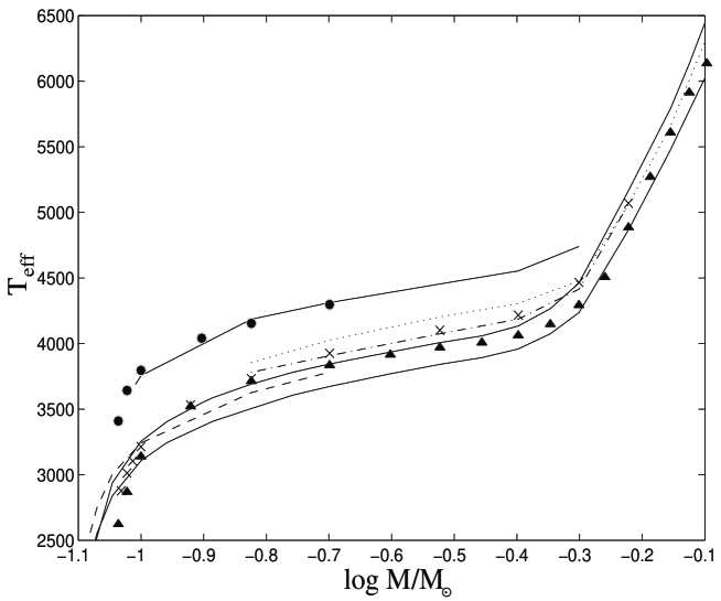
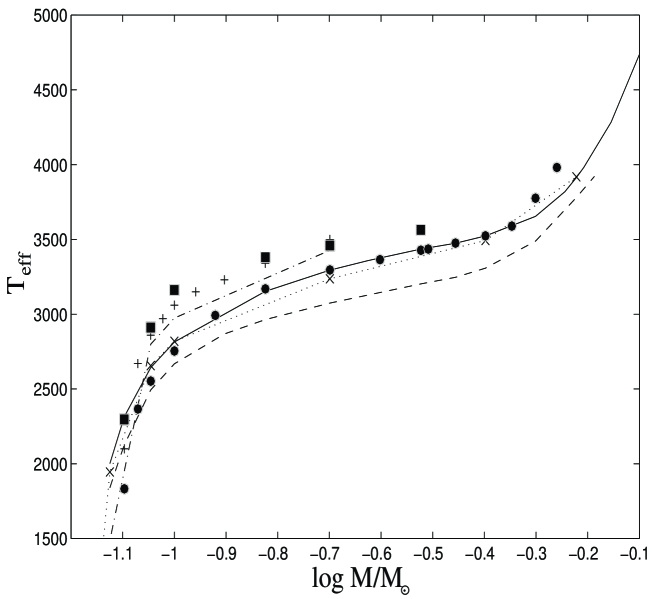
Figure 13: (a) Mass-effective temperature relationship for low-metallicity. Solid lines : present models for $Z=0$ and $[M/H]=-1.5,\,-1.0$, from top to bottom. Dashed line : non-grey models based on the $Base$ atmosphere models for $[M/H]=-1.5$ (BCAH95). Dotted line and dot-dashed line : models for [M/H]=-1.5 based on the Krishna-Swamy $T(\tau)$ relationship with (dot) and without (dash-dot) convection in the optically thin region. Crosses : the [M/H]=-1.5 models of Alexander et al. (1996). Triangles : the [M/H]=-1.0 models of D’Antona and Mazzitelli (1996). Full circles : the Z=0 models of Saumon et al. (1994). (b) Same as figure 13a for solar metallicity. Solid and dashed lines as in Fig. 13a. Dash-dotted line : Eddington approximation. Dotted line (and crosses) : Krishna-Swamy relationship. Comparison with previous works: Burrows et al. (1989), models G ($+$); D’Antona & Mazzitelli (1994), models with the Alexander opacities and the MLT (full squares); Dorman et al. (1989), models with the FGV EOS (full circles).

The different mass-$T_{eff}$ relations are given in Tables 2-7. Differences between effective temperatures as a function of the metallicity, for a given mass, $(\Delta T_{eff}/\Delta Z)_{M}$, decrease with mass. The 0.5 $M_{\odot}$ star with [M/H]=-1.5 is $\sim$ 800 K hotter than its solar metallicity counterpart, whereas the difference reduces to $\sim 300K$ for the 0.09 $M_{\odot}$. This stems from the decreasing sensitivity of the atmosphere structure to metal abundance with decreasing $T_{eff}$ (see e.g. Allard, 1990; Brett, 1995; AH97).

5 Conclusion

In this paper, we have presented new calculations aimed at describing the structure and the evolution of low mass stars, from solar masses down to the hydrogen burning limit, for a wide range of metallicities. These calculations include the most recent physics aimed at describing the mechanical and thermal properties of these objects - equation of state, screening factors for the nuclear reaction rates, non-grey atmosphere models -. The Saumon-Chabrier hydrogen-helium EOS gives the most accurate description of the internal properties of these objects over the entire afore-mentioned mass range. Given their negligible number abundance, metals play essentially no role on the EOS itself and their presence is mimicked adequately by an effective helium fraction. Of course they do play a role as electron donors for the opacities and must be included in the appropriate ionization equilibrium equations when opacities are concerned. Note that, for the densest stars ($0.1\,M_{\odot}$, $[M/H]=-2.0$, $\log g=5.5$), departure from ideality at $\tau=100$ (resp. $\tau=1$) in the atmosphere is found to represent $\sim 3\%$ (resp. $\sim 1\%$) on the adiabatic gradient (as obtained from a comparison between the complete SC EOS vs an ideal gas EOS). Thus, under LMS conditions, an ideal (Saha) EOS can be safely used over the entire atmosphere, for metallicities $[M/H]\geq-2$. Note that an (incorrect) grey approximation yield denser atmospheric profiles (cf §2.4) and thus will overestimate non-ideal effects.

We show that under LMS conditions, the responsive electron background participates to the screening of the nuclear reactions, and must be included for an accurate determination of the various minimum burning masses and of the abundances of light elements along evolution. We show that, near the bottom of the main sequence, the deuterium lifetime against proton capture in the PPI chain is order of magnitudes smaller than the convective mixing time. Instantaneous mixing is thus no longer satisfied. This yields the presence of a deuterium gradient in the burning core, which bears substantial consequences on the determination of the luminosity near the brown dwarf regime.

We have examined carefully the effect of various grey-like approximations on the evolution and the mass-calibration of LMS. Under LMS conditions, these prescriptions are incorrect, or at best unreliable, and yield inaccurate mass-luminosity and mass-effective temperature relationships, which in turn yield inaccurate mass functions from observed luminosity functions. We examine the behaviour of the different stellar macroscopic quantities, radius, temperature, luminosity, as functions of mass, time and metallicity. We link the general behaviour of these quantities to intrinsic physical properties of stellar matter, in particular the transition from classical to quantum objects and the onset of convection or radiation in the stellar interior and atmosphere. We derive new limits for the hydrogen-burning minimum mass, effective temperature and luminosity, for each metallicity. These limits are smaller than the values determined previously, a direct consequence of non-grey effects in the atmosphere.

We believe the present calculations to represent a significant improvement in low-mass star theory and in our understanding of the properties of cool and dense objects. This provides solid grounds to examine the structure and the evolution of substellar objects, brown dwarfs and exoplanets.

At last the present models provide reliable mass-luminosity relationships, a cornerstone for the derivation of accurate mass functions (Méra, Chabrier & Baraffe, 1996; Chabrier & Méra, 1997). The comparison with observations has already been presented in different Letters (see references), and is examined in detail in two companion papers, namely Baraffe et al. (1997) for metal-poor globular cluster and halo field stars and in Allard et al. (1997a) for solar-like abundances.

Tables 2-7 are available by anonymous ftp:

ftp ftp.ens-lyon.fr

username: anonymous

ftp $>$ cd /pub/users/CRAL/ibaraffe

ftp $>$ get CB97_models

ftp $>$ quit

Table 1: Bottom of the convective enveloppe $R_{CE}$ normalised to the radius of the star R as a function of mass and metallicity, for an age of 10 Gyrs. Comparison is made with grey models based on the Krishna-Swamy prescription for the 0.4 $M_{\odot}$ and [M/H]=-1.5. The values 0.57 and 0.62 $M_{\odot}$ correspond to the eclipsing binary system YY-Gem (Leung and Schneider 1978)

[M/H]	$M/M_{\odot}$	${\rm log}L/L_{\odot}$	R ($10^{10}$ cm)	$R_{CE}$/R
0	0.4	-1.71	2.640	0.49
	0.5	-1.45	3.285	0.61
	0.57	-1.25	3.806	0.64
	0.6	-1.15	4.035	0.65
	0.62	-1.09	4.189	0.66
-1	0.35	-1.66	2.269	0.43
	0.40	-1.53	2.566	0.58
	0.50	-1.18	3.335	0.69
	0.60	-0.782	4.013	0.73
-1.5	0.4	-1.47	2.517	0.58
	0.5	-1.12	3.252	0.69
	0.60	-0.70	3.904	0.75
-1.5 $Grey$	0.4	-1.42	2.455	0.54
-2	0.4	-1.42	2.460	0.55
	0.5	-1.08	3.148	0.69
	0.60	-0.67	3.837	0.76

Table 2: Properties of Very Low mass stars for [M/H]=0 and Y=0.275. Central temperature $T_{c}$ is in K and density $\rho_{c}$ in $gr\,cm^{-3}$. Abundances of light elements are normalised to their initial abundance (see text).

$M/M_{\odot}$	age (Gyrs)	$T_{eff}$	log $L/L_{\odot}$	R ($10^{10}$ cm)	log $T_{c}$	log $\rho_{c}$	Li/Li0	Be/Be0	B/B0
0.075	0.01	3006.	-2.048	2.449	6.199	1.108	1.00000	1.00000	1.00000
	0.10	2835.	-2.831	1.118	6.459	2.125	0.35600	0.99800	1.00000
	1.00	2211.	-3.695	0.680	6.510	2.789	0.00000	0.03180	1.00000
	10.00	2002.	-3.929	0.634	6.492	2.882	0.00000	0.00000	0.99667
0.080	0.01	3025.	-2.010	2.528	6.215	1.097	1.00000	1.00000	1.00000
	0.10	2876.	-2.780	1.152	6.482	2.117	0.17100	0.99400	1.00000
	1.00	2374.	-3.536	0.708	6.554	2.765	0.00000	0.00120	0.99333
	10.00	2314.	-3.605	0.689	6.552	2.803	0.00000	0.00000	0.91667
0.090	0.01	3059.	-1.939	2.682	6.242	1.076	1.00000	1.00000	1.00000
	0.10	2946.	-2.694	1.213	6.522	2.106	0.02050	0.96100	1.00000
	1.00	2645.	-3.261	0.784	6.617	2.686	0.00000	0.00000	0.90333
	10.00	2642.	-3.265	0.781	6.619	2.691	0.00000	0.00000	0.16200
0.100	0.01	3090.	-1.874	2.833	6.266	1.054	1.00000	1.00000	1.00000
	0.10	3006.	-2.614	1.278	6.555	2.087	0.00180	0.85200	1.00000
	1.00	2811.	-3.070	0.863	6.658	2.607	0.00000	0.00000	0.59333
	10.00	2814.	-3.069	0.863	6.659	2.607	0.00000	0.00000	0.00038
0.110	0.01	3112.	-1.821	2.968	6.288	1.038	1.00000	1.00000	1.00000
	0.10	3051.	-2.550	1.334	6.585	2.075	0.00009	0.61000	1.00000
	1.00	2919.	-2.932	0.939	6.687	2.539	0.00000	0.00000	0.26533
	10.00	2922.	-2.929	0.940	6.688	2.538	0.00000	0.00000	0.00000
0.150	0.01	3186.	-1.636	3.503	6.354	0.964	1.00000	1.00000	1.00000
	0.10	3199.	-2.328	1.567	6.669	2.009	0.00000	0.02640	0.99667
	1.00	3149.	-2.581	1.209	6.759	2.349	0.00000	0.00000	0.00293
	10.00	3153.	-2.577	1.212	6.760	2.346	0.00000	0.00000	0.00000
0.200	0.01	3251.	-1.464	4.101	6.412	0.889	1.00000	1.00000	1.00000
	0.10	3299.	-2.137	1.835	6.738	1.934	0.00000	0.00009	0.91000
	1.00	3290.	-2.316	1.502	6.813	2.196	0.00000	0.00000	0.00000
	10.00	3295.	-2.302	1.523	6.810	2.177	0.00000	0.00000	0.00000
0.300	0.01	3345.	-1.232	5.060	6.498	0.798	0.98700	1.00000	1.00000
	0.10	3424.	-1.873	2.310	6.818	1.831	0.00000	0.00000	0.79333
	1.00	3437.	-1.984	2.016	6.879	1.996	0.00000	0.00000	0.00000
	10.00	3436.	-1.945	2.112	6.863	1.935	0.00000	0.00000	0.00000
0.350	0.01	3396.	-1.138	5.469	6.531	0.766	0.95300	1.00000	1.00000
	0.10	3471.	-1.767	2.540	6.836	1.821	0.00000	0.00000	0.97667
	1.00	3478.	-1.857	2.282	6.897	1.907	0.00000	0.00000	0.00847
	10.00	3475.	-1.822	2.380	6.882	1.850	0.00000	0.00000	0.00000
0.400	0.01	3451.	-1.050	5.863	6.559	0.735	0.87600	1.00000	1.00000
	0.10	3525.	-1.660	2.786	6.853	1.827	0.00000	0.00016	0.99667
	1.00	3522.	-1.727	2.581	6.905	1.852	0.00000	0.00000	0.82667
	10.00	3524.	-1.707	2.640	6.897	1.859	0.00000	0.00000	0.13533
0.500	0.01	3555.	-0.903	6.547	6.608	0.691	0.52200	0.99700	1.00000
	0.10	3658.	-1.429	3.374	6.898	1.875	0.00000	0.30000	1.00000
	1.00	3649.	-1.478	3.205	6.935	1.848	0.00000	0.09220	1.00000
	10.00	3654.	-1.454	3.285	6.930	1.880	0.00000	0.00000	1.00000
0.600	0.01	3645.	-0.785	7.134	6.645	0.668	0.28900	0.99300	1.00000
	0.10	3987.	-1.119	4.058	6.979	1.935	0.00000	0.86400	1.00000
	1.00	3883.	-1.195	3.919	6.969	1.860	0.00000	0.84200	1.00000
	10.00	3914.	-1.156	4.035	6.976	1.921	0.00000	0.70200	1.00000
0.700	0.01	3719.	-0.681	7.721	6.669	0.655	0.38200	0.99600	1.00000
	0.10	4246.	-0.910	4.551	7.027	1.880	0.00205	0.97400	1.00000
	1.00	4209.	-0.909	4.637	7.009	1.876	0.00105	0.97300	1.00000
	10.00	4284.	-0.841	4.841	7.031	1.992	0.00000	0.96800	1.00000
0.800	0.01	4091.	-0.539	7.515	6.729	0.796	0.10400	0.98900	1.00000
	0.10	4647.	-0.647	5.140	7.059	1.876	0.00173	0.97000	1.00000
	1.00	4647.	-0.632	5.235	7.051	1.897	0.00157	0.97000	1.00000
	10.00	4762.	-0.515	5.705	7.097	2.111	0.00085	0.96900	1.00000

Table 3: Same as Table 2 for [M/H]=-0.5 and Y=0.25

$M/M_{\odot}$	age (Gyrs)	$T_{eff}$	log $L/L_{\odot}$	R ($10^{10}$ cm)	log $T_{c}$	log $\rho_{c}$	Li/Li0	Be/Be0	B/B0
0.080	0.01	3211.	-1.988	2.299	6.238	1.218	1.00000	1.00000	1.00000
	0.10	3023.	-2.759	1.068	6.483	2.215	0.09320	0.99000	1.00000
	1.00	2352.	-3.608	0.664	6.508	2.849	0.00000	0.00772	1.00000
	10.00	2128.	-3.835	0.625	6.485	2.928	0.00000	0.00000	0.99333
0.090	0.01	3246.	-1.918	2.441	6.266	1.196	1.00000	1.00000	1.00000
	0.10	3102.	-2.666	1.129	6.525	2.198	0.00708	0.93400	1.00000
	1.00	2725.	-3.261	0.738	6.594	2.764	0.00000	0.00000	0.95333
	10.00	2716.	-3.271	0.734	6.595	2.772	0.00000	0.00000	0.45333
0.100	0.01	3279.	-1.852	2.580	6.290	1.173	1.00000	1.00000	1.00000
	0.10	3160.	-2.593	1.184	6.562	2.186	0.00026	0.73100	1.00000
	1.00	2940.	-3.035	0.822	6.644	2.671	0.00000	0.00000	0.67000
	10.00	2943.	-3.033	0.823	6.646	2.670	0.00000	0.00000	0.00282
0.110	0.01	3309.	-1.797	2.700	6.313	1.158	1.00000	1.00000	1.00000
	0.10	3211.	-2.522	1.244	6.591	2.167	0.00001	0.44300	1.00000
	1.00	3068.	-2.882	0.900	6.677	2.595	0.00000	0.00000	0.29133
	10.00	3072.	-2.879	0.901	6.679	2.593	0.00000	0.00000	0.00000
0.150	0.01	3399.	-1.606	3.187	6.380	1.085	1.00000	1.00000	1.00000
	0.10	3353.	-2.310	1.457	6.681	2.103	0.00000	0.00543	0.99000
	1.00	3311.	-2.521	1.172	6.754	2.390	0.00000	0.00000	0.00320
	10.00	3314.	-2.517	1.175	6.756	2.386	0.00000	0.00000	0.00000
0.200	0.01	3479.	-1.435	3.704	6.442	1.020	0.99800	1.00000	1.00000
	0.10	3467.	-2.115	1.705	6.752	2.030	0.00000	0.00000	0.77333
	1.00	3451.	-2.257	1.462	6.809	2.230	0.00000	0.00000	0.00000
	10.00	3455.	-2.241	1.485	6.806	2.211	0.00000	0.00000	0.00000
0.300	0.01	3595.	-1.193	4.586	6.526	0.924	0.94000	1.00000	1.00000
	0.10	3640.	-1.827	2.154	6.831	1.928	0.00000	0.00000	0.90000
	1.00	3640.	-1.909	1.960	6.877	2.032	0.00000	0.00000	0.00000
	10.00	3645.	-1.865	2.058	6.860	1.969	0.00000	0.00000	0.00000
0.350	0.01	3648.	-1.100	4.956	6.560	0.892	0.81000	0.99900	1.00000
	0.10	3703.	-1.708	2.389	6.850	1.928	0.00000	0.00027	0.99667
	1.00	3696.	-1.759	2.260	6.888	1.923	0.00000	0.00000	0.19033
	10.00	3697.	-1.742	2.305	6.883	1.895	0.00000	0.00000	0.00000
0.400	0.01	3702.	-1.016	5.298	6.589	0.865	0.58500	0.99800	1.00000
	0.10	3777.	-1.582	2.656	6.874	1.947	0.00000	0.16200	1.00000
	1.00	3754.	-1.630	2.541	6.903	1.905	0.00000	0.00027	0.99000
	10.00	3759.	-1.609	2.598	6.899	1.919	0.00000	0.00000	0.94667
0.500	0.01	3810.	-0.875	5.887	6.633	0.841	0.44400	0.99700	1.00000
	0.10	4033.	-1.269	3.338	6.950	1.997	0.00011	0.95900	1.00000
	1.00	3947.	-1.333	3.237	6.941	1.901	0.00000	0.93700	1.00000
	10.00	3968.	-1.298	3.333	6.944	1.954	0.00000	0.84900	1.00000
0.600	0.01	3920.	-0.748	6.433	6.662	0.847	0.67000	0.99900	1.00000
	0.10	4357.	-1.008	3.862	7.002	1.941	0.25400	0.99700	1.00000
	1.00	4321.	-1.000	3.960	6.986	1.914	0.22000	0.99700	1.00000
	10.00	4406.	-0.935	4.109	7.004	2.020	0.11200	0.99600	1.00000
0.700	0.01	4039.	-0.624	6.990	6.688	0.871	0.86300	1.00000	1.00000
	0.10	4804.	-0.704	4.509	7.038	1.921	0.77100	1.00000	1.00000
	1.00	4806.	-0.687	4.593	7.032	1.929	0.76500	1.00000	1.00000
	10.00	4962.	-0.569	4.933	7.075	2.136	0.74600	1.00000	1.00000
0.800	0.01	4176.	-0.498	7.560	6.715	0.916	0.95300	1.00000	1.00000
	0.10	5217.	-0.432	5.228	7.075	1.923	0.94200	1.00000	1.00000
	1.00	5225.	-0.412	5.334	7.076	1.941	0.94100	1.00000	1.00000
	10.00	5490.	-0.190	6.239	7.164	2.359	0.94100	1.00000	1.00000

Table 4: Same as Table 2 for [M/H]=-1 and Y=0.25

$M/M_{\odot}$	age (Gyrs)	$T_{eff}$	log $L/L_{\odot}$	R ($10^{10}$ cm)	log $T_{c}$	log $\rho_{c}$	Li/Li0	Be/Be0	B/B0
0.083	0.01	3421.	-1.946	2.128	6.282	1.337	1.00000	1.00000	1.00000
	0.10	3203.	-2.705	1.013	6.511	2.303	0.00747	0.94700	1.00000
	1.00	2527.	-3.504	0.649	6.521	2.897	0.00000	0.00054	0.99667
	10.00	2359.	-3.660	0.622	6.504	2.952	0.00000	0.00000	0.98333
0.085	0.01	3429.	-1.930	2.157	6.287	1.330	1.00000	1.00000	1.00000
	0.10	3218.	-2.690	1.020	6.521	2.304	0.00318	0.91700	1.00000
	1.00	2636.	-3.411	0.664	6.543	2.878	0.00000	0.00008	0.99333
	10.00	2550.	-3.492	0.646	6.536	2.914	0.00000	0.00000	0.93667
0.090	0.01	3449.	-1.897	2.214	6.302	1.323	1.00000	1.00000	1.00000
	0.10	3258.	-2.644	1.050	6.542	2.294	0.00050	0.81300	1.00000
	1.00	2848.	-3.222	0.706	6.589	2.822	0.00000	0.00000	0.94667
	10.00	2840.	-3.231	0.703	6.590	2.829	0.00000	0.00000	0.47000
0.100	0.01	3486.	-1.832	2.338	6.327	1.301	1.00000	1.00000	1.00000
	0.10	3327.	-2.564	1.104	6.579	2.277	0.00000	0.46400	1.00000
	1.00	3103.	-2.970	0.795	6.646	2.715	0.00000	0.00000	0.59000
	10.00	3107.	-2.967	0.796	6.648	2.713	0.00000	0.00000	0.00079
0.110	0.01	3518.	-1.771	2.459	6.348	1.279	1.00000	1.00000	1.00000
	0.10	3381.	-2.499	1.153	6.612	2.266	0.00000	0.15900	1.00000
	1.00	3240.	-2.812	0.875	6.681	2.632	0.00000	0.00000	0.20800
	10.00	3245.	-2.808	0.876	6.683	2.631	0.00000	0.00000	0.00000
0.150	0.01	3617.	-1.581	2.899	6.417	1.208	0.99900	1.00000	1.00000
	0.10	3549.	-2.273	1.356	6.704	2.197	0.00000	0.00025	0.95333
	1.00	3500.	-2.445	1.143	6.761	2.422	0.00000	0.00000	0.00111
	10.00	3505.	-2.439	1.149	6.762	2.416	0.00000	0.00000	0.00000
0.200	0.01	3701.	-1.406	3.384	6.478	1.137	0.98600	1.00000	1.00000
	0.10	3682.	-2.069	1.593	6.776	2.118	0.00000	0.00000	0.46667
	1.00	3666.	-2.173	1.426	6.817	2.263	0.00000	0.00000	0.00000
	10.00	3674.	-2.150	1.458	6.812	2.234	0.00000	0.00000	0.00000
0.300	0.01	3831.	-1.159	4.200	6.562	1.038	0.73100	0.99900	1.00000
	0.10	3837.	-1.782	2.042	6.855	1.990	0.00000	0.00000	0.75667
	1.00	3834.	-1.836	1.923	6.884	2.057	0.00000	0.00000	0.00000
	10.00	3841.	-1.787	2.027	6.865	1.988	0.00000	0.00000	0.00000
0.350	0.01	3881.	-1.070	4.534	6.596	1.008	0.42500	0.99500	1.00000
	0.10	3904.	-1.659	2.273	6.874	1.993	0.00000	0.00074	0.99667
	1.00	3891.	-1.683	2.226	6.894	1.942	0.00000	0.00000	0.16667
	10.00	3893.	-1.665	2.269	6.891	1.926	0.00000	0.00000	0.00000
0.400	0.01	3930.	-0.989	4.853	6.622	0.984	0.27700	0.99300	1.00000
	0.10	3984.	-1.524	2.549	6.904	2.012	0.00000	0.51500	1.00000
	1.00	3950.	-1.553	2.509	6.909	1.928	0.00000	0.00496	0.99667
	10.00	3959.	-1.530	2.566	6.909	1.950	0.00000	0.00000	0.98333
0.500	0.01	4035.	-0.848	5.413	6.658	0.980	0.58200	0.99900	1.00000
	0.10	4261.	-1.216	3.179	6.973	2.002	0.08520	0.99400	1.00000
	1.00	4190.	-1.231	3.230	6.951	1.927	0.03000	0.99200	1.00000
	10.00	4235.	-1.185	3.335	6.960	1.995	0.00014	0.98800	1.00000
0.600	0.01	4169.	-0.708	5.956	6.690	1.015	0.87700	1.00000	1.00000
	0.10	4728.	-0.886	3.775	7.011	1.955	0.81300	1.00000	1.00000
	1.00	4711.	-0.873	3.859	7.002	1.938	0.80200	1.00000	1.00000
	10.00	4867.	-0.782	4.013	7.031	2.079	0.75400	1.00000	1.00000
0.700	0.01	4377.	-0.543	6.534	6.726	1.073	0.97100	1.00000	1.00000
	0.10	5236.	-0.575	4.402	7.050	1.939	0.96700	1.00000	1.00000
	1.00	5236.	-0.559	4.483	7.048	1.943	0.96700	1.00000	1.00000
	10.00	5478.	-0.392	4.967	7.113	2.234	0.96700	1.00000	1.00000
0.800	0.01	4663.	-0.349	7.195	6.770	1.163	0.99400	1.00000	1.00000
	0.10	5662.	-0.303	5.150	7.089	1.944	0.99400	1.00000	1.00000
	1.00	5719.	-0.269	5.247	7.097	1.990	0.99400	1.00000	1.00000
	10.00	6055.	0.077	6.973	7.235	2.676	0.99400	1.00000	1.00000

Table 5: Same as Table 2 for [M/H]=-1.3 and Y=0.25

$M/M_{\odot}$	age (Gyrs)	$T_{eff}$	log $L/L_{\odot}$	R ($10^{10}$ cm)	log $T_{c}$	log $\rho_{c}$	Li/Li0	Be/Be0	B/B0
0.083	0.01	3530.	-1.931	2.031	6.299	1.397	1.00000	1.00000	1.00000
	0.10	3283.	-2.699	0.971	6.519	2.358	0.00181	0.90400	1.00000
	1.00	2541.	-3.516	0.632	6.510	2.930	0.00000	0.00049	0.99667
	10.00	2283.	-3.751	0.597	6.480	3.003	0.00000	0.00000	0.99333
0.085	0.01	3538.	-1.915	2.061	6.304	1.390	1.00000	1.00000	1.00000
	0.10	3304.	-2.677	0.983	6.528	2.354	0.00082	0.86200	1.00000
	1.00	2662.	-3.417	0.646	6.534	2.913	0.00000	0.00006	0.99333
	10.00	2542.	-3.524	0.626	6.523	2.954	0.00000	0.00000	0.96000
0.090	0.01	3559.	-1.883	2.113	6.319	1.384	1.00000	1.00000	1.00000
	0.10	3347.	-2.631	1.010	6.550	2.345	0.00009	0.70300	1.00000
	1.00	2913.	-3.204	0.690	6.585	2.854	0.00000	0.00000	0.94667
	10.00	2903.	-3.214	0.686	6.586	2.862	0.00000	0.00000	0.49333
0.100	0.01	3596.	-1.818	2.231	6.345	1.362	1.00000	1.00000	1.00000
	0.10	3419.	-2.551	1.061	6.589	2.330	0.00000	0.30300	1.00000
	1.00	3194.	-2.936	0.781	6.647	2.738	0.00000	0.00000	0.53000
	10.00	3200.	-2.931	0.782	6.649	2.736	0.00000	0.00000	0.00035
0.110	0.01	3627.	-1.759	2.347	6.366	1.340	1.00000	1.00000	1.00000
	0.10	3479.	-2.480	1.113	6.622	2.312	0.00000	0.08150	1.00000
	1.00	3338.	-2.773	0.862	6.684	2.653	0.00000	0.00000	0.16467
	10.00	3343.	-2.769	0.863	6.686	2.651	0.00000	0.00000	0.00000
0.150	0.01	3726.	-1.565	2.781	6.434	1.262	0.99700	1.00000	1.00000
	0.10	3658.	-2.251	1.309	6.716	2.243	0.00000	0.00004	0.90667
	1.00	3618.	-2.400	1.127	6.765	2.441	0.00000	0.00000	0.00056
	10.00	3624.	-2.392	1.134	6.766	2.433	0.00000	0.00000	0.00000
0.200	0.01	3809.	-1.392	3.247	6.495	1.191	0.96800	1.00000	1.00000
	0.10	3785.	-2.048	1.545	6.787	2.158	0.00000	0.00000	0.31667
	1.00	3772.	-2.134	1.409	6.821	2.279	0.00000	0.00000	0.00000
	10.00	3780.	-2.107	1.447	6.815	2.244	0.00000	0.00000	0.00000
0.300	0.01	3943.	-1.145	4.026	6.580	1.094	0.53800	0.99700	1.00000
	0.10	3940.	-1.758	1.991	6.868	2.013	0.00000	0.00000	0.45667
	1.00	3936.	-1.798	1.906	6.887	2.068	0.00000	0.00000	0.00000
	10.00	3945.	-1.747	2.011	6.868	1.998	0.00000	0.00000	0.00000
0.350	0.01	3993.	-1.056	4.353	6.613	1.061	0.23900	0.98700	1.00000
	0.10	4005.	-1.639	2.211	6.888	2.016	0.00000	0.00024	0.99667
	1.00	3991.	-1.646	2.208	6.897	1.949	0.00000	0.00000	0.04500
	10.00	3994.	-1.627	2.255	6.890	1.919	0.00000	0.00000	0.00000
0.400	0.01	4042.	-0.976	4.654	6.637	1.042	0.19400	0.99100	1.00000
	0.10	4093.	-1.498	2.490	6.916	2.026	0.00000	0.55100	1.00000
	1.00	4055.	-1.516	2.483	6.913	1.934	0.00000	0.00262	0.99667
	10.00	4067.	-1.492	2.537	6.914	1.960	0.00000	0.00000	0.97667
0.500	0.01	4150.	-0.833	5.205	6.672	1.049	0.64300	0.99900	1.00000
	0.10	4373.	-1.190	3.110	6.976	2.001	0.22000	0.99700	1.00000
	1.00	4318.	-1.190	3.188	6.956	1.934	0.11100	0.99600	1.00000
	10.00	4377.	-1.139	3.291	6.968	2.008	0.00166	0.99300	1.00000
0.600	0.01	4322.	-0.678	5.736	6.709	1.100	0.92200	1.00000	1.00000
	0.10	4897.	-0.841	3.706	7.015	1.959	0.89900	1.00000	1.00000
	1.00	4884.	-0.827	3.783	7.007	1.946	0.89300	1.00000	1.00000
	10.00	5068.	-0.727	3.944	7.042	2.100	0.86800	1.00000	1.00000
0.700	0.01	4603.	-0.485	6.322	6.752	1.180	0.98700	1.00000	1.00000
	0.10	5409.	-0.531	4.341	7.054	1.943	0.98600	1.00000	1.00000
	1.00	5406.	-0.515	4.423	7.052	1.943	0.98600	1.00000	1.00000
	10.00	5686.	-0.326	4.970	7.128	2.273	0.98600	1.00000	1.00000
0.800	0.01	4981.	-0.253	7.045	6.809	1.299	0.99800	1.00000	1.00000
	0.10	5843.	-0.258	5.093	7.094	1.951	0.99800	1.00000	1.00000
	1.00	5914.	-0.221	5.187	7.105	2.005	0.99800	1.00000	1.00000
	10.00	6315.	0.199	7.373	7.268	2.841	0.99800	1.00000	1.00000

Table 6: Same as Table 2 for [M/H]=-1.5 and Y=0.25

$M/M_{\odot}$	age (Gyrs)	$T_{eff}$	log $L/L_{\odot}$	R ($10^{10}$ cm)	log $T_{c}$	log $\rho_{c}$	Li/Li0	Be/Be0	B/B0
0.083	0.01	3597.	-1.921	1.979	6.309	1.432	1.00000	1.00000	1.00000
	0.10	3336.	-2.688	0.952	6.522	2.384	0.00092	0.87700	1.00000
	1.00	2538.	-3.533	0.622	6.502	2.952	0.00000	0.00044	0.99667
	10.00	2194.	-3.844	0.582	6.459	3.039	0.00000	0.00000	0.99667
0.085	0.01	3606.	-1.910	1.997	6.316	1.431	1.00000	1.00000	1.00000
	0.10	3354.	-2.672	0.959	6.532	2.385	0.00030	0.81300	1.00000
	1.00	2669.	-3.427	0.635	6.528	2.935	0.00000	0.00005	0.99333
	10.00	2519.	-3.559	0.613	6.512	2.982	0.00000	0.00000	0.97333
0.090	0.01	3626.	-1.874	2.058	6.329	1.418	1.00000	1.00000	1.00000
	0.10	3399.	-2.625	0.985	6.555	2.378	0.00003	0.61600	1.00000
	1.00	2948.	-3.196	0.679	6.583	2.874	0.00000	0.00000	0.94667
	10.00	2938.	-3.207	0.675	6.583	2.882	0.00000	0.00000	0.51333
0.100	0.01	3662.	-1.805	2.184	6.353	1.390	1.00000	1.00000	1.00000
	0.10	3475.	-2.545	1.035	6.595	2.363	0.00000	0.21400	1.00000
	1.00	3249.	-2.915	0.773	6.648	2.753	0.00000	0.00000	0.51000
	10.00	3255.	-2.910	0.774	6.650	2.750	0.00000	0.00000	0.00022
0.110	0.01	3695.	-1.750	2.286	6.377	1.375	1.00000	1.00000	1.00000
	0.10	3542.	-2.470	1.085	6.629	2.346	0.00000	0.04450	0.99667
	1.00	3399.	-2.750	0.854	6.685	2.665	0.00000	0.00000	0.13833
	10.00	3405.	-2.745	0.856	6.687	2.663	0.00000	0.00000	0.00000
0.150	0.01	3795.	-1.556	2.707	6.444	1.297	0.99500	1.00000	1.00000
	0.10	3722.	-2.239	1.282	6.723	2.271	0.00000	0.00001	0.86000
	1.00	3685.	-2.375	1.119	6.767	2.451	0.00000	0.00000	0.00036
	10.00	3691.	-2.366	1.126	6.768	2.443	0.00000	0.00000	0.00000
0.200	0.01	3880.	-1.383	3.162	6.505	1.226	0.94400	1.00000	1.00000
	0.10	3848.	-2.033	1.522	6.793	2.178	0.00000	0.00000	0.24867
	1.00	3836.	-2.111	1.400	6.824	2.288	0.00000	0.00000	0.00000
	10.00	3845.	-2.082	1.441	6.816	2.250	0.00000	0.00000	0.00000
0.300	0.01	4013.	-1.136	3.930	6.589	1.125	0.41900	0.99500	1.00000
	0.10	4001.	-1.745	1.960	6.875	2.032	0.00000	0.00000	0.16833
	1.00	3999.	-1.775	1.896	6.889	2.075	0.00000	0.00000	0.00000
	10.00	4008.	-1.724	2.002	6.870	2.004	0.00000	0.00000	0.00000
0.350	0.01	4064.	-1.046	4.245	6.623	1.094	0.15400	0.97900	1.00000
	0.10	4068.	-1.620	2.188	6.893	2.022	0.00000	0.00009	0.99667
	1.00	4058.	-1.642	2.145	6.907	1.989	0.00000	0.00000	0.01817
	10.00	4059.	-1.602	2.247	6.891	1.924	0.00000	0.00000	0.00000
0.400	0.01	4112.	-0.968	4.540	6.647	1.077	0.14400	0.98900	1.00000
	0.10	4157.	-1.485	2.451	6.922	2.032	0.00000	0.49700	1.00000
	1.00	4122.	-1.495	2.463	6.915	1.937	0.00000	0.00088	0.99000
	10.00	4134.	-1.471	2.517	6.917	1.964	0.00000	0.00000	0.96333
0.500	0.01	4232.	-0.820	5.084	6.682	1.087	0.63700	0.99900	1.00000
	0.10	4435.	-1.178	3.065	6.976	1.995	0.25500	0.99700	1.00000
	1.00	4396.	-1.169	3.150	6.958	1.937	0.11100	0.99600	1.00000
	10.00	4462.	-1.116	3.252	6.971	2.013	0.00107	0.99200	1.00000
0.600	0.01	4427.	-0.657	5.603	6.721	1.148	0.93500	1.00000	1.00000
	0.10	4977.	-0.821	3.669	7.016	1.957	0.92200	1.00000	1.00000
	1.00	4970.	-0.807	3.738	7.009	1.946	0.91700	1.00000	1.00000
	10.00	5167.	-0.702	3.904	7.047	2.108	0.90200	1.00000	1.00000
0.700	0.01	4760.	-0.444	6.194	6.769	1.239	0.99200	1.00000	1.00000
	0.10	5497.	-0.510	4.303	7.057	1.948	0.99200	1.00000	1.00000
	1.00	5494.	-0.494	4.388	7.055	1.947	0.99200	1.00000	1.00000
	10.00	5792.	-0.296	4.959	7.135	2.292	0.99200	1.00000	1.00000
0.800	0.01	5167.	-0.195	7.004	6.834	1.376	0.99900	1.00000	1.00000
	0.10	5933.	-0.238	5.054	7.096	1.951	0.99900	1.00000	1.00000
	1.00	6021.	-0.198	5.138	7.109	2.015	0.99900	1.00000	1.00000
	10.00	6483.	0.266	7.557	7.296	2.926	0.99900	1.00000	1.00000

Table 7: Same as Table 2 for [M/H]=-2 and Y=0.25

$M/M_{\odot}$	age (Gyrs)	$T_{eff}$	log $L/L_{\odot}$	R ($10^{10}$ cm)	log $T_{c}$	log $\rho_{c}$	Li/Li0	Be/Be0	B/B0
0.083	0.01	3750.	-1.900	1.867	6.330	1.507	1.00000	1.00000	1.00000
	0.10	3455.	-2.676	0.900	6.531	2.459	0.00009	0.76300	1.00000
	1.00	2519.	-3.578	0.599	6.480	3.000	0.00000	0.00045	0.99667
	10.00	1779.	-4.274	0.539	6.371	3.135	0.00000	0.00000	0.99667
0.085	0.01	3758.	-1.889	1.883	6.337	1.507	1.00000	1.00000	1.00000
	0.10	3479.	-2.654	0.910	6.542	2.455	0.00003	0.67400	1.00000
	1.00	2667.	-3.461	0.611	6.509	2.984	0.00000	0.00004	0.99333
	10.00	2342.	-3.741	0.575	6.468	3.063	0.00000	0.00000	0.99000
0.090	0.01	3779.	-1.852	1.941	6.351	1.495	1.00000	1.00000	1.00000
	0.10	3532.	-2.605	0.934	6.566	2.449	0.00000	0.41500	1.00000
	1.00	3022.	-3.186	0.654	6.574	2.924	0.00000	0.00000	0.95000
	10.00	3005.	-3.202	0.649	6.574	2.934	0.00000	0.00000	0.60333
0.100	0.01	3816.	-1.784	2.060	6.375	1.466	1.00000	1.00000	1.00000
	0.10	3623.	-2.520	0.979	6.608	2.437	0.00000	0.08090	1.00000
	1.00	3387.	-2.866	0.753	6.649	2.788	0.00000	0.00000	0.43333
	10.00	3395.	-2.860	0.754	6.652	2.785	0.00000	0.00000	0.00006
0.110	0.01	3846.	-1.727	2.167	6.397	1.444	0.99900	1.00000	1.00000
	0.10	3696.	-2.441	1.031	6.642	2.414	0.00000	0.01050	0.99667
	1.00	3556.	-2.692	0.834	6.689	2.696	0.00000	0.00000	0.09867
	10.00	3565.	-2.686	0.836	6.691	2.693	0.00000	0.00000	0.00000
0.150	0.01	3947.	-1.535	2.566	6.466	1.367	0.98400	1.00000	1.00000
	0.10	3873.	-2.207	1.229	6.736	2.326	0.00000	0.00000	0.72333
	1.00	3845.	-2.317	1.098	6.773	2.475	0.00000	0.00000	0.00013
	10.00	3852.	-2.306	1.109	6.773	2.463	0.00000	0.00000	0.00000
0.200	0.01	4036.	-1.362	2.993	6.528	1.298	0.84500	1.00000	1.00000
	0.10	4002.	-1.997	1.466	6.806	2.227	0.00000	0.00000	0.11800
	1.00	3995.	-2.054	1.377	6.829	2.309	0.00000	0.00000	0.00000
	10.00	4004.	-2.020	1.427	6.820	2.263	0.00000	0.00000	0.00000
0.300	0.01	4189.	-1.114	3.696	6.615	1.206	0.15700	0.97900	1.00000
	0.10	4162.	-1.702	1.904	6.887	2.069	0.00000	0.00000	0.00843
	1.00	4161.	-1.717	1.872	6.894	2.092	0.00000	0.00000	0.00000
	10.00	4172.	-1.665	1.978	6.875	2.020	0.00000	0.00000	0.00000
0.350	0.01	4252.	-1.021	3.996	6.649	1.173	0.03360	0.92400	1.00000
	0.10	4231.	-1.587	2.104	6.911	2.036	0.00000	0.00000	0.92333
	1.00	4226.	-1.589	2.104	6.915	2.009	0.00000	0.00000	0.00000
	10.00	4231.	-1.541	2.218	6.897	1.941	0.00000	0.00000	0.00000
0.400	0.01	4306.	-0.943	4.258	6.673	1.162	0.02590	0.96200	1.00000
	0.10	4315.	-1.456	2.349	6.935	2.033	0.00000	0.08290	1.00000
	1.00	4289.	-1.444	2.411	6.921	1.939	0.00000	0.00000	0.92333
	10.00	4304.	-1.421	2.460	6.925	1.972	0.00000	0.00000	0.69667
0.500	0.01	4434.	-0.791	4.789	6.707	1.172	0.38600	0.99700	1.00000
	0.10	4589.	-1.148	2.963	6.979	1.996	0.06000	0.99300	1.00000
	1.00	4560.	-1.136	3.042	6.963	1.941	0.00305	0.98400	1.00000
	10.00	4623.	-1.083	3.148	6.977	2.021	0.00000	0.95600	1.00000
0.600	0.01	4643.	-0.621	5.308	6.747	1.234	0.89400	1.00000	1.00000
	0.10	5093.	-0.799	3.596	7.017	1.958	0.87700	1.00000	1.00000
	1.00	5094.	-0.784	3.655	7.012	1.951	0.87100	1.00000	1.00000
	10.00	5292.	-0.676	3.837	7.052	2.116	0.85200	1.00000	1.00000
0.700	0.01	5000.	-0.401	5.899	6.800	1.335	0.98900	1.00000	1.00000
	0.10	5596.	-0.489	4.254	7.059	1.950	0.98900	1.00000	1.00000
	1.00	5591.	-0.473	4.340	7.057	1.946	0.98900	1.00000	1.00000
	10.00	5914.	-0.265	4.932	7.143	2.312	0.98900	1.00000	1.00000
0.800	0.01	5419.	-0.123	6.917	6.871	1.485	0.99900	1.00000	1.00000
	0.10	6045.	-0.216	4.991	7.099	1.956	0.99900	1.00000	1.00000
	1.00	6121.	-0.180	5.078	7.111	2.007	0.99900	1.00000	1.00000
	10.00	6688.	0.334	7.682	7.314	3.021	0.99900	1.00000	1.00000