First Results on the
Performance of the HEGRA IACT Array

Abstract

First results concerning the performance characteristics of the HEGRA IACT array are given, based on stereoscopic observations of the Crab Nebula with four telescopes. The system provides a $\gamma$-ray energy threshold around 0.5 TeV. The Crab signal demonstrates an angular resolution of about $0.1^{\circ}$. Shape cuts allow to suppress cosmic ray background by almost a factor 100, while maintaining 40% efficiency for $\gamma$-rays. The Crab signal is essentially background free. For longer observation times of order 100 h, the system in its present form provides sensitivity to point sources at a level of 3% of the Crab flux. Performance is expected to improve further with the inclusion of the fifth telescope and the implementation of advanced algorithms for shower reconstruction.

, , , , , , , , , , , , , , , , , , , , , , , , , , , , , , , , , , , , , , , , , , , , , , , , , , , , , , , , , , , , ,

Imaging Atmospheric Cherenkov Telescopes (IACTs) have proven a very powerful tool for the investigation of galactic and extragalactic VHE $\gamma$-radiation, see e.g. [1]. Further advances in the IACT technique are expected in two directions: the use of very large reflector areas to significantly lower the energy threshold, and the coincident operation of several IACTs to improve the reconstruction of shower parameters and, for larger arrays of IACTs, to significantly increase the effective detection area for $\gamma$-rays.

The HEGRA system of IACTs [2] emphasizes the stereoscopic observation of air showers with an array of telescopes, as opposed to single or independent IACTs. Stereoscopic observation with an array of IACTs promises advantages in different areas [2, 3, 4]:

• Lower trigger thresholds: a trigger coincidence between multiple distributed telescopes should drastically reduce the number of random coincidences caused by background light, and the rate of triggers by local muons. As a result, the individual telescopes can be operated with reduced pixel trigger tresholds, and hence with reduced energy thresholds.

• Unambiguous spatial reconstruction of the shower axis and improved angular resolution: the simultaneous observation of air showers by at least two telescopes is expected to measure the direction of a shower with a resolution of about $0.1^{\circ}$, and the core location within 10 to 15 m.

• Improved energy resolution: the known distance to the reconstructed shower core should allow to efficiently relate light yields to energies, with an energy resolution around 20% to 25%. Simultaneous observation with multiple telescopes makes it likely that for each shower at least one telescope is in the optimum distance range, where fluctuations are minimal.

• Improved hadron rejection: while shower shapes in different views are not completely uncorrelated, one expects a further increase in hadron rejection based on shape cuts in multiple views.

The HEGRA IACT array allows for the first time to test these concepts under realistic conditions. The Crab Nebula, which was established by the Whipple group as a VHE $\gamma$-ray source [8] and has since detected and studied by many groups operating IACTs (see e.g. [9, 10, 11, 12, 13, 14, 15]) provides a “standard candle” in the VHE sky, and is used to evaluate the performance of the array. The HEGRA IACT array is supposed to ultimately provide sensitivity to sources of about 1/10 of the Crab’s strength, corresponding to a flux around $10^{-12}$/cm²s above 1 TeV [2]. Even though the array is not quite in its final shape, and is just starting regular operation, first results are very encouraging and demonstrate the power of the stereoscopic approach.

The paper is organized as follows: in the next section, the HEGRA IACT array is described briefly. Then, properties of the multi-telescope coincidence trigger and the resulting trigger thresholds are addressed. Analysis procedures used for the Crab data are summarized, and finally the performance of the IACT array in terms of angular resolution, background suppression, and minimal detectable flux is discussed.

1 The HEGRA IACT Array

The HEGRA IACT system is located on the Canary Island of La Palma, at the Observatorio del Roque de los Muchachos of the Instituto Astrofisico de Canarias, at a height of about 2200 m asl. In its final form, the HEGRA IACT array will consist of five identical telescopes with 8.5 m² mirror area, 5 m focal length, and 271-pixel cameras with a pixel size of $0.25^{\circ}$ and a field of view of $4.3^{\circ}$ . Four telescopes are arranged in the corners of a square with roughly 100 m side length, the fifth telescope is located in the center of the square. The cameras are read out by Flash-ADCs. The two-level trigger requires a coincidence of two neighboring pixels to trigger a telescope, and a coincidence of at least two telescope triggers to initiate the readout.

The first telescope with the final 271-pixel camera (CT3) came into operation late in 1995, and clear signals for $\gamma$-ray emission from the Crab Nebula were seen in the 1995 and 1996 single-telescope data, see Fig. 1.

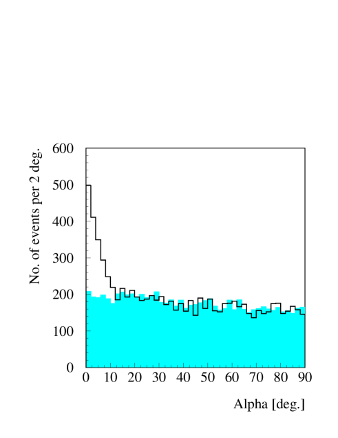
Figure 1: Crab signal observed in 40 h of on-source data taken with the telescope CT3 in stand-alone mode, after cuts on the image parameters width, length, concentration, and distance. Shown is as a full line the distribution in the angle $\alpha$ between the major axis of the Cherenkov image and the direction to the image of the source in the center of the camera. The shaded area indicates the background obtained from an equivalent amount of off-source observations.

The data discussed in the following were taken in Dec. ’96 and Jan. ’97, shortly after the commissioning of the next three telescopes CT4,5,6 and their electronics. During this period, four of the five telescopes (CT3,4,5,6) were operational with the 271-pixel cameras. Three of these used the final 120 Mhz VME Flash-ADC readout; one (CT4) was still equipped with an interim 40 MHz VME Flash-ADC system. The lower sampling frequency results in increased integration times and somewhat higher sky noise for this telescope. The data presented here were taken with a simple two-pixel concidence for the telescope trigger, without a next-neighbor requirement. The fifth system telescope (CT2) was still equipped with an old, coarser 61-pixel camera and CAMAC ADCs. It was operated independently from the other telescopes and is not used in the analysis discussed in the following. The same is true for the smaller prototype telescope CT1. Use of four rather than five telescopes reduces the rate by 20% and 30% for two-telescope and three-telescope triggers, respectively. In addition, for the data set used in the analysis presented here, the central telescope (CT3) was always required among the triggering telescopes, resulting in an additional rate loss of about 25% compared to the normal situation, where any two telescopes would trigger the IACT array.

Given the short time since the data was taken, and the emphasis on continued installation and tests of the hardware, the software algorithms for data analysis as well as our understanding of the properties of the system and its optimization are still imperfect. Also, geometric calibration data were not yet available in sufficient quantity and quality for all telescopes.

Given these various caveats, the following performance figures, though quite remarkable, should not be taken to reflect the ultimate performance of such an array; one should expect detection rates to increase by a factor 1.5 to 2, with a corresponding increase in sensitivity.

2 Triggering of the HEGRA IACT Array

The individual HEGRA telescopes are triggered if two pixels exceed a preset threshold, within a coincidence window of about 12 ns. Presently, any two pixels may trigger the telescope. In future, a hardware next-neighbor unit will require that at least two trigger pixels are direct neighbors, to further reduce the rate of random coincidences. In earlier single-telescope observations, the next-neighbor check was emulated in software, providing a trigger verification after about 100 $\mu$s. This delay is however not compatible with the timing of the multi-telescope coincidence.

The individual telescope trigger signals are routed to a central station, where they are delayed in a custom designed VME unit, to compensate differences in timing which arise since the Cherenkov light front does not reach all telescopes at the same time. The delay values are updated continuously as the source moves across the sky. To trigger the readout of the IACT array, at least two telescopes have to trigger within a time window of 70 ns; this window is large compared to the timing jitter between telescope signals, of order 10 ns. An inter-telescope coincidence causes a global trigger signal and an event number to be transmitted back to all telescopes, including those which did not trigger themselves. After such a global trigger, the Flash-ADCs stop recording signals, the local VME CPU at each telescope locates the appropriate time slice in the Flash-ADC memory, and reads out the data, with on-line sparsification. Data are buffered and multi-event packets are sent via Ethernet to a central event builder station.

Fig. 2 shows the trigger rates for one single telescope (CT3) and for a coincidence of two given telescopes (CT3,4), as a function of the pixel trigger threshold in mV. One photoelectron corresponds roughly to 1.2 mV. For low tresholds, the single-telescope rate shows a very steep dependence on the pixel trigger threshold. In this regime, triggers are almost entirely caused by random coincidences due to night-sky photons; the observed rate is fully consistent with the expected random rate calculated from the measured single-pixel rates and the width of the coincidence window. Only for thresholds above 25 mV the dependence flattens out, and genuine air-shower triggers dominate. In contrast, the two-telescope trigger rate is over the entire range, down to pixel thresholds of 8 mV, governed by air showers, and exihibits a slope similar to the integral cosmic-ray spectrum. For such a trigger, the choice of the pixel thresholds is no longer determined purely by the onset of noise triggers, but rather by other considerations such as the minimal light yield required to generate a useable image.

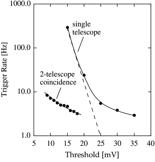
Figure 2: Rate of single-telescope (CT3) triggers and of two-telescope (CT3,4) coincidences, as a function of the pixel trigger threshold applied to the camera pixels. One photoelectron is roughly equivalent to 1.2 mV. The dashed line shows the calculated rate of random single-telescope triggers. The rate of random two-telescope coincidences is small compared to the measured rates.

For any given pixel threshold, the rate of two-telescope (CT3,4) coincidences is smaller than the rate of good single-telescope (CT3) triggers. The reason is twofold: on the one hand the effective area of a two-telescope coincidence is smaller than that of a single telescope, since both telescopes have to be located within the light pool of an air shower. On the other hand, the coincidence requirement provides already at the trigger level a suppression of hadron-induced showers as compared to $\gamma$-ray showers.

Mode	Pixel threshold	Energy threshold
	(photoelectrons)	(TeV)
Single telescope,	$\approx 22$	$\approx 1.0$
any 2 pixels
Single telescope,	$\approx 15$	$\approx 0.7$
two neighbor pixels
4-Telescope system,	$\approx 8$	$\approx 0.5$
at least two telescopes,
any two pixels per telescope

Table 1: Experimentally determined pixel thresholds and resulting energy thresholds for different trigger modes. The pixel thresholds are chosen such that the rate of random 2-pixel coincidences is small (O(10%)) compared to the rate of triggers caused by air showers. The energy thresholds are derived using Monte Carlo simulations; the thresholds refer to $\gamma$-rays and are defined as the energy with the peak differential counting rate for a source with a spectral index similar to the cosmic-ray spectrum, for vertical incidence.

Table 1 summarizes the typical pixel trigger thresholds achieved for the different modes of operation. To relate these pixel thresholds to energy thresholds, a Monte Carlo simulation of the system response is required. Since the detailed Monte Carlo simulation of the system is still under development, a fast simulation tool using parametrized trigger efficiencies was used [16]. Fig. 3 shows the resulting differential detection rates for four cases: (1) the 5-telescope IACT array, (2) the present 4-telescope array with CT3 required in the analysis, in either case with a 2-telescope trigger and a pixel threshold of 8 photoelectrons, (3) the single telescope CT3 with a next-neighbor trigger and a pixel threshold of 15 photoelectrons, and (4) CT3 with a 22 photoelectron threshold. While the fast simulation does not reach the accuracy of a full Monte Carlo simulation, it is expected to reproduce the relative performance rather well.

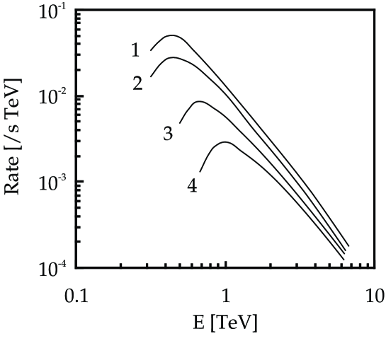
Figure 3: Simulated differential detection rates for a $\gamma$-ray source with a differential spectral index of 2.7 and a flux of $10^{-11}$/cm²s. Curves: (1) full IACT system, 8-photoelectron threshold, (2) IACT system as used in the present analysis, 8-p.e. threshold, (3) single telescope, 15-p.e. threshold, (4) single telescope, 22-p.e. threshold.

One notices that at large energies the effective area and hence the differential detection rate of the system is not much larger than that of a single telescope; the gain in total detection rate results mainly from the lower threshold. The resulting energy thresholds are included in Table 1; they should be reliable within 20%. The threshold for the IACT system is about 1/2 of that of an equivalent (without next-neighbor trigger) single telescope. The 8 photoelectron threshold, which was used for all system data discussed here, results in a global trigger rate of 12 Hz.

Many other aspects of the multi-telescope trigger coincidence have been investigated, such as the dependence of rates on zenith angle or their dependence on the relative pointing of the individual telescopes; more details will be published elsewhere.

3 Calibration and Data Analysis

The analysis of data generated by the HEGRA IACT system builds upon the well-known techniques for image analysis of single-telescope data, augmented by new developments in certain areas, such as an improved geometry calibration of the telescopes, the procedures to extract the amplitude information from the Flash-ADC data, and the techniques for stereoscopic reconstruction.

The stereoscopic reconstruction of air showers, with its resolution in the mrad-range, is very sensitive to deviations in the pointing of the telescopes. In the past, pointing deviations of up to one pixel size were observed for some of the HEGRA telescopes, which is absolutely unacceptable for a proper stereoscopic reconstruction. Alignment procedures developed earlier within HEGRA were extended and refined to cope with this problem. A first step after the installation of a telescope is the alignment of the vertical axis and a survey of the telescope by means of a theodolite. The final alignment is then based on so-called “point runs”. In these runs, the image of a star is scanned in fine lines across one or more pixels, and the DC pixel currents are measured. From those scans, both the center of gravity of the image - and hence any pointing deviations - and the point spread function can be determined. To provide a complete map of pointing deviations, the procedure is repeated with many stars distributed over the entire sky. Figs. 4(a),(b) illustrate the differences between the nominal positions of the stars and their actual images measured using the pixel currents, as a function of altitude and azimuth. These data are then fit to a model of pointing deviations including atmospheric refraction and, as free parameters, the bending of the camera masts (proportional to $\cos(altitude)$), an offset of the camera from the optical axis, a deviation of the azimuth axis from vertical alignment, offsets in the shaft encoder values, and 2nd harmonics for the shaft encoder response, caused e.g. by eccentricity of the axes or gears. This model provides a consistent description of the pointing data; after corrections, all stars appear at their nominal positions, with an rms deviation of less than $0.005^{\circ}$ (Fig. 4(c)). Exact pointing data exist so far only for 3 of the 4 telescopes used here.

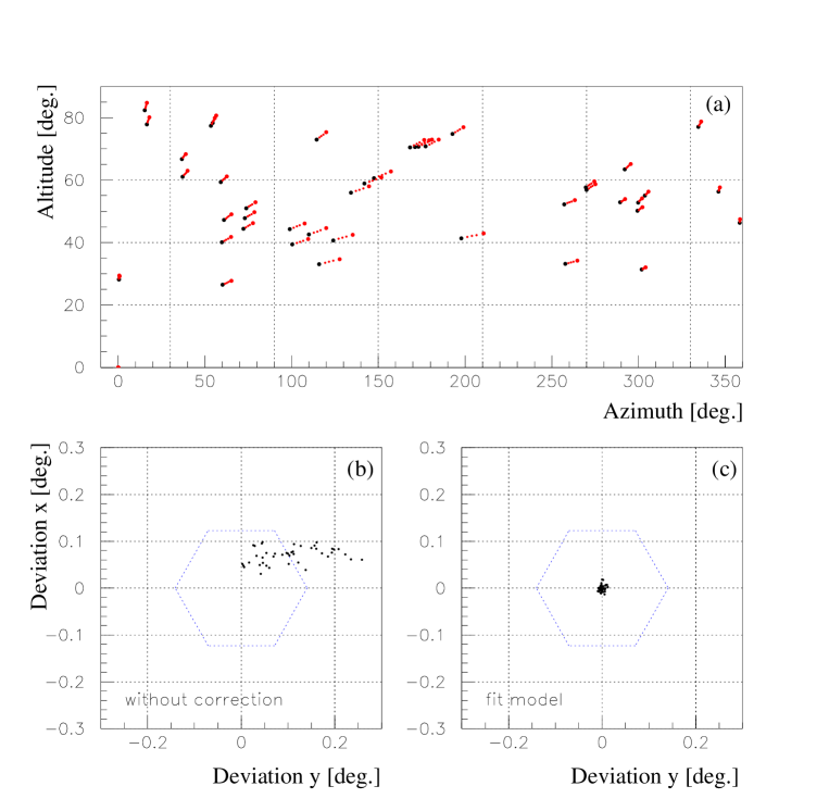
Figure 4: (a) Pointing deviations of one of the HEGRA telescopes as a function of azimuth and altitude, determined using images of bright stars. The (enlarged) deviations are indicated as vectors. (b) Measured deviations from the nominal pointing for an ensemble of stars (in the camera coordinate system). For comparison, the outline of a 0.25^∘ camera pixel is superimposed. (c) Deviations after correction using the model discussed in the text.

While the pointing calibration is repeated rather infrequently - typically a few times per year - calibration data relevant for camera and electronics operation are collected regularly during data taking. In particular, runs with a scintillator light source pulsed by a laser are used to flat-field the camera, and to calibrate pixel timing.

For the analysis for the Flash-ADC data, the following procedure emerged: pedestal values are continuously tracked and updated based on Flash-ADC samples before and after the shower signal. For signals which do not saturate the Flash-ADC dynamic range, the signal is digitally deconvoluted. The deconvolution reverses the effect of signal shapers in front of the Flash-ADC, which are required to suppress signal components above the Nyquist frequency. The deconvolution shortens the signal and hence the effective integration time (Fig. 5), thereby reducing the influence of sky noise. The deconvolution assumes a linear response and cannot be applied to signals saturating the dynamic range of the 8-bit Flash-ADC. For overflow pulses, the area under the truncated pulse (i.e., the sum of the Flash-ADC samples) is still a monotonic function of the amplitude. A look-up table is used to convert the area into an amplitude, extending the linear dynamic range by a factor of more than 2, up to about 500 photoelectrons per pixel.

Figure 5: PMT signal before and after digital deconvolution of the Flash-ADC data, averaged over many pulses.

A conversion factor relating the ADC signal to the number of photoelectrons has been derived with two independent techniques, once using the width of the laser calibration signal (which is essentially governed by photoelectron statistics), and once using a pulsed light source shining a defined amount of light onto the mirror. Both techniques are in good agreement and give about 1 ADC count per photoelectron.

Images are finally analyzed in terms of the usual 2nd-moment parameters, providing the center of gravity of the images, their orientation, and their width and length. A two-level tail cut is used to selected pixels belonging to the image. To be included, a pixel has either to show a signal equivalent to 6 photoelectrons, or to have at least 3 photoelectrons and a neighbor pixel with at least 6 photoelectrons. Images are only accepted if they contain at least one additional pixel adjacent to one of the trigger pixels.

The shower axis and core location are then derived geometrically (see, e.g., [17, 7, 18], and [5]). Both the image of the source and the point where the shower axis intersects the plane of the mirror dish have to lie on the symmetry axis of the image. The shower direction is hence derived by superimposing the images and intersecting their axes (Fig. 6(a)). The core location is obtained by intersecting the image axes emerging from the telescope locations (Fig. 6)(b) (assuming the mirror planes of all telescopes coincide; the extension to the general case is straight forward). At present, the intersection points are calculated for each pair of telescopes, and then averaged over all pairs, weighted according to the angle between the views. Advanced procedures and fits, which properly track the errors of the image parameters, have been developed, but have not yet been applied to the data.

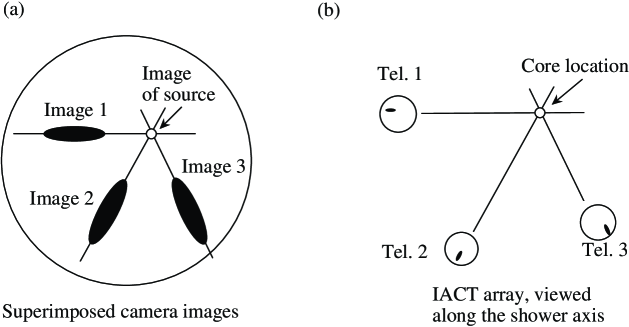
Figure 6: Reconstruction of (a) the shower direction and of (b) the core location from the images observed in the cameras.

First results are also available which use the timing information in the Flash-ADC data for the stereoscopic reconstruction, in addition to the amplitude information; this topic is, however, beyond the scope of this brief report.

4 Performance for Crab Observations

The analysis presented in the following is based on about 11.7 (on-source) hours of observations of the Crab Nebula with the four IACTs CT3,4,5,6. Zenith angles ranged from $5^{\circ}$ to $40^{\circ}$, with a mean value of $20.2^{\circ}$. About half of these data were taken in ON-OFF mode, with equal shares of time on-source and off-source. For the other half, the Crab Nebula was displaced by $0.5^{\circ}$ from the optical axis, and a region displaced symmetrically by the same amount in the opposite direction is used to estimate backgrounds.

Fig. 7 shows the distribution in the direction of reconstructed shower axes, without any additional cuts. An excess from the direction of the Crab Nebula is already visible in this raw data.

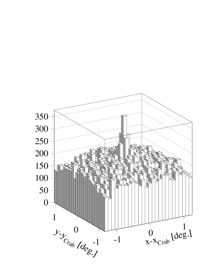
Figure 7: Distribution of the reconstructed shower directions relative to the direction to the Crab Nebula, for events where at least two telescopes triggered, for 11.7 hours of on-source observations, before cuts.

For a quantitative analysis, we plot the distribution in the angle $\theta$ between the shower axis and the direction to the Crab Nebula; shown in Fig. 8 is $dN/d\theta^{2}$. Since $\theta$ is an angle in space, one expects for the uniform background from charged cosmic rays a flat distribution,

$$\left({dN\over d\theta^{2}}\right)_{CR}=const.~{}~{}~{},$$ (1)

whereas a point source at the origin generates an excess

$$\left({dN\over d\theta^{2}}\right)_{Source}\sim e^{-\theta^{2}/2\sigma^{2}}~{}~{}~{}~{},$$ (2)

with the (projected) angular resolution $\sigma$. Fig. 8 illustrates that the distribution of events is indeed flat over a wide range in $\theta^{2}$, with the signal confined to a narrow spike at $\theta\approx 0$.

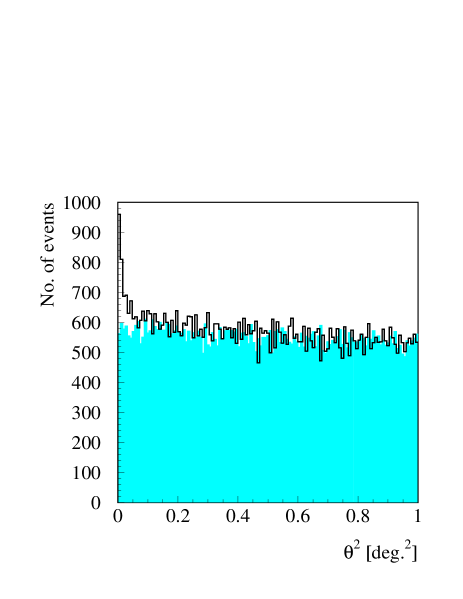
Figure 8: Line: distribution $dN/d\theta^{2}$ of events in the square of the angle $\theta$ relative to the direction to the Crab Nebula. The shaded histogram shows the background derived from off-source runs and analyses with a shifted source position (see text).

It is instructive to compare these (uncut) data with typical data reported for conventional single telescopes - the equivalent plot is the distribution in the angle $\alpha$ between the image axis and the direction to the camera center, i.e., the source (see Fig. 1). In terms of the signal to noise ratio, the uncut system data are not too far from the single-telescope data where tight image cuts have been applied; in the raw single-telescope data the Crab signal is barely visible.

The advantages of the stereoscopic technique are related to the fact the the signal is confined to a small region (about 1%) of the available two-dimensional phase space, whereas in the typical $\alpha$-distribution the signals extend over about 10% of the $\alpha$-range. In particular,

• due to the concentration of the signal events, a highly significant peak is seen already in the 11.7 h of raw system data

• due to the flat distribution of background in two dimensions, the background under the signal can be estimated reliably even without dedicated off-source runs.

Apart from the information concerning the shower direction - for system data, contained directly in the direction reconstructed event-by-event, for single-telescope data contained e.g. in the variable $\alpha$ and the distance $d$ between the image and the camera center - image shapes are used to reject hadronic showers. Relevant image parameters are the width $w$ of the images, their length $l$, the degree of concentration of the image, etc. Figure 9 shows, e.g., the distribution in the mean width $\bar{w}$ - averaged over all telescopes which triggered in a given event - for showers with directions within 0.13^∘ from the Crab. As expected for $\gamma$-ray showers, the excess events have small values of $\bar{w}$.

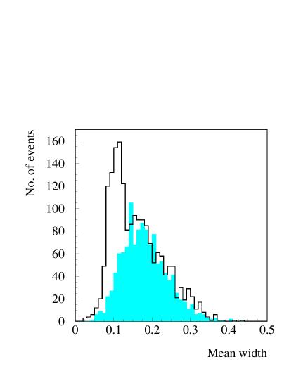
Figure 9: Line: distribution of the mean width $\bar{w}$, averaged over all telescopes which triggered in a given event, for showers from the direction of the Crab Nebula. The shaded histogram shows the background derived from off-source runs and analyses with a shifted source position.

Given that the different image parameters are strongly correlated, and dependent on the amplitude of an image, the optimization of cuts is non-trivial even in the case of a single telescope. The number of parameters increases with the number of telescopes, rendering the problem even more complex. A simple cut e.g. on the widths of all images is a rather inefficient procedure, since some images - those with large amplitudes and optimal distances around 100 m from the shower core - provide a large separation power, whereas faint images differ little between hadronic and photon-induced showers and a cut merely reduces the efficiency for photons, without a corresponding gain in signal-to-noise. Therefore, a different procedure was followed: Monte-Carlo events were used to parametrize the distribution in width $w$ and length $l$ as a function of the nature of the incident particle, of the amplitude $A$ of the image, of the distance $D$ to the shower core, and of the zenith angle $z$ under which the shower was observed. Lacking sufficient Monte Carlo statistics, the joint distribution was factored into a $w$-dependent and a $l$-dependent term, neglecting their correlation:

$$\rho(w,l|A,D,z)=\rho_{w}(w|A,D,z)\rho_{l}(l|A,D,z)~{}~{}~{}.$$ (3)

A ‘probability’ $p$ for a given hypothesis - $\gamma$-ray or cosmic-ray shower - was calculated by multiplying the terms for the individual telescope images $i$, with their image parameters $w_{i}$ and $l_{i}$ and the image amplitude $A_{i}$

$$p=\prod_{i}\rho_{w}(w_{i}|A_{i},D_{i},z)\rho_{l}(l_{i}|A_{i},D_{i},z)~{}~{}~{}~{}.$$ (4)

The distance $D_{i}$ between telescope $i$ and the shower core is calculated using the stereoscopic reconstruction of the core location. Events were then selected by requiring that the ‘probability’ for the $\gamma$-ray hypothesis exceeds the ‘probability’ for the cosmic-ray hypothesis by a certain factor. This procedure avoids the potentially rather inefficient cuts on individual image parameters.

Of course, rather than using Monte-Carlo cosmic-ray events, one can use real events from off-source runs; both choices gave similar performance.

Figs. 10,11 show the directional distribution of events after this cut, with the additional requirement that at least two telescopes have images with 50 or more photoelectrons. The projected rms angular resolution derived from the peak is $0.08^{\circ}$ (Fig. 11); for optimum signal-to-noise, one should hence select a region with a radius of about $0.13^{\circ}$ around the source. Table 2 lists the resulting rates and efficiencies. The shape cuts discussed above allow to reduce comic-ray background by almost a factor 100, while maintaining a 40% efficiency for $\gamma$-rays. With simpler cutting procedures, based e.g. on the mean width $\bar{w}$ of all telescope images, and on their mean length and concentration, background rejection is about a factor 2 worse, but still sizeable.

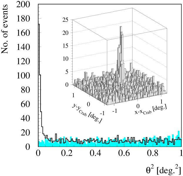
Figure 10: Line: distribution of reconstructed shower directions, relative to the direction to the Crab Nebula, after cuts on the event shapes. The shaded histogram shows the background derived from off-source runs and analyses with a shifted source position. The small insert shows the two-dimensional distribution of shower directions.

Figure 11: Expanded view of the signal region, showing the background-subtracted peak with an exponential fit corresponding to a projected angular resolution of $0.08^{\circ}$.

We note that for short observation times of one hour, one expects about one background event in the signal region, whereas a source with a flux of the Crab generates about 20 events. This features allows e.g. sky surveys with an observation time of about 1 h per $2^{\circ}$ by $2^{\circ}$ region (the effective field of view of the system), at a sensitivity of about 30% of the Crab flux. For longer-term observations - 100 h on-source corresponding to one or two months of data taking - a source of 3% of the Crab flux should still generate a 5-sigma signal, on top of an average background of about 120 events . For comparison, the single telescope CT3 provides a detection limit of 15% to 20% of the Crab flux after 100 h on-source (see Fig. 1). A uniform extended source of diameter $1^{\circ}$ is detectable by the system if the total flux exceeds 15% of the Crab flux, assuming 100 h of on-source data. In this case, an equivalent amount of off-source data is required for background subtraction.

	Before shape cuts	After shape cuts	Selection eff.
Signal	55/h	23/h	0.42
(MC)	(58/h)	(29/h)	(0.5)
Background	105/h	1.2/h	0.011
(MC)	(95/h)	(3/h)	(0.03)

Table 2: Detection rates for Crab observations with the 4-telescope system, before and after shape cuts, and efficiency of the shape cuts. Rates given refer to a circle with radius $0.13^{\circ}$ around the source location. The numbers in parentheses represent Monte Carlo estimates (see text); for the $\gamma$-ray source a flux of $10^{-11}$/cm²s above 1 TeV is assumed, and a differential spectral index of 2.7. For the background, only the cosmic-ray proton component is considered; heavier nuclei have significantly reduced trigger probabilities.

To provide a consistency check, Table 2 also includes Monte Carlo based estimates for the detection rates. For the $\gamma$-ray source a differential spectral index of 2.7 is assumed, and a flux of $10^{-11}$/cm²s above 1 TeV. Recent single-telescope HEGRA measurements give values for the Crab flux above 1 TeV of $(0.8\pm 0.3)\cdot 10^{-11}$/cm² [13] and $1.5^{+1.0}_{-0.5}\cdot 10^{-11}$/cm² [14], with a spectral index of $2.7\pm 0.3$, and $0.77^{+0.47}_{-0.13}\cdot 10^{-11}$/cm² [15] above 1.5 TeV. The raw detection rates given in the table are based on the fast simulation tool using parametrized trigger efficiencies. The Monte Carlo estimates for the rates before cuts should be reliable within 50%. Given these caveats, the agreement of simulated and measured rates before cuts is surprisingly good.

The Monte Carlo selection efficiencies quoted in the table refer to early simulations, which were carried out using a slightly different configuration and different selection criteria, and should only serve to illustrate approximate magnitudes; the cuts used in the present data analysis are obviously somewhat tighter. The angular resolution has been simulated [18] using the identical algorithm used for shower reconstruction, and the predicted value of 0.1^∘ is in good agreement with the measured (projected) resolution of $0.08^{\circ}$ after cuts, or $0.09^{\circ}$ before cuts. (The cuts bias towards well-measured narrow showers, resulting in a slightly improved resolution.)

5 Conclusion

In summary, it seems appropriate to state that while both the hardware of the HEGRA IACT array and the analysis techniques are still evolving and further improvements are to be expected, existing data clearly demonstrate the power and the potential of the stereoscopic approach. The detection rates and angular resolutions are consistent with expectations based on Monte-Carlo studies. Data clearly demonstrate the lower trigger thresholds achievable with a telescope coincidence trigger, the high level of suppression of the cosmic-ray background, and the superior angular resolution.

References

- [1] T.C. Weekes, Space Science Rev. 75 (1996) 1; M. F. Cawley and T.C.Weekes, Experimental Astronomy 6 (1996) 7.
- [2] F. Aharonian, Proceedings of the Int. Workshop “Towards a Major Atmospheric Cherenkov Detector II”, Calgary, (1993), R.C. Lamb (Ed.), p. 81.
- [3] F. Aharonian et al., Experimental Astronomy 2 (1993) 331.
- [4] F. Aharonian et al., Astroparticle Phys. (1997), in press.
- [5] C.W. Akerlof et al., Astrophys. J. 377 (1991) L97.
- [6] S. Le Bohec, Proceedings of the Int. Workshop “Towards a Major Atmospheric Cherenkov Detector IV”, Padua, (1995), M. Cresti (Ed.), p. 378.
- [7] M. Ulrich, Ph.D. Thesis, Heidelberg (1996); M. Ulrich et al., publication in preparation.
- [8] T.C. Weekes et al., Astrophys. J. 342 (1989) 379.
- [9] G. Vacanti et al., Astrophys. J. 377 (1991) 467.
- [10] P. Goret et al., Astron. & Astrophys. 270 (1993) 401
- [11] P. Baillon et al., Astroparticle Phys. 1 (1993) 341.
- [12] T. Tanimori et al., Astrophys. J. 429 (1994) L61.
- [13] A. Konopelko et al., Astroparticle Phys. 4 (1996) 199.
- [14] D. Petry et al., Astron. & Astrophys., 311 (1996) L13.
- [15] S.M. Bradbury et al., Astron. & Astrophys., in press.
- [16] W. Hofmann and C. Köhler, to be published.
- [17] M. Kohnle et al., Astroparticle Physics 5 (1996) 119.
- [18] M. Ulrich, Proceedings of the Int. Workshop “Towards a Major Atmospheric Cherenkov Detector IV”, Padua, (1995), M. Cresti (Ed.), p. 121.