Abstract

Using archival ASCA observations of TT Arietis, X-ray energy spectra and power spectra of the intensity time series are presented for the first time. The energy spectra are well-fitted by a two continuum plasma emission model with temperatures $\sim 1$ keV and $\sim 10$ keV. A coherent feature at $\sim 0.643$ mHz appeared in the power spectra during the observation.

Key words: Subject headings: binaries: close -stars: individual (TT Arietis) -stars: cataclysmic variables -X-rays: stars

Section 1 Introduction

TT Arietis has been categorized as a nova-like variable from photometric observations (Smak & Stepien 1969, Cowley et al., 1975). The system’s spectroscopic orbital period is found to be 0.13755114(13)${}^{d}$ (Thorstensen et al., 1985) from measurements of the radial velocities of emission lines. This is longer than the photometric period of 0.1329${}^{d}$ (Tremko 1992). The beat frequency of the photometric and spectroscopic orbital periods is $\sim 0.25$ d${}^{-1}$ which is very similar to the intermediate polar TV Col (Hellier et al. 1991). This led Jameson et al. (1982) to the suggestion that TT Ari is an intermediate polar. The optical brightness of TT Ari varies irregularly on long time scales. It can remain at visual magnitudes $\sim 10$ (high state) for many years, interrupted irregularly by low states with visual magnitudes $\sim 16$ which last less than a year (Shafter et al. 1985). In the high state, TT Ari has shown flickering activity (or quasi-periodic oscillations) with periods between 14 min and 27 min (Semeniuk et al., 1987; Hollander & van Paradijs 1992).

TT Ari was found to be a hard X-ray source by the Einstein satellite (Cordova et al., 1981). Jensen et al. (1983) investigated the correlation of X-ray and optical flickering activity using simultaneous observations with the Einstein X-ray observatory and the Mount Wilson Optical Telescope. They found that the flickering activity of X-rays at $\sim 17$ min ($\sim 1$ mHz) is delayed by $\sim$ 1 min with respect to the optical flickering activity. They proposed that the optical flickering in TT Ari is produced in the inner accretion disk, and a fraction of the energy is transported to a different region where the X-ray flickering is produced. The 1 min time delay between the optical and X-ray flickering would be the time required to transport energy from the optical flickering region to the X-ray emitting region (Jensen et al., 1983).

In the present work, we analyze archival ASCA data to construct the X-ray egergy spectra and power spectra of TT Ari. Section 2 describes the observations. Section 3 describes the X-ray spectra and X-ray timing.

Section 2 Observations

TT Ari was observed with ASCA on January 20 to 21, 1994 with an effective exposure time $\sim 14$ ksec. The ASCA instrumentation (Tanaka et al. 1994) consists of four imaging telescopes, each with a dedicated spectrometer. There are two solid-state imaging spectrometers (SIS), each consisting of 4 CCD chips, giving an energy resolution of 60-120 eV across the 0.4-10 keV band. The SIS with 2-CCD mode and GIS data were taken with a time resolution 8 sec and 62.5 msec respectively. Two gas scintillation proportional counter imaging spectrometers, GIS, have an energy resolution of 200-600 eV over the 0.8-10 keV band. Data were extracted within a $\sim 4$ arcmin radius region for each SIS and within a $\sim 6$ arcmin region for each GIS. The typical mean count rates of TT Ari, for the SIS and GIS are $\sim 0.59$ and $\sim 0.48$ count sec${}^{-1}$, respectively. Standard cleaning for ASCA data was applied to eliminate X-ray contamination from the bright Earth, effects due to high particle background, and hot flickering SIS pixels. The reduction of the ASCA archival data and the correction of the photon arrival times to the Solar System barycenter was performed using XSPEC, XRONOS, XIMAGE and XSELECT softwares. In Fig. 1, we present the light curve of the observation.

Figure 1: The light curve of TT Ari with SIS0 count rates binned in intervals of 86 sec. The times indicates MJD 40000+.

Section 3 Results

3.1 X-Ray Spectra

The large number of counts obtained from ASCA observations and the broad energy range (0.5-10 keV) allows for fits using various spectral models. The spectrum was fitted with a two component Raymond Smith (1977) emission model as expected from radiatively cooling shock regions. The measured unabsorbed flux during the observation was $\sim 9.74\times 10^{-12}$ erg sec${}^{-1}$ cm${}^{-2}$ in the band of 0.5-10 keV.

In order to see the lower energy part of the spectrum ($<$ 2 keV) more clearly and to estimate the column density N${}_{H}$ more accurately, ROSAT archival observations of TT Ari were extracted and a two component Raymond-Smith model was fitted to combined ASCA and ROSAT data. Our preliminary analysis showed that both data sets have similar spectra. In these fits, we assume that the spectral parameters of ASCA and ROSAT observations were the same up to a normalization factor. Results of the fit, shown in Table 1, imply that the ASCA flux was $1.1\pm 0.02$ of the ROSAT flux. The column density of N${}_{H}\sim(4.13\pm 0.11)\times 10^{20}$ cm${}^{-2}$ obtained from the joint fit of the ROSAT and ASCA data sets is consistent with the previously deduced value from the ROSAT observation alone (Baykal et al., 1995). The two component Raymond Smith model fits the data well with $\chi^{2}_{\nu}\sim 1.03$, giving the plasma temperatures of about $\sim 1$ keV and $\sim 10$ keV, for the two components.

Keeping in mind that the spectral characteristics may change in time and while the column density probably remains constant; the column density deduced from the joint ROSAT-PSPC and ASCA-SIS0+GIS2 data was used for further spectral work with the ASCA observations. In Fig. 2, we present the energy spectra fits with the two component model. Only SIS0+GIS2 data are used for clarity.

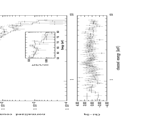
Figure 2: The average ASCA/ SIS0, GIS2 spectra of TT Ari. The upper panel shows the fit of the two component Raymond-Smith model. Data is binned for 5$\sigma$ confidence. The lower panel is the $\chi^{2}$ residuals from the fit. Inset shows 6.67 keV feature, binned for 3$\sigma$ confidence, together with the model fitted to it.

Table 1 gives the spectral parameters for the best fit to the SIS0+GIS2 data to compare with the joint fit and two component Raymond Smith model to SIS0+SIS1+GIS2+GIS3 detectors.

Table I: Spectral Fit Parameters for Two Temperature Models ${}^{a}$

model	kT${}_{1}$(keV)	kT${}_{2}$(keV)	A${}_{1}(10^{-4}$)${}^{f}$	A${}_{2}(10^{-3}$)${}^{f}$	N${}_{H}(10^{20}$cm${}^{-2}$)	$\chi^{2}_{\nu}$
R-S ${}^{b}$	$1.03\pm 0.05$	$10.99\pm 1.17$	$4.92\pm 1.36$	$6.83\pm 0.14$	$4.13\pm 0.11$	1.03
R-S ${}^{c}$	$0.99\pm 0.12$	$9.29\pm 1.02$	$3.70\pm 2.22$	$7.16\pm 0.19$	4.13 fixed	0.96
R-S ${}^{d}$	$0.97\pm 0.08$	$8.49\pm 0.63$	$3.67\pm 1.51$	$7.26\pm 0.13$	4.13 fixed	1.36
Meka ${}^{e}$	$0.76\pm 0.05$	$8.10\pm 0.49$	$3.37\pm 0.91$	$7.32\pm 0.09$	4.13 fixed	1.48

${}^{a}$ Spectral fits were performed using the program XSPEC.
  ${}^{b,c,d}$ Raymond$-$Smith model for PSPC+SIS1+GIS2, SIS1+GIS2 and SIS0+SIS1+GIS2+GIS3 detectors respectively.
  ${}^{e}$ Mewe$-$Kaastra model for SIS0+SIS1+GIS2+GIS3 detectors.
  ${}^{f}$  A${}_{1}$ and A${}_{2}$ are the emission measures in units of $10^{-14}/(4\pi D^{2})\int~{}~{}n^{2}dV$, where $D$ is the distance
to the source (cm) and n is the electron density (cm${}^{-3}$).