The Delayed Formation of Dwarf Galaxies

Abstract

One of the largest uncertainties in understanding the effect of a background UV field on galaxy formation is the intensity and evolution of the radiation field with redshift. This work attempts to shed light on this issue by computing the quasi-hydrostatic equilibrium states of gas in spherically symmetric dark matter halos (roughly corresponding to dwarf galaxies) as a function of the amplitude of the background UV field. We integrate the full equations of radiative transfer, heating, cooling and non-equilibrium chemistry for nine species: H, H⁺, H^-,H₂, H${}_{2}^{+}$, He, He⁺, He⁺⁺, and e^-. As the amplitude of the UV background is decreased the gas in the core of the dwarf goes through three stages characterized by the predominance of ionized (H⁺), neutral (H) and molecular (H₂) hydrogen. Characterizing the gas state of a dwarf galaxy with the radiation field allows us to estimate its behavior for a variety of models of the background UV flux. Our results indicate that a typical radiation field can easily delay the collapse of gas in halos corresponding to 1-$\sigma$ CDM perturbations with circular velocities less than $30~{}{\rm km~{}s^{-1}}$.

1 Introduction

How do galaxies form? Most models predict that galaxies are assembled through a successive series of mergers of smaller systems, a process known as hierarchical clustering. These models also predict that small galaxies form before big galaxies. Observations, however, suggest the opposite: while low mass galaxies are forming the bulk of their stars at $z\sim 1$ (Driver et al (1995); Babul & Ferguson (1996)), large galaxies appear to be well-established by $z\sim 1$ and do not show significant evolution between $z\sim 1$ and today in luminosity, color, size or space density (Steidel & Dickinson (1994); Steidel, Dickinson & Persson (1994)).

The resolution of this apparent conflict between theory and observations may lie in the physics of galaxy formation: the hierarchical clustering paradigm only describes the formation of gravitationally bound entities, not the process of converting gas into stars. Observations of Ly$\alpha$ clouds along quasar lines-of-sight suggest that at high redshifts, the universe is permeated by a metagalactic UV flux that may suppress star formation by rapidly dissociating atomic and molecular gas. At $z=2$, this background is estimated to have a strength $J_{\nu}\approx 10^{-21}$ erg s^-1 cm^-2 ster^-1 Hz^-1 at the Lyman limit (Bechtold et al (1987)). As discussed by Babul & Rees (1992) (see also Efstathiou (1992)), an ionizing flux of such intensity can easily prevent the gas in low mass halos from settling and forming stars. Analytic calculations (Rees (1986); Ikeuchi (1986)) suggest that the halos affected will be those with circular velocities $v_{c}<30~{}{\rm km~{}s^{-1}}$, a result confirmed by recent numerical studies (Katz, Weinberg & Hernquist (1996); Navarro & Steinmetz (1996); Thoul & Weinberg (1996)).

Although the epoch-dependence of the UV flux is uncertain, it is expected that $J_{\nu}$ declines with redshift. A declining $J_{\nu}$ has two effects on the gravitationally bound, photoionized gas in the halos. First, the rate at which the gas is photoheated will decrease and hence, its equilibrium temperature will also decrease slightly. The reduced temperature results in a gradual concentration of the gas towards the center (Ikeuchi, Murakami & Rees (1989)). Second, the gas becomes more neutral and offers a greater optical depth to the ionizing photons leading to a diminution of the ionizing flux reaching the central regions and the formation of a warm ($T\approx 9000$ K) shielded neutral core (Murakami & Ikeuchi (1990)). The formation of a neutral core, however, is not a sufficient condition for star formation. For a gas cloud to be susceptible to star formation, it must be at least marginally self-gravitating (e.g., Matthews (1972)) and this can occur only if the gas in halos with $v_{c}<30~{}{\rm km~{}s^{-1}}$ can cool below $9000$ K.

Further cooling of a neutral metal-poor gas requires the formation and survival of molecular hydrogen. The formation of molecular hydrogen in a gas of primordial composition occurs via gas phase reactions. Various studies have shown that an external photoionizing radiation field can greatly affect the efficiency of formation of H₂ molecules (Shapiro & Kang (1987); Haiman, Rees & Loeb 1996a ; Haiman, Rees & Loeb 1996b ), with even a moderate UV flux being capable of suppressing the H₂ abundance. In time, however, the decline in the UV intensity will result in the formation of sufficient molecular hydrogen to allow the gas in the halos to cool and become susceptible to star formation. Babul & Rees (1992) argued for $z=1$ as the epoch of galaxy formation in low mass halos, and sought to identify these forming galaxies with the numerous small faint blue galaxies seen in deep images.

In this paper, we present a more thorough investigation of the epoch of galaxy formation in smaller halos with circular velocities in the range $15~{}{\rm km~{}s^{-1}}<v_{c}<70~{}{\rm km~{}s^{-1}}$. Specifically, we only consider halos that form after the metagalactic UV flux has been established ($z<5$). Through a detailed study of the thermal and ionization structure — we take into account radiation transfer, as well as heating, cooling and the corresponding non-equilibrium chemistry (Abel et al (1996); Anninos et al (1996)) for nine species: H, H⁺, H^-, H₂, H${}_{2}^{+}$, He, He⁺, He⁺⁺, and e^- — of the hydrostatic-equilibrium configuration of halo gas subject to a range of UV intensities, we determine the threshold UV intensity at which molecular hydrogen begins to form. Given a specific model for the evolution of the UV flux, the threshold intensity can be easily converted into a redshift of galaxy formation.

In §2 of this paper, we describe the dwarf galaxy model, which includes: the dark matter halos, the amount of gas expected in these halos, the details of the radiative transfer, heating, cooling and non-equilibrium chemistry, and the numerical method. §3 Discusses the results of our simulations. §4 Gives our conclusions.

2 Dwarf Galaxy Model

The current numerical models can not yet incorporate the wide range of physical processes and physical scales associated with galaxy formation. We focus on the quasi-hydrostatic evolution of a gas cloud in a small dark matter halo. By simplifying the problem to the time evolution of a spherically symmetric cloud in a dark matter halo, we were able to incorporate the non-equilibrium chemistry and treat the radiative transfer in much greater detail.

2.1 Dark Matter Halo

We will simulate the evolution of the gas in a fixed halo potential. For our purposes, the dark matter halo is specified by two parameters: the circular velocity $v_{c}$ and the virialization redshift $z_{v}$, which can be translated into a halo radius $r_{{\rm halo}}$ and halo mass $M_{{\rm halo}}$ if we assume that the overdensity at virialization is $\delta\sim 175$ (Gunn & Gott (1972))

$$v_{c}^{2}=\frac{GM_{{\rm halo}}}{r_{{\rm halo}}}~{},~{}~{}~{}\frac{4\pi}{3}r_{{\rm halo}}^{3}\delta\rho_{c}(z)=M_{{\rm halo}},$$ (1)

where the mean density is given by the usual expressions for a $\Omega=1$ CDM cosmological model: $\rho_{c}(z)=(1+z)^{3}\rho_{c}^{0}$, $6\pi G\rho_{c}t_{{\rm Hubble}}^{2}=1$, $t_{{\rm Hubble}}^{0}=2/3H_{0}$.

We will focus on the evolution of “typical” halos, which correspond to 1-$\sigma$ perturbations. In a $b=1.6$ standard CDM model, Press-Schechter theory implies that the halos virialized at a redshift given by

$$1+z_{v}\approx(7.5/1.7)(M_{{\rm halo}}/10^{9}~{}{{\rm M}_{\sun}})^{0.1}~{},~{}~{}~{}10^{8}~{}{{\rm M}_{\sun}}<M_{{\rm halo}}<10^{10}~{}{{\rm M}_{\sun}}$$ (2)

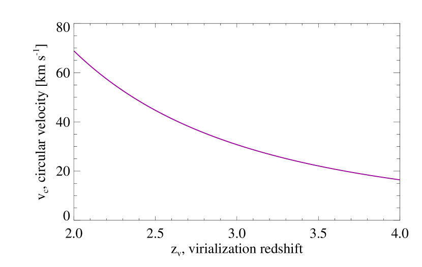
Figure 1: Circular velocity as a function of virialization redshift for 1-$\sigma$ perturbations as computed from Press-Schecter theory using standard CDM.

Figure 1 shows the relationship between halo circular velocity and the virialization epoch for the 1-$\sigma$ perturbations. The basic trend is generic to all hierarchical models: small objects form first and larger objects form later.

We use a dark matter halo profile that has been fit by Burkert (1995) to galaxy rotation curves,

$$\rho_{{\rm DM}}(r)=\frac{r_{0}}{(1+x)(1+x^{2})}~{},~{}~{}~{}x=r/r_{0}$$ (3)

which in turn can be related to the halo radius and mass by

$$r_{{\rm halo}} = 3.4r_{0},$$

$$M_{{\rm halo}} = M_{{\rm DM}}(r_{{\rm halo}}),$$

$$M_{{\rm DM}}(r) = \int_{0}^{r}\rho_{{\rm DM}}(r)4\pi r^{2}dr.$$ (4)

While recent numerical work suggests that the halo density profiles of large galaxies are proportional to $r^{-1}$ in the centers and $r^{-3}$ at the edges (Navarro, Frenk & White (1996)), these profiles do not fit the dwarf galaxy observations (Moore (1994); Flores & Primack (1994)).

2.2 Gas Content and Profile

The ultraviolet background is able to heat the gas to a temperature of roughly $10^{4}~{}\arcdeg$K. In large halos, where $v_{c}>50~{}{\rm km~{}s^{-1}}$, the gas pressure is relatively unimportant and the gas content is determined by the global value of $\Omega_{b}$: $M_{{\rm gas}}=\Omega_{b}M_{{\rm halo}}$ (assuming $\Omega=1$). However, for smaller halos collapsing out of a hot IGM the gas pressure resists the collapse (Thoul & Weinberg (1996)) and $M_{{\rm gas}}<\Omega_{b}M_{{\rm halo}}$. We now make some simple estimates as to where this transition occurs and how much gas should reside in the halo. If the gas in the uncollapsed halo is greater than the Jeans mass than the gas should collapse of its own accord. This provides an upper limit to amount of gas in the halo

$$M_{{\rm gas}}=\Omega_{b}M_{{\rm halo}}~{},~{}~{}~{}\Omega_{b}M_{{\rm halo}}>M_{{\rm Jeans}}$$ (5)

where $M_{{\rm Jeans}}=f\Omega_{b}rho_{c}(2\pi c_{{\rm IGM}}t_{{\rm Hubble}})^{3}$, $f=3/\pi\sqrt{2}$, $c_{{\rm IGM}}^{2}=1.5k_{B}T_{{\rm IGM}}/\mu$. For $\Omega_{b}M_{{\rm halo}}<M_{{\rm Jeans}}$ we can formulate an upper limit for $M_{{\rm gas}}$ by estimating the amount of mass that could be acreted via Bondi accretion in a Hubble time. Thus,

$$M_{{\rm gas}}=M_{{\rm Bondi}}~{},~{}~{}~{}\Omega_{b}M_{{\rm halo}}<M_{J}$$ (6)

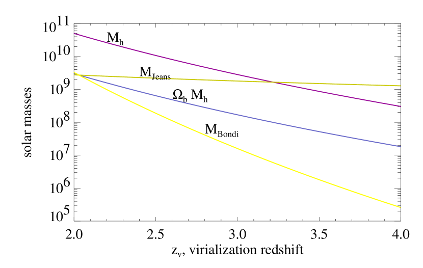
Figure 2: $M_{{\rm halo}}$, $\Omega_{b}M_{{\rm halo}}$, $M_{{\rm Jeans}}$, and $M_{{\rm Bondi}}$ for 1-$\sigma$ perturbations collapsing out of a $20,000~{}\arcdeg$K IGM.

where $M_{{\rm Bondi}}=ft_{{\rm Hubble}}\dot{M}_{{\rm Bondi}}$, $\dot{M}_{{\rm Bondi}}=\pi G^{2}M_{{\rm halo}}^{2}\rho_{c}/c_{{\rm IGM}}^{3}$. Note, the $O(1)$ factor $f$ has been included in $M_{{\rm Jeans}}$ and $M_{{\rm Bondi}}$ so that $M_{{\rm Jeans}}=M_{{\rm Bondi}}$ when $\Omega_{b}M_{{\rm halo}}=M_{{\rm Jeans}}$. Plots of these various masses as function of redshift are shown in Figure 2 for $T_{{\rm IGM}}=20,000~{}\arcdeg$K, indicating that the halos become more DM dominated as they get smaller, which is consistent with the observations (Carignan & Freeman (1988); de Blok & McGaugh (1996)).

The initial gas density profile is specified by hydrostatic equilibrium and by our assumption that the gas is in thermal equilibrium with the background radiation field. This approximation will hold as long as the gas has time to react to changes in the DM potential, self-gravity, and cooling. The scales governing these processes are the sound speed, Hubble time, Jeans mass, and the net cooling/heating time. The sound speed of a $10^{4}~{}^{\circ}$K gas is $\sim 15~{}{\rm km~{}s^{-1}}$, corresponding to a crossing time for a typical $r_{{\rm halo}}\sim 10~{}{\rm kpc}$ halo of $\sim 6\times 10^{8}$ years. The DM potential will change on the order of a Hubble time, which at $z\sim 3$ is $\sim 2\times 10^{9}$ years. The gas will be stable to self-gravity if it is less than the Jeans mass, which from Figure 2 is true for nearly the entire range of models. The heating/cooling time becomes important only when a significant amount of ${{\rm H}_{2}}$ has formed, and determining this point one of the goals of this paper.

2.3 Non-Equilibrium Chemistry

The important role of the detailed chemistry of primordial gas (in particular the formation of ${{\rm H}_{2}}$) has been known and studied since it was first proposed as a mechanism for the formation of globular clusters (Peebles & Dicke (1968)). The potential number of reactions in this simple mixture of H and He is enormous (Janev (1987)). Abel et al (1996) have selected a subset of these reactions to model the behavior of primordial gas for low densities ($n<10^{4}$) over a range of temperatures ($1^{\circ}$K $<T<10^{8}~{}^{\circ}$K); these equations (see Appendix A) represent a careful balance between computational efficiency and accuracy.

2.4 Radiative Transfer

Fully 3D radiative transfer requires estimating the contribution to the flux at every point from every other point along all paths for each wavelength. At the minimum this is a 6D problem. However, in most instances symmetries can be introduced which result in a more tractable situation. The simplest situation occurs when the gas can be assumed to be optically thin throughout. This approximation is sufficient in the majority of cosmological situations (Katz, Weinberg & Hernquist (1996); Navarro & Steinmetz (1996); Anninos et al (1996)) and only breaks down in the cores of halos that have undergone sufficient cooling, a situation that is usually made further intractable by the complexities of star formation. The next simplest geometry is that of a slab (or a sphere under the assumption of a radially perpendicular radiation field), which leaves an intrinsically 2D problem. This approach is the most common in radiative transfer and has been used to address similar situations (Haiman, Rees & Loeb 1996a ; Haiman & Loeb (1996)). Although this approach may not be a bad approximation for a sphere in an isotropic radiation field, we choose to account for all the different paths that penetrate a given spherical shell, which leaves an inherently 3D problem. Although this geometry can significantly increase the size of the computations, for a static grid (i.e. non-adaptive) pre-computing of the various geometric factors can significant alleviate this situation (see Appendix B). Taking into account the different paths effectively “softens” the optical depth, smoothing out transitions from optically thin to optically thick regimes. In addition, introducing the accounting for the different paths lays the groundwork for exploring more general geometries.

2.5 Heating and Cooling

Perhaps the most important aspect of the model is the balance between the heating and cooling processes. This balance is what allows the establishment of a quasi-static temperature profile for a specific radiative flux. If the balance between the heating and cooling is not established, then the hydrostatic equilibrium solution to the gas profile will evolve too rapidly. Fortunately, this situation only comes about when the gas in the halo becomes dense and a large amount H₂ is formed. As was mentioned earlier, this point presumably marks the onset of star formation, which is one of the central goals of this work.

The temperature profile is evolved via the heating and cooling functions found in Anninos et al (1996)

$$\frac{\dot{T}}{T}=\frac{\Gamma(T)-\dot{E}(T)}{E{T}}$$ (7)

where $E=1.5k_{B}T\sum n_{i}$, $i={{\rm e}^{-}},{{\rm H}},{{\rm H}^{+}},{{\rm H}^{-}},{{\rm H}_{2}},{{\rm H}_{2}^{+}},{{\rm He}},{{\rm He}^{+}},{{\rm He}^{++}}$. $\Gamma$ includes photoionizaton heating and $\dot{E}$ includes cooling due to collisional excitation, collisional ionization, recombination, molecular hydrogen, bremsstrahlung and Compton cooling. All the appropriate functions are taken from Appendix B of Anninos et al (1996).

2.6 Numerical Method

The microphysical processes couple to the larger scale density profile primarily through radiative heating, which sets the temperature profile. The rate of radiative heating is in turn strongly dependent on the column densities of each species, which is set by the temperature. Thus, we have a system which is described by differential equations on the small scale with integral constraints on the large scale. The difficulty of solving such a system in the large variety of time scales involved. Solving the entire set simultaneously is prohibitive. Our approach has been to use code modules which solve for each of the processes independently. Iterating between the modules then provides adequate approximation to the true solution. The species solver and heating/cooling modules were provided by Yu Zhang and Mike Norman of NCSA (Abel et al (1996); Anninos et al (1996)). The radiative transfer and hydrostatic equilibrium modules we wrote ourselves. Our central goal is to see how the gas behaves as a function of the amplitude of the background UV field. The overall approach is to pick a halo, set an initial value of $J_{0}$, and estimate the time and number of steps to integrate at this value. We then use each module at each time step which converges on the overall solution. Each module was tested and verified independently. In addition, where possible, combinations of the modules have been tested. A more detailed description of our numerical method is given in Appendix C.

3 Results and Discussion

The goal of the simulation is to determine the maximum ionizing flux that permitted the formation of molecular gas (and stars). The simulations began with the gas ionized. Over the range of objects, the state of the core exhibits the same qualitative behavior (see Figure 3). As the flux decreases the core goes through three phases ionized H⁺ ($T_{{\rm core}}\sim 20,000^{\circ}$K), neutral H ($T_{{\rm core}}\sim 10,000^{\circ}$K) and molecular H₂ ($T_{{\rm core}}\sim 100^{\circ}$K).

In the initial H⁺ state, the object is completely ionized and resembles the IGM. In the H state the core is neutral and the object is like an inverse Stromgren sphere, except that the ionization is primarily collisional, a result of the high temperature maintained by the radiative heating. In the H₂ state, conditions allow for the formation of molecular hydrogen in the core; consequently, the cooling time becomes much less than the dynamical time and the core collapses.

Five simulations were conducted for halos in the range $15~{}{\rm km~{}s^{-1}}<v_{c}<70~{}{\rm km~{}s^{-1}}$ corresponding to: $3\times 10^{8}~{}{{\rm M}_{\sun}}<M_{{\rm halo}}<5\times 10^{10}~{}{{\rm M}_{\sun}}$, $4>z_{v}>2$ , and $3\times 10^{5}~{}{{\rm M}_{\sun}}<M_{{\rm gas}}<3\times 10^{9}~{}{{\rm M}_{\sun}}$ (see Figure 2). For each object there are fluxes $J_{{{{\rm H}}},{{{\rm H}_{2}}}}$ at which the upper transition H⁺ $\rightarrow$ H and the lower transition H $\rightarrow$ H₂ occur (see Figure 4). $J_{{{{\rm H}}},{{{\rm H}_{2}}}}(z_{v})$ can be fit by a formula

$$\ln[J_{{{{\rm H}}},{{{\rm H}_{2}}}}/J_{21}]=a_{{{{\rm H}}},{{{\rm H}_{2}}}}-b_{{{{\rm H}}},{{{\rm H}_{2}}}}z_{v}~{},$$ (8)

where $a_{{{{\rm H}}},{{{\rm H}_{2}}}}=(17.9,17.3)$, and $b_{{{{\rm H}}},{{{\rm H}_{2}}}}=(6.2,6.4)$

Knowing $J_{{{{\rm H}}},{{{\rm H}_{2}}}}$ allows us to place bounds on the behavior of an object in a given radiation field. Most significantly, if the radiation field is above $J_{{{\rm H}}}$, then it will be impossible for the object to collapse and form stars. If the radiation field is below $J_{{{\rm H}_{2}}}$, then it must collapse. Most likely the actual value of the flux at which collapse occurs is between $J_{{{\rm H}}}$ and $J_{{{\rm H}_{2}}}$.

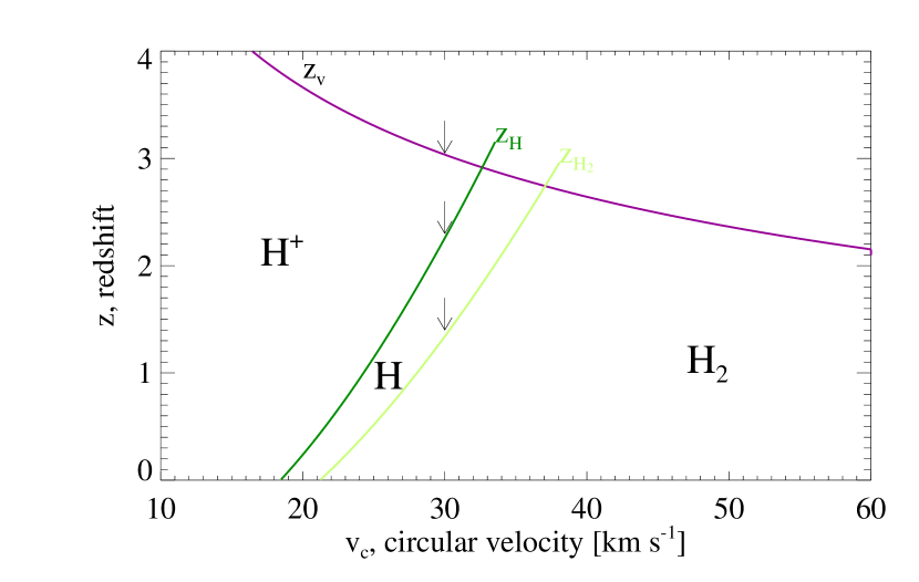
Figure 5: This figure shows the collapse redshift, $z_{v}$, the redshift of H formation, $z_{{{\rm H}}}$, and the redshift of ${{\rm H}_{2}}$ formation, $z_{{{\rm H}_{2}}}$, as a function of the circular velocity of $v_{c}$. Thus, a 1-$\sigma$ perturbation with $v_{c}=30~{}{\rm km~{}s^{-1}}$ collapses at $z\approx 3$ (top arrow), but is ionized until $z\approx 2.5$ (middle arrow) and cannot form molecular hydrogen until $z\approx 1.5$ (bottom arrow). The ionizing field evolves as $J(z)=J_{0}[(1+z)/4]^{4}$, for $z<3$ and $J(z)=J_{0}$, for $z>3$ with the spectral index held fixed at $\alpha=1$. This figure is for a flux amplitude of $J_{0}=10^{-21}$.

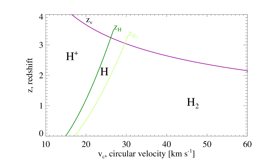
Figure 6: Same as previous figure, but with $J_{0}=10^{-22}$.

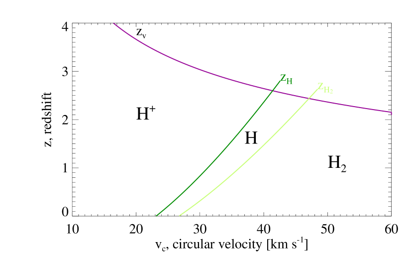
Figure 7: Same as previous figure, but with $J_{0}=10^{-20}$.

For objects consistent with 1-$\sigma$ perturbations in a standard CDM cosmology selecting the evolution of the radiation field ($J(z,\nu)$) specifies critical redshifts $z_{{{{\rm H}}},{{{\rm H}_{2}}}}$ such that for $z_{{{\rm H}_{2}}}<z<z_{{{\rm H}}}$ the object will be in the neutral H state. Figures 5, 6 and 7 plot the virial redshift and the critical redshifts as a function of the circular velocity for three different amplitudes of an evolving UV field

$$J(z,\nu)=\left\{\begin{array}[]{c@{\quad,\quad}c}J_{0}~{}[(1+z)/4]^{4}~{}(\nu_{Ly}/\nu)&z<3\\ J_{0}~{}(\nu_{Ly}/\nu)&z>3\end{array}\right.~{}.$$ (9)

These results indicate that a typical radiation field can easily prevent gas in halos with $v_{c}<30~{}{\rm km~{}s^{-1}}$ from collapsing. Furthermore, the less massive halos, which are typically the first to virialize, are the last to form galaxies. Thus, if these results have any correspondence to observed dwarf galaxies, they suggest that the larger objects will burst earlier, and perhaps will show an observable trend of increasing age with mass.

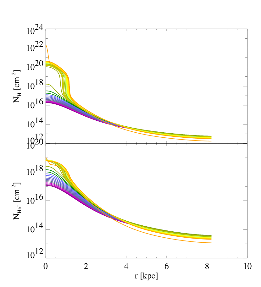
Figure 8: Evolution of the column density profiles of H (top panel) and He⁺ (bottom panel) of the same object shown in Figure 3.

Another important aspect of these objects is their potential contribution to Quasar absorption lines. Figure 8 shows the column density evolution for H and ${{\rm He}^{+}}$. During the ${{\rm H}^{+}}$ phase $N_{{\rm H}}\sim 10^{16-17}$, suggesting that these objects may make a contribution to the Ly$\alpha$ forest and Ly limit systems. During the ${{\rm H}}$ phase $N_{{\rm H}}$ increases dramatically to levels near those seen in damped Ly$\alpha$ clouds, ($N_{{\rm H}}\sim 10^{21}$) but this is probably a relatively short lived phase and therefore is it unlikely that these objects would be seen in Quasar spectra.

Our calculations ignored the role of metals in the evolution of the gas. Metals can have a number of important effects on the chemistry and dynamics of gas clouds: dust grains will absorb ionizing radiation and serve as formation sites for molecular hydrogen and atomic lines of C and other heavy elements can be important coolants at temperatures around $10^{4}~{}^{\circ}$K. Are these processes important in dwarf galaxies at high redshift? Observations of QSO Lyman forest clouds suggest that the metal abundances in meta-galactic gas was $Z\sim 0.001-0.01$ times the solar value at $z\sim 3$ (Songaila & Cowie (1996)). At these abundances, heavy element cooling is unimportant (Bohringer & Hensler (1989)). If we make the conservative assumption that most of the carbon at high redshift is incorporated into dust grains (as in our galaxy), with a size distribution that is similar to the local ISM, then this suggests a cross-section per hydrogen atom of $\sigma_{\rm dust}(1000\AA)\approx Z~{}2\times 10^{-21}~{}{\rm cm}^{2}$ (Draine & Bertoldi (1996)). In our models, the maximum column density occurs when the cloud is most centrally condensed, which occurs just before the onset of ${{\rm H}_{2}}$ formation and is roughly $N_{{\rm H}}\sim 10^{21}~{}{\rm cm}^{-2}$ (see Figure 8). Thus the maximum optical depth at these wavelengths is approximately $\tau_{\rm dust}\sim Z\sim 0.01$. The contribution of dust to ${{\rm H}_{2}}$ formation in our galaxy can be approximated by a ${\dot{n}}_{{\rm H}_{2}}\approx Rn{n_{{\rm H}}}$, where $R=6\times 10^{-18}T^{1/2}~{}{\rm cm}^{3}~{}{\rm s}^{-1}$ (Draine & Bertoldi (1996)). If we scale $R$ by the metallicity, then the dust term will be negligible in comparison to the other terms contributing to ${{\rm H}_{2}}$ formation whenever ${n_{{\rm H}^{-}}}>10^{-9}$, which is nearly always the case in the neutral H core.

4 Conclusions

In this paper, we have studied the evolution of a proto-dwarf galaxy exposed to the metagalactic radiation field. We begin with an ionized gas cloud, initially Jeans stable, in a dark matter halo and follow its hydrostatic evolution as the meta-galactic flux decreases. Our calculations indicate that the state of the gas can be characterized by the predominance of ionized, neutral, or molecular hydrogen in the core. The transitions between these phases takes place quickly as the amplitude of the background flux decreases. We have computed the critical fluxes at which the transitions take place $J_{{{{\rm H}}},{{{\rm H}_{2}}}}$, which serves as upper and lower bounds on the flux at which rapid cooling and the subsequent star formation can begin. If the flux is greater than $J_{{{{\rm H}}}}$, then is unlikely that the gas will cool. If the flux is less that $J_{{{{\rm H}_{2}}}}$, then the gas must cool.

Characterizing the state of the gas in terms of the background flux allows us to use any model for the evolution of flux with redshift. Using typical values of the flux, our simulations indicate that gas in a $v_{c}=30~{}{\rm km~{}s^{-1}}$ halo collapsing at $z\approx 3$ can easily be prevented from forming significant amounts of ${{\rm H}_{2}}$ until $z\approx 2$. Thus our calculations are consistent with photoionization delaying the formation of low mass galaxies (Babul & Rees (1992)).

In this paper we have focused on 1-$\sigma$ perturabtions, in subsequent work we will expand our exploration of the ($v_{c}$,$z_{v}$) plane, which will allow us to further address the issues pertaining to the observed faint blue galaxies. As an example, our preliminary calculations indicate that a $v_{c}=30~{}{\rm km~{}s^{-1}}$ halo which virializes at $z_{v}=2$ will first be able to form neutral H at $z\approx 1.25$.

Appendix A Non-equilibrium Chemistry

The evolution of the electron, hydrogen and helium abundances are computed from the following set of coupled equations (Abel et al (1996)):

$${\dot{n}}_{{\rm H}} = k_{2}{n_{{\rm e}^{-}}}{n_{{\rm H}^{+}}}-(k_{1}{n_{{\rm e}^{-}}}+k_{20}){n_{{\rm H}}}$$ (A1)

$${\dot{n}}_{{\rm H}^{+}} = -{\dot{n}}_{{\rm H}}$$ (A2)

$${\dot{n}}_{{\rm He}} = k_{4}{n_{{\rm e}^{-}}}{n_{{\rm He}^{+}}}-(k_{3}{n_{{\rm e}^{-}}}+k_{21}){n_{{\rm He}}}$$ (A3)

$${\dot{n}}_{{\rm He}^{+}} = -{\dot{n}}_{{\rm He}}-{\dot{n}}_{{\rm He}^{++}}$$ (A4)

$${\dot{n}}_{{\rm He}^{++}} = k_{5}{n_{{\rm e}^{-}}}{n_{{\rm He}}}-k_{6}{n_{{\rm e}^{-}}}{n_{{\rm He}^{++}}}+k_{22}{n_{{\rm He}^{+}}}$$ (A5)

$${n_{{\rm H}^{-}}} = \frac{k_{7}{n_{{\rm e}^{-}}}{n_{{\rm H}}}}{(k_{8}+k_{15}){n_{{\rm H}}}+(k_{16}+k_{17}){n_{{\rm H}^{+}}}+k_{14}{n_{{\rm e}^{-}}}+k_{23}}$$ (A6)

$${\dot{n}}_{{\rm H}_{2}} = k_{8}{n_{{\rm H}^{-}}}{n_{{\rm H}}}+k_{10}{n_{{\rm H}_{2}^{+}}}{n_{{\rm H}}}+k_{19}{n_{{\rm H}_{2}^{+}}}{n_{{\rm H}^{-}}}$$ (A7)

$$- (k_{13}{n_{{\rm H}}}+k_{11}{n_{{\rm H}^{+}}}+k_{12}{n_{{\rm e}^{-}}}+k_{24}+k_{27}){n_{{\rm H}_{2}}}$$

$${n_{{\rm H}_{2}^{+}}} = \frac{k_{9}{n_{{\rm H}}}{n_{{\rm H}^{+}}}+k_{11}{n_{{\rm H}_{2}}}{n_{{\rm H}^{+}}}+k_{17}{n_{{\rm H}^{-}}}{n_{{\rm H}^{+}}}+(k_{24}+k_{27}){n_{{\rm H}_{2}}}}{k_{10}{n_{{\rm H}}}+k_{18}{n_{{\rm e}^{-}}}+k_{19}{n_{{\rm H}^{-}}}+k_{25}+k_{26}}$$ (A8)

$${\dot{n}}_{{\rm e}^{-}} = (k_{1}{n_{{\rm H}}}-k_{2}{n_{{\rm H}^{+}}}+k_{3}{n_{{\rm He}}}-k_{4}{n_{{\rm He}^{+}}}+k_{5}{n_{{\rm He}^{+}}}-k_{6}{n_{{\rm He}^{++}}}){n_{{\rm e}^{-}}}$$ (A9)

$$+ k_{20}{n_{{\rm H}}}+k_{22}{n_{{\rm He}^{+}}}+k_{21}{n_{{\rm He}}}$$ (A10)

The equilibrium values of ${n_{{\rm H}^{-}}}$ and ${n_{{\rm H}_{2}^{+}}}$ are used as the timescales are relatively short. To conserve mass and charge the following local constraints are also imposed

$${n_{{\rm H}}}+{n_{{\rm H}^{+}}}+{n_{{\rm H}^{-}}}+2{n_{{\rm H}_{2}}}+2{n_{{\rm H}_{2}^{+}}} = {\rm constant}$$

$${n_{{\rm He}}}+{n_{{\rm He}^{+}}}+{n_{{\rm He}^{++}}} = {\rm constant}$$

$${n_{{\rm H}^{+}}}-{n_{{\rm H}^{-}}}+{n_{{\rm H}_{2}^{+}}}+{n_{{\rm He}^{+}}}+2{n_{{\rm He}^{++}}} = {n_{{\rm e}^{-}}}$$ (A11)

The rate coefficients $k_{1-19}(T)$ are taken from Tables A.1 and A.2 of Abel et al (1996), and the photoionization and photodisocciaton coefficients $k_{20-26}$ are computed from the radiation field (see next section).

Appendix B Radiative Transfer

The photoionization and photodisocciation $k_{20-26}$ coefficients are computed from the radiation field via

$$k_{i}=4\pi\int_{\nu_{i}}^{\infty}\frac{\sigma_{i}(\nu)J(\nu,r)}{h\nu}d\nu~{},~{}~{}~{}i=20,\ldots,26$$ (B1)

where $\sigma_{20-26}(\nu)$ are taken from Table A.3 of Abel et al (1996). The mean flux at a distance $r$ from the center is computed from

$$J(\nu,r)={\textstyle\frac{1}{2}}J(\nu,r_{{\rm halo}})\int_{-1}^{+1}\exp[-\tau(\nu,r,\mu)]d\mu,$$ (B2)

where

$$\tau(\nu,r,\mu)=\sum_{i}\sigma_{i}(\nu)N_{i}(r,\mu)~{},~{}~{}~{}i=20,\ldots,26~{},$$ (B3)

and the cross-section indices and the column densities map as follows $\{20,21,22,23,24,25,26\}\rightarrow\{{{\rm H}},{{\rm He}^{+}},{{\rm He}},{{\rm H}^{-}},{{\rm H}_{2}^{+}},{{\rm H}_{2}^{+}},{{\rm H}_{2}}\}$. The column density of each species along each line of sight is

$$N_{i}(r,\mu)=\int_{0}^{l(r,r_{{\rm halo}},\mu)}n_{i}(r^{\prime}(x))dx~{},$$ (B4)

where $l(r,r_{{\rm halo}},\mu)=r\mu+\sqrt{r_{{\rm halo}}^{2}-r^{2}(1-\mu^{2})}$, $r^{\prime}(x)=\sqrt{r^{2}+x^{2}-2rx\mu}$, and $\mu=\cos\theta$ (see Figure 9). For the impinging background UV field, we choose $J(\nu,r_{{\rm halo}})=J_{0}(\nu/\nu_{Ly})^{-\alpha}$ and unless otherwise stated $\alpha=1$. The final coefficient for the photodissociation of H₂ is taken from Draine & Bertoldi (1996), which attempts to include the effects of self-shielding

$$k_{27}(r) = 0.15~{}\zeta_{pump}~{}\chi~{}\bar{f}_{shield}(r)~{},$$

$$\zeta_{pump} \approx 3\times 10^{-10}~{}{\rm sec}^{-1}~{},$$

$$\chi = \frac{[J(\nu,r_{{\rm halo}})\nu/c]_{c/\nu=1000\AA}}{4\times 10^{-14}~{}{\rm erg}~{}{\rm cm}^{-3}}~{},$$

$$\bar{f}_{shield}(r) = {\textstyle\frac{1}{2}}\int_{-1}^{+1}f_{shield}(r,\mu)d\mu~{},$$

$$f_{shield}(r,\mu) = \left\{\begin{array}[]{c@{\quad,\quad}c}1&x<1\\ x^{-0.75}&x>1\end{array}\right.~{},$$ (B7)

$$x = \frac{N_{{\rm H}_{2}}(r,\mu)}{10^{14}~{}{\rm cm}^{-2}}~{}.$$ (B8)

Appendix C Numerical Algorithm

The following is a step-by-step outline of the code:

1. Initialization.

   1. Choose $z_{v}$, compute $M_{{\rm halo}}$ and $r_{{\rm halo}}$ for 1-$\sigma$ perturbations.

   2. Compute $M_{{\rm gas}}$ based on $M_{{\rm Jeans}}$ and $M_{{\rm Bondi}}$.

   3. Compute $\rho_{{\rm DM}}(r)$ using Burkert profile.

   4. Choose $J_{0}$. Initialize $T(r)\sim 20,000~{}\arcdeg$K.

   5. Choose initial mass fractions for H, H⁺, H^-,H₂, H${}_{2}^{+}$, H${}_{2}^{-}$, He, He⁺, He${}^{+}+$, and e^-.

2. Compute number of time steps to integrate over this value of $J_{0}$ based on heating/cooling and chemical time scales.

3. Compute hydrostatic equilibrium. Once the total amount of gas in the halo is specified the hydrostatic equilbribum gas profile can be computed by setting the gas temperature profile $T(r)$. If we assume that the potential is DM dominated throughout, then

   $$\frac{\rho_{{\rm gas}}(r)T(r)}{\rho_{{\rm gas}}(0)T(0)}=\exp\left[-\int_{0}^{r}\frac{\mu}{k_{B}T(r^{\prime})}\frac{GM_{{\rm DM}}(r^{\prime})}{r^{\prime 2}}\right],$$ (C1)

   where $\rho_{{\rm gas}}(0)$ is determined from the normalization $M_{{\rm gas}}=\int_{0}^{r_{{\rm halo}}}4\pi r^{\prime 2}\rho_{{\rm gas}}(r^{\prime})dr^{\prime}$.

   1. Compute $\rho_{{\rm gas}}(r)/\rho_{{\rm gas}}(0)$ so that it is in hydrostatic equilibrium with $T(r)$ and the DM potential set by $\rho_{{\rm DM}}(r)$.

   2. Use $M_{{\rm gas}}$ to compute $\rho_{{\rm gas}}(0)$.

   3. At each radius recompute the number densities of each species while preserving relative fractions.

4. Radiative transfer.

   1. Compute optical depth at each radius along each line of sight.

   2. Solve for the internal radiation field $J(\nu,r)$.

   3. Compute photoionization and photodissociation rates.

5. Non-equilibrium chemistry.

   1. Interpolate temperature dependent rate coefficients.

   2. Integrate non-equilibrium reaction equations.

6. Heating and cooling.

   1. Compute heating/cooling due to photoionization, collisional ionization, recombination, collisional excitation, bremsstrahlung, Compton and H₂ cooling.

   2. Integrate and solve for $T(r)$.

7. If done with all the time steps for this value of $J_{0}$, decrement $J_{0}$ and go to step 2.

The result of this method is the a solution which represents the quasi-hydrostatic equilibrium state of the gas, which in the absence of hydrodynamic heating processes can be thought of as the asymptotic solution of the spherical collapse of gas into a static potential.

At the heart of our code are the various arrays use to store the relavent data. The gas dynamics consists of the arrays to store the DM, gas and temperature profiles: $\rho_{{\rm DM}}(r)$, $\rho_{{\rm gas}}(r)$, $T(r)$. All the radially dependent arrays are evaluated on grid $r_{j}$ with $N_{r}$ points. The chemistry data consist of one number density array, $n_{i}(r)$, for each species.

The radiative transfer data is composed of several arrays, beginning with the array

$$\Delta_{jj^{\prime}k}=l(r_{j},r_{j^{\prime}+{\textstyle\frac{1}{2}}},\mu_{k})-l(r_{j},r_{j^{\prime}-{\textstyle\frac{1}{2}}},\mu_{k})$$ (C2)

which contains the path length spent in a shell $r_{j^{\prime}}$ of a ray traveling to a shell centered on $r_{j}$ at an angle $\mu_{k}$ (see Figure 9). The ability to pre-compute these path lengths is critical to the efficient computation of the column density array for each species along each path at each radius $N(r,\mu)$. Using the column density and cross-section arrays $\sigma_{20-26}(\nu)$ the flux array can be computed $J(\nu,r)$ and subsequently the $k_{20-26}$. One additional complication arises from the sharp photoionization boundaries in the cross sections, which require very high values of $N_{\nu}$ to resolve accurately. However, this problem can be solved by placing extra high resolution grid points at these boundaries. We found $7$ additional points at each boundary provided sufficient accuracy.

The convergence properties of all the various grid parameters were tested, as well as the time step parameters. The values we selected were $N_{r}=200$, $N_{\mu}=20$, $N_{\nu}=200$, which were twice the minimum necessary to provide accurate results. The $\nu$ grid was based on a logarithmic scale with $0.74~{}{\rm eV}<h\nu<0.74\times 10^{4}~{}{\rm eV}$; increasing the range of $\nu$ did not alter the results.

Figure 3: Evolution of the gas density profile (top panel) and gas temperature profile (bottom panel) of a typical object ($v_{c}\approx 30~{}kms$, $z_{v}=3$, $M_{{\rm halo}}=2.8\times 10^{9}~{}{{\rm M}_{\sun}}$, $M_{{\rm gas}}=1.5\times 10^{7}~{}{{\rm M}_{\sun}}$) from higher flux (purple = 1.0 $J_{21}$) to lower flux (red = 0.14 $J_{21}$), where $J_{21}=10^{-21}$ erg s^-1 cm^-2 ster^-1 Hz${}^{-}1$. As the flux decreases the behavior of the core is characterized by three phases: ${{\rm H}^{+}}$, H and ${{\rm H}_{2}}$. In the ${{\rm H}^{+}}$ phase the flux is high enough to heat the core to $T_{{\rm core}}\sim 20,000~{}\arcdeg$K. In the H phase the flux does not penetrate to the center and a distinct H core develops with $T_{{\rm core}}\sim 10,000~{}\arcdeg$K. In the ${{\rm H}_{2}}$ phase the flux is sufficiently weak that self-shielding allows ${{\rm H}_{2}}$ to form, which rapidly increases the cooling rate and causes the gas in the core to collapse. The transitions between phases occurs abruptly at $J_{{{\rm H}}}\approx 0.46~{}J_{21}$ and $J_{{{\rm H}_{2}}}\approx 0.14~{}J_{21}$.

Figure 4: For each object there are critical values of the radiation flux which mark the upper phase transition from ${{\rm H}^{+}}$ $\rightarrow$ H ($J_{{{\rm H}}}$) and the lower phase transition from H $\rightarrow$ ${{\rm H}_{2}}$ ($J_{{{\rm H}_{2}}}$). The left panel shows the flux as a function of the central temperature for several different objects ($z_{v}$ = 4.0, 3.5, 3.0, 2.5, 2.0). We define $J_{{{\rm H}}}$ to be the point where $T_{{\rm core}}$ drops below 12,000 $\arcdeg$K (right dotted line). Likewise, $J_{{{\rm H}_{2}}}$ is the point where $T_{{\rm core}}$ drops below 8,000 $\arcdeg$K (left dotted line). The left panel shows $J_{{{{\rm H}}},{{{\rm H}_{2}}}}$ as function of the virial redshift. The straight lines are the best fits: $\ln[J_{{{{\rm H}}},{{{\rm H}_{2}}}}/J_{21}]=a_{{{{\rm H}}},{{{\rm H}_{2}}}}-b_{{{{\rm H}}},{{{\rm H}_{2}}}}z_{v}$, where $a_{{{{\rm H}}},{{{\rm H}_{2}}}}=(17.9,17.3)$, and $b_{{{{\rm H}}},{{{\rm H}_{2}}}}=(6.2,6.4)$

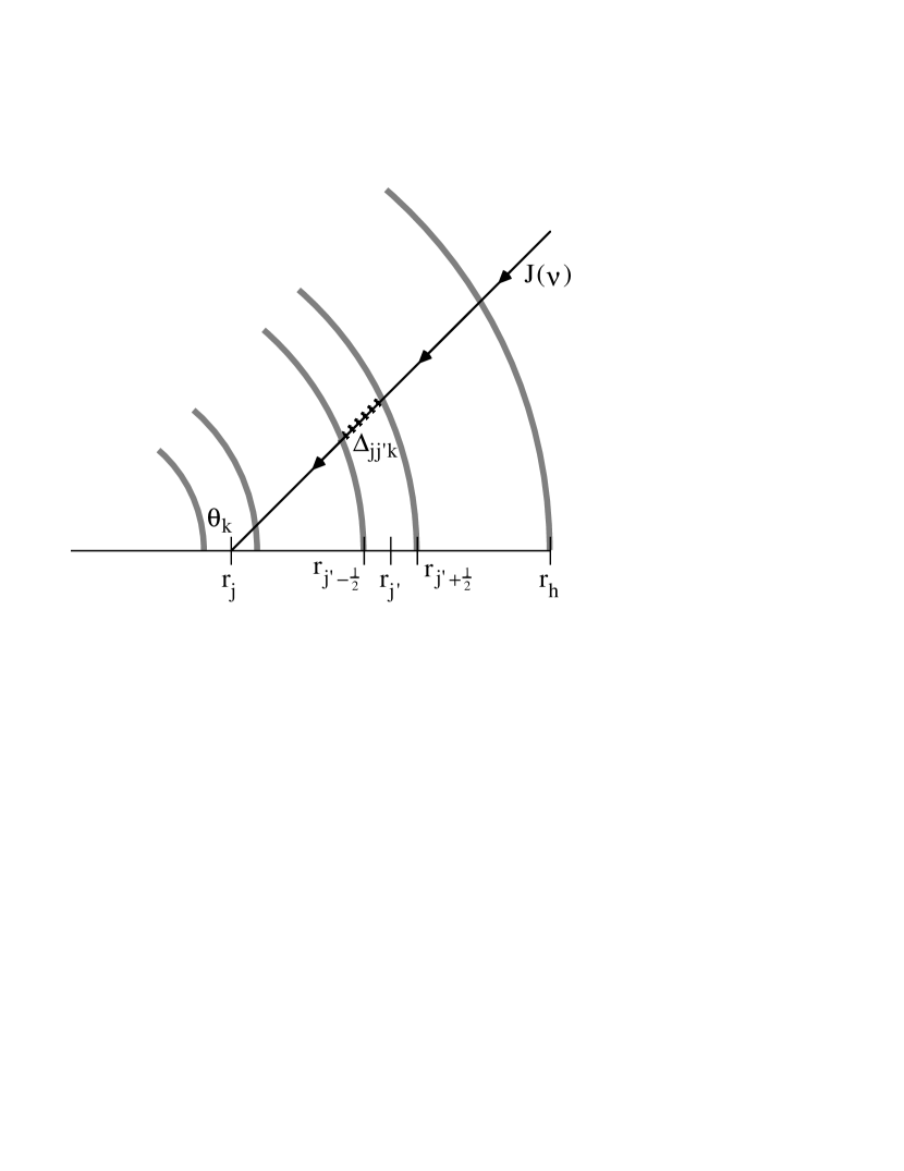
Figure 9: Radiative transfer geometry for an impinging isotropic flux $J(\nu)$. $\Delta_{jj^{\prime}k}$ is the distance traveled through shell $r_{j^{\prime}}$ by an incoming ray bound for shell $r_{j}$ at an angle $\mu_{k}=\cos\theta_{k}$.

References

- Abel et al (1996) Abel, T., Anninos, P., Zhang, Y., & Norman, M.L. 1996, astro-ph/9608040, New Astronomy, submitted
- Anninos et al (1996) Anninos, P., Zhang, Y., Abel, T., & Norman, M.L. 1996, astro-ph/9608041, New Astronomy, submitted
- Babul & Rees (1992) Babul, A., & Rees, M.J. 1992 MNRAS, 255, 346
- Babul & Ferguson (1996) Babul, A., & Ferguson, H.C. 1996, ApJ, 458, 100
- Bechtold et al (1987) Bechtold, J., Weyman, R.J., Lin, Z., & Malkakn, M.A. 1987, ApJ, 315, 180
- Bertschinger (1985) Bertschinger, E. 1985, ApJS, 58, 39
- Bohringer & Hensler (1989) Bohringer, H., & Hensler, G. 1989, å, 215, 147
- Burkert (1995) Burkert, A. 1995, ApJ, 447, L25
- Carignan & Freeman (1988) Carignan, C., & Freeman, K.C. 1988, ApJ, 332, L33
- Dalcanton, Spergel & Summers (1997) Dalcanton, J., Spergel, D., & Summers, F. 1997, ApJ, in press
- Draine & Bertoldi (1996) Draine, B.T., & Bertoldi, F. 1996, ApJ, 468, 269
- de Blok & McGaugh (1996) de Blok, W.J., & McGauh, S. 1996, astro-ph/9610216
- Driver et al (1995) Driver, S.P., et al 1995, ApJ, 453, 48
- Efstathiou (1992) Efstathiou, G. 1992, MNRAS, 256, 43P
- Flores & Primack (1994) Flores, R. & Primack, J.R. 1994, ApJ, 427, 1
- Gunn & Gott (1972) Gunn, J., & Gott, R. 1972, ApJ, 176, 1
- Haiman, Thoul & Loeb (1996) Haiman, Z., Thoul, A., & Loeb, A. 1996, ApJ, 464, 523
- (18) Haiman, Z., Rees, M.J., & Loeb, A. 1996, ApJ, 467, 522
- (19) Haiman, Z., Rees, M.J., & Loeb, A. 1996, astro-ph/9608130, ApJ, submitted
- Haiman & Loeb (1996) Haiman, Z., & Loeb, A. 1996, astro-ph/9611028, ApJ, submitted
- Hoffman (1988) Hoffman, Y. 1996, ApJ, 328, 489
- Ikeuchi (1986) Ikeuchi, S. 1986, Ap&SS, 118, 509
- Ikeuchi, Murakami & Rees (1989) Ikeuchi, S., Murakami, I., & Rees, M.J. 1989, MNRAS, 236, 21P
- Janev (1987) Janev, R.K., Langer, W.D., Evans, Jr. K., & Post, Jr. D.E. 1987, Elementary Processes in Hydrogen-Helium Plasmas (Springer-Verlag)
- Katz, Weinberg & Hernquist (1996) Katz, N., Weinberg, D.H., & Hernquist, L. 1996, ApJS, 105, 19
- Matthews (1972) Matthews, W. 1972, ApJ, 174, 108
- Maloney (1993) Maloney, P. 1993, ApJ, 414, 41
- Moore (1994) Moore, B. 1994, Nature, 370, 629
- Murakami & Ikeuchi (1990) Murakami, I., & Ikeuchi, S. 1990, PASJ, 42, L11
- Navarro & Steinmetz (1996) Navarro, J.F., & Steinmetz, M. 1996, astro-ph/9605043, ApJ, submitted
- Navarro, Frenk & White (1996) Navarro, J.F., Frenk, C.S., & White, S.D.M. 1996, astro-ph/9611107, ApJ, submitted
- Peebles & Dicke (1968) Peebles, J., & Dicke, R. 1968, ApJ, 154, 891
- Rees (1986) Rees, M.J. 1986, MNRAS, 218, 25P
- Shapiro, Grioux & Babul (1994) Shapiro, P.R., Giroux, M.L., & Babul, A. 1994, ApJ, 427, 25
- Shapiro & Kang (1987) Shapiro, P.R., & Kang, H. 1987, ApJ, 318, 32
- Songaila & Cowie (1996) Songaila, A., & Cowie, L. 1996, AJ, 112, 335
- Steidel & Dickinson (1994) Steidel, C., & Dickinson, M. 1994, preprint
- Steidel, Dickinson & Persson (1994) Steidel, C., Dickinson, M., & Persson, E. 1994, ApJ, 437, L75
- Tegmark et al (1996) Tegmark, M., Silk, J., Rees, M.J., Blanchard, A., Abel, T., & Palla, F. 1996, ApJ, 476, ???
- Thoul & Weinberg (1996) Thoule, A., & Weinberg, D.H. 1996, ApJ, 465, 608
- Zhang, Anninos & Norman (1995) Zhang, Y., Anninos, P., & Norman, M.L. 1995, ApJ, 453, L57