ABSTRACT

These lecture notes are organized into ten lessons that summarize the status of inflationary cosmology.

1 Inflation is a Bold and Expansive Paradigm

The hot big-bang cosmology is very successful. It provides a physical description of the Universe from about $10^{-2}\,{\rm sec}$ onward [1]. However, it raises fundamental questions about initial conditions: The origin of the smoothness and flatness of our Hubble volume, the small (one part in $10^{5}$) density inhomogeneities needed to seed all the structure seen in the Universe today, and the tiny baryon asymmetry that results in the existence of matter today.

Inflation explains how a region of size much, much greater than our Hubble volume could have become smooth and flat [2] as well as the origin of the density inhomogeneities needed to seed structure [3]. With regard to the smoothness and flatness, inflation is a temporary fix: It does not guarantee that the observable Universe in the exponentially distant future will be isotropic and homogeneous [4].

Models of inflation are based upon well defined, albeit speculative physics – usually the semi-classical evolution of a weakly coupled scalar field. The physics is speculative because a) there is no evidence for the existence of even a single fundamental scalar field and b) the energy scale associated with inflation is typically much greater than 1 TeV and in most models around $10^{14}\,{\rm GeV}$.

I believe that it is fair to say that inflation has revolutionized the way cosmologists view the Universe. It leads to the current working hypothesis for an extension of the standard cosmology: The Inflation/Cold Dark Matter Paradigm. This paradigm has the potential to extend the standard cosmology back to times as early as $10^{-32}\,{\rm sec}$ and address almost all the pressing questions in cosmology. The key elements of this paradigm are: flat Universe, nonbaryonic dark matter in the form of slowly moving elementary particles (cold dark matter), and nearly scale-invariant, adiabatic density perturbations. As I will emphasize, the inflation/cold dark matter paradigm is highly testable and a flood of observations are doing so. At the outside, within the next decade this paradigm will have been falsified or more firmly established.

There are even grander implications of inflation, albeit very difficult to test [5]. Cosmologists have long used the Copernican principle to argue that the entire Universe must be smooth because of the smoothness of our Hubble volume. In the post-inflation view, our Hubble volume is smooth because it is a small part of a region that underwent inflation, and thus it need not reflect the large-scale features of the Universe as a whole. On the largest scales the structure of the Universe is likely to be very rich: Different regions may have undergone different amounts of inflation, beginning at different times; some regions may not have undergo inflation and may have collapsed to black holes; other regions may be governed by different realizations of the laws of physics because they evolved into different vacuum states of equivalent energy. It is likely that most of the volume of the Universe is still undergoing inflation and that inflationary patches are being constantly produced (eternal inflation). In this case, “the age of the Universe” is a meaningless concept: Our expansion age merely measures the time back to the end of our inflationary event.

If inflation is correct, it will be a major advance in our understanding of the origin and evolution of our Hubble volume and it will open a new window on physics beyond the standard model of particle physics. It is possible that inflation is just plain wrong, and over the years other explanations have put forth to address the dilemma of the initial data. For example, Penrose has suggested the smoothness and flatness of the Universe has to do with the nature of initial singularities [6]. It has, however, been shown that any microphysical solution to the horizon and flatness problems must involve the two key elements of inflation – superluminal expansion and entropy production – suggesting to me that inflation or something closely related is likely to be the correct explanation [7].

2 There is No Standard Model of Inflation

It would be nice if there were a standard model of inflation, but there isn’t. Because inflation involves physics beyond the standard model of particle physics and is probably to tied to fundamental physics at energies of ${\cal O}(10^{14}\,{\rm GeV})$ this is not surprising. What is important, is that inflationary models make three robust predictions (see next Section) which allow the paradigm to be decisively tested. Moreover, cosmological measurements should also be able to discriminate between different models (see final Section).

The two required elements of any inflationary model are: superluminal expansion (i.e., accelerated expansion, $\ddot{R}>0$) and massive entropy production [7]. They are usually achieved by means of the classical evolution of a scalar field rolling down its potential-energy curve. During the first part of its evolution, the field rolls so slowly that its potential energy density is nearly constant; this drives a nearly exponential expansion (superluminal expansion). During the late part of its evolution, the scalar field rapidly oscillates about the minimum of its potential and the decay of these oscillations eventually leads to the production of particles and the reheating of the Universe (entropy production). The entropy produced is the heat that today is the Cosmic Background Radiation (CBR). Because of the massive entropy produced, any initial baryon asymmetry is diluted to a level much, much less than the observed ${\cal O}(10^{-10})$ baryon number per photon and baryogenesis after inflationary is mandatory. The basic mechanics of inflation are well understood and summarized in Ref. [8].

All models of inflation have one feature in common: the scalar field responsible for inflation has a very flat potential-energy curve and is very weakly coupled. This typically implies a dimensionless coupling of the order of $10^{-14}$. Such a small number, like other small numbers in physics (e.g., the ratio of the weak to Planck scales $\approx 10^{-17}$ or the ratio of the mass of the electron to the $W/Z$ boson masses $\approx 10^{-5}$), runs counter to one’s belief that a truly fundamental theory should have no tiny parameters, and cries out for an explanation. In some models, the small number in the inflationary potential is related to other small numbers in particle physics: for example, the ratio of the electron mass to the weak scale or the ratio of the unification scale to the Planck scale. Explaining the origin of the small number associated with inflation is both a challenge and an opportunity.

Models of inflation range from the very simple (e.g., chaotic inflation [9]) to those that attempt to be part of a grander scheme (e.g., models that make contact with speculations about physics at very high energies – grand unification [10], supersymmetry [11, 12, 13], preonic physics [14], or supergravity [15].) Some have attempted to link inflation with superstring theory [16]; others have focussed on the naturalness issue, trying to explain the small dimensionless number associated with inflation [17].

While the scale of the vacuum energy that drives inflation is typically of the order of $(10^{14}\,{\rm GeV})^{4}$, a model of inflation at the electroweak scale, vacuum energy $\approx(1\,{\rm TeV})^{4}$, has been proposed [18]. Multiple epochs of inflation are also possible [19]. Inflation has been considered in the context of alternative theories of gravity. The most successful is first-order inflation [20, 21], where gravity is described by Jordan – Brans – Dicke theory (or a similar theory of gravity) and inflation is triggered by a strongly first-order phase transition (e.g., GUT symmetry breaking) of the kind originally envisioned by Guth [2].

There are certainly details of inflation that are both model-dependent and not completely understood. For example, the basics of reheating were laid out early on [22]; however, important details are still under study today [23]. While the physics issues such as reheating and model building are important and interesting, they do not affect the basic predictions of inflation that are crucial to its testing. In the end, observations may give the best guidance about models and even physics issues.

3 Inflation Makes Three Robust Predictions

Inflation theorists are very inventive and there are probably no set of predictions that are common to all models of inflation. However, a theory without definite predictions is not testable – and is hardly a theory at all (Mach’s principle provides an interesting case in point). The philosopher of science Karl Popper argued that the status of a scientific theory is tied to its vulnerability – strong theories constantly subject themselves to falsification. I believe that inflation is a strong theory in the sense of Popper and that it makes three predictions which allow it to be falsified. They are:

1. Flat universe. This is perhaps the most fundamental prediction of inflation. Through the Friedmann equation it implies that the total energy density is always equal to the critical energy density; it does not however predict the form (or forms) that the critical density takes on today or at any earlier or later epoch.

2. Nearly scale-invariant spectrum of gaussian density perturbations. These density perturbations (scalar metric perturbations) arise from quantum-mechanical fluctuations in the field that drives inflation [3]; they begin on very tiny scales (of the order of $10^{-23}\,$cm) and are stretched to astrophysical size by the tremendous growth of the scale factor during inflation (factor of $e^{60}$ or greater). Scale invariant refers to the fact that the fluctuations in the gravitational potential are independent of length scale; or equivalently that the horizon-crossing amplitudes of the density perturbations are independent of length scale. While the shape of the spectrum of density perturbations is common to all models, the overall amplitude is model dependent. Achieving density perturbations that are consistent with the observed anisotropy of the CBR and large enough to produce the structure seen in the Universe today requires a horizon crossing amplitude of around $(\delta\rho/\rho)_{H}\approx 2\times 10^{-5}$. This is the most severe constraint on inflationary models and leads to the small dimensionless number associated with inflation.

3. Nearly scale-invariant spectrum of gravitational waves. These gravitational waves (tensor metric perturbations) arise during inflation from quantum-mechanical fluctuations in the metric itself and today have wavelengths from ${\cal O}(1\,{\rm km})$ to the size of the present Hubble radius and beyond [24]. Scale invariant here refers to the fact that gravitational waves of all wavelength cross the horizon with the same dimensionless strain amplitude. Once again, the overall amplitude is model dependent (proportional to the inflationary vacuum energy). The uniformity of the CBR provides a cosmological upper bound to the overall amplitude, but unlike density perturbations, there is no cosmological lower bound to the amplitude of gravity-wave perturbations.

There are other interesting consequences of inflation that are not generic. For example, in models of first-order inflation, where reheating occurs through the nucleation and collision of vacuum bubbles, there is an additional, much larger amplitude, but narrow-frequency-band spectrum of gravitational waves ($\Omega_{\rm GW}h^{2}\sim 10^{-7}$) [25]. Large-scale primeval magnetic fields of interesting size can be seeded during inflation [26]. It is also possible to produce topological defects during or near the end of inflation [27] or isocurvature perturbations in a matter component (axions [28], baryons [29], or something else [30]). Such auxiliary predictions are interesting, but are not part of the core predictions that can be used to falsify inflation. On the other hand, they could prove very helpful in establishing inflation.

4 Can Inflation Lead to an Open Universe?

Yes, BUT!!

Whether or not flatness is a generic prediction of inflation has been the topic of much debate recently. I believe that flatness should be taken as a firm prediction of inflation and I will explain why. If there is one episode of inflation, solving the “horizon” problem and solving the “flatness” problem (maintaining $\Omega$ very close to unity until the present epoch) are linked geometrically by the simple expression [31]

$$|\Omega_{0}-1|\mathrel{\mathchoice{\lower 3.6pt\vbox{\halign{$\mathsurround=0pt\displaystyle\hfil#\hfil$\cr<\crcr\sim\crcr}}}{\lower 3.6pt\vbox{\halign{$\mathsurround=0pt\textstyle\hfil#\hfil$\cr<\crcr\sim\crcr}}}{\lower 3.6pt\vbox{\halign{$\mathsurround=0pt\scriptstyle\hfil#\hfil$\cr<\crcr\sim\crcr}}}{\lower 3.6pt\vbox{\halign{$\mathsurround=0pt\scriptscriptstyle\hfil#\hfil$\cr<\crcr\sim\crcr}}}}\left({H_{0}^{-1}\over d_{\rm Patch}}\right)^{2}$$ (1)

where $d_{\rm Patch}$ is the present size of the inflationary patch that our Hubble volume resides within, which is assumed to have size $H^{-1}$ at the beginning of inflation. If we make no assumption about the smoothness of the Universe on superHubble scales before inflation or about our location within our inflationary region, solving the horizon problem requires $H_{0}^{-1}\ll d_{\rm Patch}$ and this implies $|\Omega_{0}-|\ll 1$.

Open inflation requires that this linkage be evaded and that the amount of inflation be tuned to a specific value. The number of e-folds of inflation $N$ is determined by the shape of the scalar-field potential,

$$N={8\pi\over{m_{\rm Pl}}^{2}}\int_{\phi_{i}}^{\phi_{f}}{V(\phi)d\phi\over V^{\prime}}\,.$$ (2)

The value of $N$ required to achieve a given value of $\Omega$ today depends upon the reheating temperature after inflation, the value of $\Omega$ before inflation, and the temperature today,

$$N={1\over 2}\ln\left[{|\Omega_{i}-1|\over|\Omega_{0}-1|}\right]+\ln\left[{T_{\rm RH}T_{0}\over{m_{\rm Pl}}H_{0}}\right]\,.$$ (3)

The amount of inflation needed is linked to both the initial state and the epoch of our existence and invites one to invoke the anthropic principle. I see this as a major step backward and counter to the spirit of the inflationary program.

In any case, the simplest way to evade Eq. (1) is to assume that the smooth patch that inflates has an initial size that is ten or even hundred times larger than the Hubble radius. The more elegant way is to assume two epochs of inflation, the first ending with the nucleation of a bubble and second tied to the slow roll of a scalar field [32]. The open Universe resides within the bubble nucleated by the first episode of inflation (which looks like an open universe [33]) and is reheated by the second, slow-roll epoch of inflation.

Open, double inflation in the context of eternal inflation can trade tuning for a distribution of values of $\Omega_{0}$. My hunch is that the distribution is likely to be very strongly peaked, either around $\Omega_{0}=0$ or $\Omega_{0}=1$, rather than uniform. The recent work of Vilenkin and Winitzki suggests that this is the case [34].

The scientific question of the flatness of the Universe will be answered, probably within the next five years by using the fine-scale anisotropy of the CBR. If the Universe is found to be flat, I will score it as an important victory for inflation. If the flatness prediction is falsified I will consider it a major defeat. If the Universe is found not to be flat, but other tests of inflation prove successful (e.g., CBR anisotropy and/or gravitational waves), I will be willing to take another look at open inflation.

5 Inflation Implies Particle Dark Matter and Maybe More

While inflation predicts a flat, critical-density Universe, it sheds no light on the form that the critical density should take. Cosmological observations have narrowed the possibilities. Denote the fraction of critical density contributed of all forms of energy density by $\Omega_{0}$; inflation predicts $\Omega_{0}=1$. Big-bang nucleosynthesis constrains the baryon density to be well below the critical density: $0.007h^{-2}\leq\Omega_{B}\leq 0.024h^{-2}<0.10$ (for $h>0.5$) [35], which implies that most of the critical density must be in a form other than baryons. When the primeval deuterium abundance is pinned down by a definitive determinations of D/H in high-redshift hydrogen clouds, the baryon density will be pegged to a precision of around 10% or so. Tytler and his collaborators have made a very strong case for a primeval deuterium abundance of D/H$\,\simeq 2.5\times 10^{-5}$ [36], which implies that $\Omega_{B}h^{2}\simeq 0.024$ or $\Omega_{B}\simeq 0.05(0.7/h)^{2}$.

It is also known that: most of the matter is dark (luminous matter contributes less than 1% of the critical density, $\Omega_{\rm LUM}\simeq 0.003h^{-1}$) and the fraction of critical density in matter that clusters exceeds 30%, $\Omega_{M}>0.3$ [37]. Thus, it follows that at least 25% of the critical density should be in the form of nonbaryonic matter in the form of particles, $\Omega_{\rm nbparticles}=\Omega_{M}-\Omega_{B}\mathrel{\mathchoice{\lower 3.6pt\vbox{\halign{$\mathsurround=0pt\displaystyle\hfil#\hfil$\cr>\crcr\sim\crcr}}}{\lower 3.6pt\vbox{\halign{$\mathsurround=0pt\textstyle\hfil#\hfil$\cr>\crcr\sim\crcr}}}{\lower 3.6pt\vbox{\halign{$\mathsurround=0pt\scriptstyle\hfil#\hfil$\cr>\crcr\sim\crcr}}}{\lower 3.6pt\vbox{\halign{$\mathsurround=0pt\scriptscriptstyle\hfil#\hfil$\cr>\crcr\sim\crcr}}}}0.25$. Particle physics has provided three very good candidates whose relic abundance (if they exist) should be of the order of the critical density: an axion of mass around $10^{-5}\,$eV [38]; a neutralino of mass between 10 GeV and 500 GeV [39]; and a neutrino of mass of the order of 10 eV [40].

All are well motivated: the axion is a prediction of the most promising solution to the strong-CP problem; the neutralino is predicted by supersymmetric extensions of the standard model; and essentially all attempts to unify the forces and particles of Nature lead to the prediction that neutrinos have small, but nonzero, masses. In fact, these three particle dark matter candidates are so well motivated that we should probably take seriously the possibility that more than one might contribute significantly to the matter density today.

Finally, it is possible that there is another, even more exotic component, which is smoothly distributed and contributes up to 70% of the critical density, $\Omega_{X}=\Omega_{0}-\Omega_{M}\mathrel{\mathchoice{\lower 3.6pt\vbox{\halign{$\mathsurround=0pt\displaystyle\hfil#\hfil$\cr<\crcr\sim\crcr}}}{\lower 3.6pt\vbox{\halign{$\mathsurround=0pt\textstyle\hfil#\hfil$\cr<\crcr\sim\crcr}}}{\lower 3.6pt\vbox{\halign{$\mathsurround=0pt\scriptstyle\hfil#\hfil$\cr<\crcr\sim\crcr}}}{\lower 3.6pt\vbox{\halign{$\mathsurround=0pt\scriptscriptstyle\hfil#\hfil$\cr<\crcr\sim\crcr}}}}0.7$. The fact that evidence for $\Omega_{M}\sim 1$ is still lacking and that a case is mounting for $\Omega_{M}\sim 0.3$ [37], suggests that inflationists should consider the possibility of a smooth component seriously. Candidates for such include vacuum energy, tangled strings, and rolling scalar fields [41].

While Occam’s Razor argues against a smorgasbord, Nature might enjoy a more interesting meal, and inflation gives no guidance.

6 Large-scale Structure from Quantum Fluctuations

This is perhaps the most striking prediction of inflation, and I believe, the motivation for Stephen Hawking’s description of the COBE DMR discovery of CBR anisotropy [42] as “the most important discovery of all time.” I believe Hawking said this thinking the COBE discovery might prove to be the first evidence that the density perturbations that seeded all structure in the Universe arose from quantum fluctuations during inflation.

Recall, scale invariant refers to density perturbations that cross the horizon with the same amplitude, independent of length scale. Different scales cross the horizon at different times, so the spectrum of density perturbations today is not independent of scale.

Gaussian means that the density contrast, $\delta\rho({\bf x},\,t)/{\bar{\rho}}$, is a gaussian random field, described fully by its two-point correlation function, or equivalently by the power spectrum, which is the Fourier transform of the correlation function and the square of the Fourier transform of the density contrast.

Both scale invariant and gaussian are generic predictions as they are linked to central features of inflation. Because the scalar field that drives inflation is very weakly coupled, it behaves like a free field and its fluctuations are gaussian [3]. The density perturbations are proportional to the scalar-field fluctuations and hence they too should be gaussian. The deviation of the fluctuations from scale invariance is related to the steepness of the scalar potential; since the scalar field responsible for inflation must take the 60 or so Hubble times to evolve to the minimum of its potential in order to solve the horizon/flatness problems its potential cannot be too steep.

The relationship between the inflationary potential and the power spectrum of density perturbations today ($P(k)\equiv\langle|\delta_{k}|^{2}\rangle$) is given by

$$P(k) = {1024\pi^{3}\over 75}\,{k\over H_{0}^{4}}\,{V_{*}^{3}\over{m_{\rm Pl}}^{6}{V_{*}^{\prime}}^{2}}\left(k\over k_{*}\right)^{n-1}T^{2}(k)$$

$$n-1 = -{1\over 8\pi}\left({{m_{\rm Pl}}V^{\prime}_{*}\over V_{*}}\right)^{2}+{{m_{\rm Pl}}\over 4\pi}\left({{m_{\rm Pl}}V_{*}^{\prime}\over V_{*}}\right)^{\prime}$$

$${dn\over d\ln k} = -{1\over 32\pi^{2}}\left({{m_{\rm Pl}}^{3}V_{*}^{\prime\prime\prime}\over V_{*}}\right)\left({{m_{\rm Pl}}V_{*}^{\prime}\over V_{*}}\right)$$

$$\hskip 28.45274pt+{1\over 8\pi^{2}}\left({{m_{\rm Pl}}^{2}V_{*}^{\prime\prime}\over V_{*}}\right)\left({{m_{\rm Pl}}V_{*}^{\prime}\over V_{*}}\right)^{2}-{3\over 32\pi^{2}}\left({m_{\rm Pl}}{V_{*}^{\prime}\over V_{*}}\right)^{4}$$

$$T(q) = {\ln\left(1+2.34q\right)/2.34q\over\left[1+3.89q+(16.1q)^{2}+(5.46q)^{3}+(6.71q)^{4}\right]^{1/4}}\,,$$ (4)

where $V(\phi)$ is the inflationary potential, prime denotes $d/d\phi$, $V_{*}$ is the value of the scalar potential when the scale $k_{*}$ crossed outside the horizon during inflation, $T(k)$ is the transfer function which accounts for the evolution of the mode $k$ from horizon crossing until the present, $q=k/h\Gamma$, and $\Gamma\simeq\Omega_{M}h$ is the “shape” parameter [43]. It is very convenient to chose $k_{*}=H_{0}$ so that $V_{*}$ is the value of the inflationary potential when the scale that fixes the CBR quadrupole crossed outside the horizon. These expressions are given to lowest-order in the deviation from scale invariance, and assume a matter-dominated Universe today; the next-order corrections are given in Ref. [44] and the analogous expressions which include the possibility of a cosmological constant are given in Ref. [45].

Figure 1: Angular power spectra ($C_{l}\equiv\langle|a_{lm}|^{2}\rangle$) of CBR anisotropy for gravity waves (lower curves) and density perturbations (upper curves), normalized to the quadrupole anisotropy; broken lines indicate sampling variance. Temperature fluctuations measured on angular scale $\theta$ are approximately, $(\delta T/T)_{\theta}\sim\sqrt{l(l+1)C_{l}/2\pi}$ with $l\sim 200^{\circ}/\theta$ (courtesy of M. White and U. Seljak).

There are several important things to take note of:

1. The overall amplitude of the power spectrum depends upon the combination $V_{*}^{3}/{V_{*}^{\prime}}^{2}$.

2. The quantity $n-1$, which measures the deviation from scale invariance, is generally not equal to zero [46].

3. The deviation from scale invariance depends upon the steepness of the potential (${m_{\rm Pl}}V_{*}^{\prime}/V_{*}$) and the change in the steepness [47, 89].

4. Typically $n$ is less than 1, and for many models is in the range $0.94$ to $0.96$ [47] (e.g., chaotic inflation [9] and new inflation [49]).

5. There are inflationary models where $n$ is as larger than 1 (e.g., hybrid inflation [50]) and as small as 0.7 (e.g., power-law inflation and natural inflation).

6. Generally, the spectrum of perturbations is nearly, but not exactly, a power law: $dn/d\ln k$ is typically of the order of $-10^{-3}$; only for power-law inflation is the spectrum an exact power law [51].

7. The shape of the transfer function, which determines the level of inhomogeneity on small scales when the power spectrum on large scales is normalized by COBE, depends upon $\Gamma=\Omega_{M}h$ (and to a lesser extent upon the baryon density [52]).

Density perturbations give rise to CBR anisotropy which can be computed very precisely [53]. CBR anisotropy probes the power spectrum at early times ($z\simeq 1100$), when the perturbations were still in the linear regime and astrophysical effects were minimal. Thus, it is one of the most important tests and powerful probes of inflation. Expanding the CBR temperature on the sky in spherical harmonics,

$${\delta T(\theta,\phi)\over T}=\sum_{lm}a_{lm}Y_{lm}(\theta,\phi),$$ (5)

the anisotropy is fully characterized by its angular power spectrum $C_{l}\equiv\langle|a_{lm}|^{2}\rangle$, shown in Fig. 1. The ensemble average for the variance of the multipoles, $\langle|a_{lm}|^{2}\rangle$, is related to the power spectrum (as described in Ref. [53]); note, isotropy in the mean implies $\langle a_{lm}\rangle=0$. The variance of multipole $l$ is dominated by modes of wavenumbers $k\simeq lH_{0}/2$. CBR anisotropy on large-angular scales ($l\ll 100$) arises almost solely from the Sachs-Wolfe effect and to good approximation can be computed analytically [8, 54]

$$C_{l}={H_{0}^{4}\over 2\pi}\int_{0}^{\infty}(u/u_{\rm EQ})|j_{l}(u)|^{2}P(u/u_{\rm EQ})du/u\,,$$ (6)

where $u=k\tau_{0}$ and $u_{\rm EQ}=k_{\rm EQ}\tau_{0}$. The variance of the quadrupole anisotropy provides a handy means of normalizing the power spectrum

$$S\equiv{5\langle|a_{2m}|^{2}\rangle\over 4\pi}\simeq 2.2\,{V_{*}/m_{\rm Pl}^{4}\over(m_{\rm Pl}V_{*}^{\prime}/V_{*})^{2}}.$$ (7)

The detection of CBR anisotropy by the COBE DMR was a major advance as it allowed the spectrum of density perturbations to be normalized on very large scales ($k\sim H_{0}$). For precisely scale-invariant density perturbations and no gravitational-wave contribution to CBR anisotropy the normalization procedure is easy to describe: $S$ is equated to the COBE determination of the variance of the quadrupole anisotropy, $Q_{\rm COBE}=(17\mu\,{\rm K}/2.2728\,{\rm K})^{2}\simeq 3.8\times 10^{-11}$ [55], which then implies

$${V_{*}/m_{\rm Pl}^{4}\over(m_{\rm Pl}V_{*}^{\prime}/V_{*})^{2}}=1.8\times 10^{-11}$$ (8)

Bunn et al. [56] have done a careful analysis of the COBE four-year data which takes account of the fact that the COBE normalization for $S$ depends upon $n$ as well as the possible contribution of gravitational waves to CBR anisotropy. (The “pivot point” for the COBE data is $l\sim 15$; that is, the COBE determinations of $C_{15}$ and $n$ are almost uncorrelated.) This leads to the more accurate normalization

$${V_{*}/m_{\rm Pl}^{4}\over(m_{\rm Pl}V_{*}^{\prime}/V_{*})^{2}}=1.7\times 10^{-11}\,{\exp[-2.02(n-1)]\over\sqrt{1+{2\over 3}{T\over S}}}$$ (9)

where $T$ is the tensor contribution to the variance of the CBR quadrupole. The $1\sigma$ error is 15%. (Bunn et al. have also generalized this result to allow for the possibility of a cosmological constant [56].)

The Bunn et al. normalization can also be expressed in terms of the horizon-crossing amplitude for the comoving scale $k=H_{0}$:

$$\delta_{H}(k=H_{0})\equiv\left[{k^{3/2}|\delta_{k}|\over\sqrt{2\pi^{2}}}\right]_{k=H_{0}}=1.9\times 10^{-5}\,{\exp[-1.01(n-1)]\over\sqrt{1+{2\over 3}\,{T\over S}}}.$$ (10)

7 Gravitational Waves: The Smokin’ Gun

The inflation-produced gravitational waves are the smokin’ gun signature of inflation and crucial to learning about the inflationary potential. Both a flat Universe [57] and scale-invariant density perturbations (so called Harrison–Zel’dovich spectrum [58]) were discussed as features of any “sensible cosmology” long before inflation. The nearly scale-invariant spectrum of gravitational waves which arises from quantum mechanical fluctuations excited in the space-time metric during inflation is a very important prediction of inflation that sets it apart from just any other sensible cosmology. Detecting these gravitational waves will be very challenging.

Unlike the scalar perturbations, which must have an amplitude of around $10^{-5}$ to seed structure formation, there is no astrophysical clue as to the amplitude of the tensor perturbations. They can be characterized by their power spectrum today [59]

$$P_{T}(k) \equiv \langle|h_{k}|^{2}\rangle={8\over 3\pi}{V_{*}\over{m_{\rm Pl}}^{4}}\left(k\over k_{*}\right)^{n_{T}-3}T_{T}^{2}(k)$$

$$n_{T} = -{1\over 8\pi}\left({{m_{\rm Pl}}V^{\prime}_{*}\over V_{*}}\right)^{2}$$

$${dn_{T}\over d\ln k} = {1\over 32\pi^{2}}\left({{m_{\rm Pl}}^{2}V^{\prime\prime}\over V}\right)\left({{m_{\rm Pl}}V^{\prime}\over V}\right)^{2}-{1\over 32\pi^{2}}\left({{m_{\rm Pl}}V^{\prime}\over V}\right)^{4}=-n_{T}[(n-1)-n_{T}]$$

$$T_{T}(k) \simeq \left[1+{4\over 3}{k\over k_{\rm EQ}}+{5\over 2}\left({k\over k_{\rm EQ}}\right)^{2}\right]^{1/2},$$ (11)

where $T_{T}(k)$ is the transfer function for gravity waves and describes the evolution of mode $k$ from horizon crossing until the present, $k_{\rm EQ}=6.22\times 10^{-2}\,{\rm Mpc^{-1}}\,(\Omega_{M}h^{2}/\sqrt{g_{*}/3.36})$ is the scale that crossed the horizon at matter-radiation equality, $\Omega_{M}$ is the fraction of critical density in matter, and $g_{*}$ counts the effective number of relativistic degrees of freedom (3.36 for photons and three light neutrino species). The quantity $k^{3/2}|h_{k}|/\sqrt{2\pi^{2}}$ corresponds to the dimensionless strain (metric perturbation) on length scale $\lambda=2\pi/k$.

Like density perturbations, gravity waves lead to CBR anisotropy which can be fully described by an angular power spectrum. The gravity-wave angular power spectrum is related to the power spectrum and can be computed very accurately [60]; it is shown in Fig. 1. The following analytical expression is accurate to about 10%,

$$C_{l} = 36\pi^{2}{\Gamma(l+3)\over\Gamma(l-1)}\,\int_{0}^{\infty}\,F_{l}(u)(u/u_{\rm EQ})^{3}P_{T}(u/u_{\rm EQ})\,du/u$$

$$F_{l}(u) = -\int^{u}_{(\tau_{\rm LS}/\tau_{0})u}dy\left({j_{2}(y)\over y}\right)\left({j_{l}(u-y)\over(u-y)^{2}}\right)$$ (12)

where $u=k\tau_{0}$, $\tau_{0}=2H_{0}^{-1}$ is the conformal age of the Universe today, and $\tau_{\rm LS}=\tau_{0}/\sqrt{(1+z_{\rm LS})}$ is the conformal age at last scattering. The tensor contribution to the variance of the CBR quadrupole is a convenient normalization for the spectrum:

$$T\equiv{5\langle|a_{2m}|^{2}\rangle\over 4\pi}=0.61(V_{*}/m_{\rm Pl}^{4}).$$ (14)

The predicted variance of the CBR quadrupole anisotropy is $T+S$.

Figure 2: Polarization angular power spectra for gravity waves (broken) and density perturbations (solid). The polarization of the CBR anisotropy is roughly $\sqrt{C_{l}^{P}/C_{l}}$ (courtesy of M. White and U. Seljak).

There are several important things to take note of:

1. The contribution of gravity waves to the variance of the CBR quadrupole is proportional to the value of the vacuum energy that drives inflation, and if $T$ can be determined, the energy scale of inflation can be determined.

2. Using the COBE four-year results as an upper bound, $T<Q_{\rm COBE}$, it follows that, $V_{*}<6\times 10^{-11}{m_{\rm Pl}}^{4}$, or equivalently, $V_{*}^{1/4}<3.4\times 10^{16}\,{\rm GeV}$. This indicates that inflation, if it occurred, involved energies much smaller than the Planck scale. (To be more precise, inflation could have begun at a much higher energy scale, but the portion of inflation relevant for us, i.e., the last 60 or so e-folds, occurred at an energy scale much smaller than the Planck energy. In chaotic inflation [9], inflation is supposed to begin at the Planck energy density.)

3. The four potential observables, $S$, $T$, $n-1$ and $n_{T}$, depend upon three properties of the inflationary potential, $V_{*}$, $V_{*}^{\prime}$ and $V_{*}^{\prime\prime}$. Thus, the potential and its first two derivatives can be expressed in terms of the four observables with an additional consistency relation, $T/S=-7n_{T}$, which is an important test of inflation [61]. If $S$, $T$, and $n-1$ can be determined, the potential and its first two derivatives can be “reconstructed”; in addition, if $n_{T}$ can also be measured, the consistency of inflation can be tested [62].

4. The amplitude of the gravity-wave spectrum and its “tilt” (deviation from scale invariance) are related: the larger the amplitude, the greater the tilt. Moreover, this means the spectrum of gravity waves can be described by a single parameter.

5. The tensor tilt, deviation of $n_{T}$ from 0, and the scalar tilt, deviation of $n-1$ from zero, are in general not equal; they differ by the rate of change of the steepness. The only model where they are identical is power-law inflation.

6. The variation of the tensor index with scale, $dn_{T}/d\ln k$, is typically ${\cal O}(10^{-3})$.

There are two basic approaches to detecting the tensor perturbations: CBR anisotropy and/or polarization and direct detection of gravity waves. The first approach probes the spectrum at very long wavelengths, $\lambda\sim H_{0}^{-1}/100-H_{0}^{-1}\sim 10^{26}\,{\rm cm}-10^{28}\,{\rm cm}$, while the second probes much shorter wavelengths, $\lambda\sim 10^{8}\,{\rm cm}-10^{14}\,{\rm cm}$. If some information (detections/upper limits) could be obtained at both wavelengths, both $T$ and $n_{T}$ could be measured or at least constrained.

While the scalar and tensor angular power spectra are very different (see Fig. 1), sampling variance sets a fundamental limit to how well the two can be separated from measurements of the one CBR sky we have access to. For multipole $l$, $2l+1$ multipole amplitudes can be used to determine the variance; “the variance of the variance” is

$${\langle(C_{l}^{\rm estimate}-C_{l})^{2}\rangle^{1/2}\over C_{l}}=\sqrt{2\over 2l+1},$$ (15)

where $C_{l}^{\rm estimate}$ is the estimate based upon CBR measurements; sampling variance is shown in Fig. 1. Using anisotropy alone, sampling variance implies that the tensor contribution can be reliably separated only if $T/S\geq 0.1$ [63]. The tensor and scalar perturbations led to different levels of polarization of the anisotropy; see Fig. 2. The sampling-variance limit based upon CBR polarization is about a factor of five smaller [63], but requires that polarization on large-angular scales be measured at less than a fraction of a percent. Recently, it has been pointed out that scalar and tensor perturbations excite different patterns of polarization [64], which could allow sampling variance to be evaded. In any case, the potential of polarization remains to be seen: the signal is small (maximum polarization is a few percent of the anisotropy); CBR polarization has yet to be detected; and the severity of polarization foregrounds are yet to be determined.

Earth-based laser interferometers which operate in the 10 Hz to kHz range are being built in the US (LIGO) and in Europe (VIRGO). A space-based interferometer is being planned by ESA (LISA) and ideas for a smaller mission are being discussed in the US (OMEGA). Space-based interferometers could operate at frequencies as low as $10^{-4}\,$Hz.

Figure 3: Spectral energy density in gravity waves produced by inflation; for $T/S=0.018$, $dn_{T}/d\ln k=-10^{-3}$, 0, $10^{-3}$. $T/S=0.18$ (heavy curve) maximizes the energy density at $f=10^{-4}\,$Hz. Curves are from Eq. (16) using $H_{0}=60{\rm km\,s^{-1}\,Mpc^{-1}}$, $\Omega_{M}=1$, and $g_{*}=3.36$ (from Ref. [65]).

It is straightforward to go from the power spectrum to the fraction of critical density contributed by gravity waves per log frequency interval

$$\Omega_{\rm GW}(f)\equiv{1\over\rho_{\rm crit}}\,{d\rho_{\rm GW}\over d\ln k}={\Omega_{M}^{2}\,V_{*}/m_{\rm Pl}^{4}\,\over(k/H_{0})^{2-n_{T}}}\left[1+{4\over 3}{k\over k_{\rm EQ}}+{5\over 2}\left({k\over k_{\rm EQ}}\right)^{2}\right],$$ (16)

where $f=k/2\pi$ and $\Omega_{\rm GW}(f)$ is shown in Fig. 3. The long plateau, frequencies greater than $f_{\rm EQ}=k_{\rm EQ}/2\pi\sim 10^{-15}\,$Hz, reflects the scale invariance of the gravitational-wave spectrum. The rise for smaller frequencies, as $f^{2}$, traces to the fact that the longest wavelength modes crossed the horizon during the matter-dominated epoch. The energy density in gravitational waves can also be expressed in terms of the rms metric perturbation or strain, $h_{rms}^{2}(k)\equiv k^{3}|h_{\bf k}|^{2}/2\pi^{2}$,

$$\Omega_{\rm GW}(f)={2\pi^{2}\over 3}\,\left({f\over H_{0}}\right)^{2}\,h_{rms}^{2}(k)=6.3h^{-2}\times 10^{-7}\,(f/{\rm Hz})^{2}$$ (17)

Using the relationship between the tensor spectral index $n_{T}$ and the amplitude $T$, and the COBE determination of the variance of the CBR quadrupole anisotropy, Eq. (16) can be rewritten in terms of $n_{T}$ (or $T/S$) alone [65]. Doing so, it then follows that on the “long plateau” ($f\gg 10^{-15}\,$Hz)

$$\Omega_{\rm GW}(f)h^{2} = 5.1\times 10^{-15}\,(g_{*}/3.36)\,{n_{T}\over n_{T}-1/7}$$ (18)

$$\times \exp[n_{T}N+{1\over 2}N^{2}(dn_{T}/d\ln k)],$$

where $N\equiv\ln(k/H_{0})\simeq 33+\ln(f/10^{-4}{\rm Hz})+\ln(0.6/h)$ and I have also allowed for the possible variation of the tensor index $n_{T}$ which is typically $-10^{-3}$.

The importance of the amplitude – tilt relationship can be seen in Fig. 3. Sadly, tilt goes in the direction of pushing $\Omega_{\rm GW}$ down as the amplitude $T/S$ is increased. There is a bright side: $\Omega_{\rm GW}(f\sim{\rm Hz})$ is maximized for $T/S\simeq 0.18$, which is close to the value predicted by chaotic inflation and exceeds the sampling-variance limit to the detection of tensor perturbations using CBR anisotropy alone. While there are essentially no inflationary models where $|n-1|\ll 0.1$, there are many models where $-n_{T}\ll 0.1$ (e.g., natural inflation and new inflation). Because of the amplitude – tilt relationship, the gravity-wave background in these models is very small.

The range of $T/S$ accessible to a gravity-wave detector operating at $f=10^{-4}\,$Hz (appropriate for LISA) and $f=100\,$Hz (appropriate for LIGO and VIRGO) is shown as a function of the detector energy sensitivity in Fig. 4 [65]. A sensitivity of $\Omega_{\rm GW}(f)h^{2}\sim 10^{-15}$ is needed for a serious search for inflation-produced gravity waves. With its initial strain detectors, the earth-based LIGO should be able to detect a stochastic background of gravity waves with 90% confidence provided $\Omega_{\rm GW}(f\sim 100\,{\rm Hz})h^{2}\geq 2.8\times 10^{-6}$; with advanced strain detectors this should improve to $2.8\times 10^{-11}$ [66, 67]. Unfortunately, this misses the mark by four orders of magnitude. (If one were to ignore the relation between tilt and amplitude and assume $n_{T}\equiv 0$, LIGO would only miss by three orders of magnitude [67].)

Figure 4: The range of $T/S$ probed (interval interior to parabola) as a function of energy sensitivity for $f=10^{-4}\,$Hz (solid curves) and $f=100\,$Hz (broken curves). The “pessimistic” (left) parabola assumes $dn_{T}/d\ln k=-10^{-3}$ and the “optimistic” (right) parabola assumes $dn_{T}/d\ln k=10^{-3}$. Also shown are the sampling-variance limiting sensitivities for CBR anisotropy and polarization (from Ref. [65]).

Because the energy density in gravity waves is proportional to strain squared times frequency squared, a detector operating at lower frequency has better energy-density sensitivity for fixed strain sensitivity. Earth-based detectors cannot cannot operate at lower frequencies because of seismic noise, but space-based detectors can. The design study for the space-based LISA indicates an energy sensitivity of around $\Omega_{\rm GW}(f)h^{2}\sim 10^{-13}$ at $f=10^{-4}\,$Hz [68], which is more promising, but still misses by two orders of magnitude. (There is also a worrisome background of coalescing white-dwarf binaries, which could dominate inflation at frequencies greater than around $10^{-4}\,$Hz [69].)

Detection of the inflation-produced gravity waves presents a very great challenge. But the possible payoffs are commensurately large: A smokin’ gun test of inflation; a determination of the energy scale of inflation (through $T$); and a consistency test of inflation (through $n_{T}$ and $T/S$).

8 CDM: A Testable, Ten Parameter Theory

CBR anisotropy has been detected on angular scales ranging from $100^{\circ}$ to a fraction of degree at the level of about $\delta T/T\sim 10^{-5}$ (see Fig. 5). This provides strong support for the notion that structure formed by the gravitational amplification of small primeval density inhomogeneities. One of the pressing problems in cosmology is the formulation of a detailed and coherent picture of structure formation. The two key elements in any such theory are the quantity and composition of matter in the Universe and the nature of the perturbations that seed the formation of structure. Inflation makes definite predictions about both, and with the rapidly growing number of high-quality observations that bear on the issue, structure formation has become an important testing ground for inflation.

Recall, inflation and astrophysical data indicate the following about the quantity and composition of matter in the Universe: baryons contribute a small fraction of the critical density, $\Omega_{B}=(0.007-0.024)h^{-2}$; particle dark matter plus baryons contribute at least 30% of the critical density; and there may be a smooth component that brings the total to the critical density. The inflationary prediction concerning the seed perturbations is sharper: almost scale-invariant gaussian density perturbations, whose horizon-crossing amplitude is determined by COBE to be about $2\times 10^{-5}$.

Particle dark matter can be classified by its velocity dispersion at the epoch of matter – radiation equality: cold, $v_{rms}\ll 1$; hot, $v_{rms}\sim 1$; and warm, $v_{rms}$ not too much smaller than 1. Neutrinos and neutralinos were once in thermal equilibrium and their velocity dispersion is set by the temperature at matter – radiation equality ($T_{\rm EQ}\simeq 6h^{2}{\,\rm eV}$) and is inversely proportional to their mass. Neutrinos are light and therefore hot; neutralinos are heavy and therefore cold. Axions are cold in spite of their small mass because they were never in thermal equilibrium and were produced by a coherent, rather than thermal, process [38]. Around the time of matter – radiation equality, density perturbations on small scales can be damped by the freestreaming of dark matter particles from regions of high density to regions of low density; for neutrinos this is a significant effect and perturbations on scales less than about 30 Mpc are strongly damped. For cold dark matter the freestreaming scale is much less than 1 Mpc and most likely uninteresting. For warm dark matter the freestreaming scale is around 1 Mpc (essentially by definition) and has interesting consequences.

Figure 5: Summary of CBR anisotropy measurements and predictions for two CDM models. Plotted are the squares of the measured multipole amplitudes ($C_{l}=\langle|a_{lm}|^{2}\rangle$) versus multipole number $l$. The relative temperature difference on angular scale $\theta$ is given roughly by $\sqrt{l(l+1)C_{l}/2\pi}$ with $l\sim 200^{\circ}/\theta$. The theoretical curves are standard CDM (upper curve) and CDM with $n=0.7$ and $h=0.5$ (lower curve) (from Ref. [74]).

For hot dark matter structure must form “top down” – superclusters form and fragment into galaxies. More than a decade ago this possibility was studied and was found to be wanting [70]. Put simply, there is every evidence that structure formed from the bottom up: The bulk of the galaxies formed at redshifts from two to four and superclusters are only forming today. Warm dark matter is problematic because subgalactic-sized objects must form from the fragmentation of galaxies; the abundance of high-redshift (up to redshifts of almost five) hydrogen clouds is difficult at best to reconcile with this fact [71]. That leaves cold dark matter as the unique “prediction” of inflation. As we shall see, this prediction has been very successful.

Here are the essential features of CDM [72, 73]: (1) it is hierarchical, with smaller things forming first and larger things forming (slightly) later; (2) because the amplitude of density perturbations on very small scales varies slowly with scale, $k^{2/3}|\delta_{k}|\propto\log k$ for $k\gg k_{\rm EQ}$, structure formation is not strongly hierarchical; (3) in COBE normalized CDM the first stars (in globular-cluster size objects) form at redshifts of ten or so, galaxies begin forming at redshifts of five (with the bulk forming between $z\sim 4$ and $z\sim 2$), clusters begin forming at redshifts around one, and superclusters are just becoming gravitationally bound today; (4) CDM particles form the cosmic infrastructure on all scales – in galaxies they are the dark halos and in clusters they are the dark matter that pervades the cluster.

When the CDM scenario emerged more than a decade ago many referred to it as a no-parameter theory because it was so specific compared to previous models for the formation of structure. This was an overstatement as there are cosmological quantities that must be specified. However, the data available did not require precise knowledge of these quantities to begin testing the CDM paradigm.

Broadly speaking the parameters can be organized into two groups [74]. First are the cosmological parameters: the Hubble constant $h$; the density of ordinary matter, $\Omega_{B}h^{2}$; the amplitude of the scalar perturbations, $S$, the scalar power-law index, $n$, and the rate at which it varies, $dn/d\ln k$; the amplitude of the tensor perturbations, $T/S$, and tensor power-law index, $n_{T}$. The inflationary parameters fall into this category because there is no standard model of inflation; on the other hand, once determined they can be used to discriminate among models of inflation.

The second group specifies the composition of invisible matter in the Universe: radiation, dark matter, and vacuum energy. Radiation refers to relativistic particles: the photons in the CBR, three massless neutrino species (assuming none of the neutrino species has a mass), and possibly other undetected relativistic particles (some particle-physics theories predict the existence of additional massless particle species). At present relativistic particles contribute almost nothing to the energy density in the Universe, $\Omega_{R}\simeq 4.2\times 10^{-5}h^{-2}$; early on – when the Universe was smaller than about $10^{-5}$ of its present size – they dominated the energy content; the level of radiation today is important as it determines when the transition from radiation domination to matter domination took place and thereby the shape of the transfer function (through $\Gamma$).

Dark matter could include other particle relics besides CDM. For example, each neutrino species has a number density of $113{\,{\rm cm}^{-3}}$, and a neutrino species of mass $5{\,\rm eV}$ would account for about 20% of the critical density ($\Omega_{\nu}=m_{\nu}/90h^{2}{\,\rm eV}$). Predictions for neutrino masses range from $10^{-12}{\,\rm eV}$ to several MeV, and there is some experimental evidence that at least one of the neutrino species has a small mass [75]. Finally, there is the cosmological constant. Introduced and then abandoned by Einstein to prevent the expansion of the Universe, and resurrected by Bondi, Gold and Hoyle in 1948 to address an age crisis, it is still with us. In the modern context it corresponds to an energy density associated with the quantum vacuum. At present, there is no reliable calculation of the value that the cosmological constant should take [76], and so its existence must be regarded as a logical possibility, with its value to be determined by observations. (As mentioned earlier, there are even more exotic possibilities for the smooth component [41].)

The original no-parameter CDM model, often referred to as standard CDM [72], is characterized by simple choices for the cosmological and the invisible matter parameters: precisely scale-invariant density perturbations ($n=1$), $h=0.5$, $\Omega_{B}=0.05$, $\Omega_{\rm CDM}=0.95$; no radiation beyond the photons and the three massless neutrinos; no dark matter beyond CDM; and zero cosmological constant. Standard CDM served its purpose well as the DOS 1.0 of cosmology: it focussed attention on a specific CDM model.

While inflation models predict that the shape of the spectrum is approximately scale-invariant, the overall amplitude depends on the particular inflationary model. For standard CDM the overall amplitude was fixed by comparing the predicted level of inhomogeneity with that seen today in the distribution of bright galaxies. Galaxy-number fluctuations in spheres of radius $8h^{-1}\,{\rm Mpc}$ are unity:

$$\sigma_{r}^{2}\equiv\int_{0}^{\infty}{dk\over k}\ {k^{3}P(k)\over 2\pi^{2}}\,\left({3j_{1}(kr)\over kr}\right)^{2}=1$$ (19)

for $r=8\,h^{-1}$Mpc. This normalization ($\sigma_{8}=1$) corresponds to the assumption that light, in the form of bright galaxies, traces mass. Choosing $\sigma_{8}$ to be less than one means that light is more clustered than mass and is a biased tracer of mass. There is some evidence that bright galaxies are somewhat more clumped than mass with biasing factor $b\equiv 1/\sigma_{8}\simeq 1-2$; e.g., the number fluctuations of IRAS galaxies on the $8h^{-1}\,{\rm Mpc}$ scale is less than one:, $\sigma_{8}({\rm IRAS})=0.69\pm 0.04$ [77], implying that infrared selected galaxies are less clustered than optically bright galaxies.

As discussed earlier, COBE changed the normalization procedure; given the values of the CDM parameters and normalizing to COBE $\sigma_{8}$ can be computed. Further, an independent means of determining $\sigma_{8}$, based upon the abundance of rich clusters, has been developed; comparing this value to the that computed from the COBE normalized spectrum now provides a check/constraint. But I am getting ahead of myself.

Is a ten parameter theory testable? With sufficient high-quality data the answer is yes. The standard model of particle physics has at least nineteen parameters; not only has it been tested, but most of the parameters have been determined, many to better than 1% precision. In the next two Sections I hope to make the case that inflation/cold dark matter can be tested with the same decisiveness. Much of my case will rely upon CBR anisotropy; if 2000 or so multipoles can be measured to a precision close to that dictated by sampling variance, I believe this ambitious goal is achievable.

9 Status of Inflation: So Far, So Good

The testing of inflation necessarily focuses on its three robust predictions and their consequences.

9.1 Flatness

The first prediction is a flat Universe with nonbaryonic dark matter. There is strong evidence coming from a number of directions that $\Omega_{M}$ is at least 0.3 [37]. This makes nonbaryonic dark matter inescapable since the big-bang nucleosynthesis upper bound is $\Omega_{B}<0.024h^{-2}<0.10$ (for $h>0.5$) and is half way (on a logarithmic scale) to the simplest realization of a flat Universe, $\Omega_{M}=1$; see Fig. 6. In the case that $\Omega_{M}\approx 0.3$ it is possible that the bulk of the closure density resides in a smooth component.

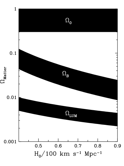
Figure 6: Summary of knowledge of $\Omega_{M}$. The lowest band is luminous matter, in the form of bright stars and associated material; the middle band is the big-bang nucleosynthesis determination of the density of baryons; the upper region is the estimate based upon the peculiar velocities of galaxies and other dynamical methods [37]. The gaps between the bands illustrate the two dark matter problems: most of the ordinary matter is dark and most of the matter is nonbaryonic (from Ref. [74]).

Testing the flatness prediction has an even brighter future. The position of the first acoustic (Doppler) peak is sensitive to $\Omega_{0}$, $l_{\rm peak}\simeq 220/\sqrt{\Omega_{0}}$. The current data, while certainly not definitive, put a smile on my face: Hancock infers $\Omega_{0}=0.7^{+1.0}_{-0.4}$ [78]. It is likely that even before MAP is launched in 2000, ground-based and balloon-based measurements will determine the position of the first acoustic peak well enough to peg $\Omega_{0}$ to 10%.

Measurements of the deceleration of the Universe using the magnitude – redshift diagram for SNeIa constrain a nearly orthogonal combination, $\Omega_{M}-\Omega_{\Lambda}$; together, they can determine both $\Omega_{M}$ and $\Omega_{\Lambda}$. (One should keep in mind that there are more exotic possibilities for the smooth component [41, 80].) Assuming a flat Universe and using their first seven SNeIa, Perlmutter et al [79] derive the bound $\Omega_{\Lambda}<0.51$ (95%); or without the assumption of flatness, $-0.4<\Omega_{M}-\Omega_{\Lambda}<2.7$ (95%). Perlmutter’s group, the Supernova Cosmology Project, now has a total of more than fifty SNeIa at redshifts $z\sim 0.4-0.8$, and the High-Redshift Supernova Team has a similar number; more definitive results should be coming soon.

The combination of the age and Hubble constant can, in principle, determine or at least constrain $\Omega_{M}$ and $\Omega_{\Lambda}$. At the moment, the uncertainties preclude any firm conclusions. Taken at face value, the data seem to favor a cosmological constant (if the Universe is flat); see Fig. 7.

A key consequence of the flatness prediction is the existence of nonbaryonic dark matter. The cold dark matter scenario won’t be fully tested until CDM particles are detected. A large-scale search for halo axions with sufficient sensitivity to detect them (if they are there) is now underway [81], and soon, CDMS, the Stanford – Berkeley – Case Western – UCSB bolometric detector, will began searching for halo neutralinos with sufficient sensitivity to detect them for some models of low-energy supersymmetry [82]. SuperKamiokande and MACRO can search indirectly for neutralinos that annihilate in the sun and produce high-energy neutrinos, and Ting’s AMS, which will be flown on the shuttle a year from now, will be able to search for positrons and antiprotons produced by neutralino annihilations in the halo.

Figure 7: The relationship between age and $H_{0}$ for flat-universe models with $\Omega_{M}=1-\Omega_{\Lambda}$. The cross-hatched region is ruled out because $\Omega_{M}<0.3$. The dotted lines indicate the favored range for $H_{0}$ and for the age of the Universe (based upon the ages of the oldest stars) (from Ref. [74]).

9.2 Gravity waves

The search for inflation-produced gravitational waves was summarized in Section 7.

9.3 Density Perturbations/Cold Dark Matter

Figure 5 summarizes the status of testing the second robust prediction of inflation through CBR anisotropy: The measurements are generally consistent with the inflationary prediction. The power-law index is constrained to be $1.1\pm 0.2$, which is well within the range predicted by inflation, and when COBE is used to normalize the spectrum, there are CDM models that are consistent with all the other observations.

Figure 8: Measurements of the power spectrum, $P(k)=|\delta_{k}|^{2}$, and the predictions of different COBE-normalized CDM models. (COBE constrains the power spectrum at wavenumbers $k$ around $2h\times 10^{-3}\,{\rm Mpc}$ as indicated by rectangle.) The points are from several redshift surveys as compiled by [83]; the models are: $\Lambda$CDM with $\Omega_{\Lambda}=0.6$ and $h=0.65$; standard CDM (sCDM), CDM with $h=0.35$; $\tau$CDM (with the energy equivalent of 12 massless neutrino species) and $\nu$CDM with $\Omega_{\nu}=0.2$ (unspecified parameters have their standard CDM values). The offset between a model and the points indicates the level of biasing. Note, $\Lambda$CDM does not pass through the COBE rectangle because a cosmological constant alters the relation between the power spectrum and CBR anisotropy (from Ref. [74]).

There is much data that can be used to test the cold dark matter scenario. To focus the discussion, I will consider four “families” of models, distinguished by their invisible matter content: standard invisible matter content (CDM); extra radiation ($\tau$CDM); small hot dark matter component ($\nu$CDM); and cosmological constant ($\Lambda$CDM). There are of course other possibilities: extra radiation + cosmological constant, or a more exotic smooth component, which has been analyzed in Ref. [80]. Within each family, the five cosmological parameters ($h$, $\Omega_{B}h^{2}$, $n$, $T/S$ and $n_{T}$) must be specified. Once specified, the power spectrum can be COBE-normalized and the expected level of inhomogeneity in the Universe today computed.

In assessing the viability of CDM models I will summarize work done in collaboration with Dodelson and Gates [74]; others have done similar work [84]. We began with three robust observational constraints on the power spectrum: the shape of the power spectrum; the power on cluster scales; and the early formation of objects. The first constraint, the shape of the power spectrum on scales from a few Mpc to a few 100 Mpc (see Fig. 8), comes from redshift surveys of the distribution of bright galaxies today [83]. In the absence of an understanding of the relationship between the distribution of light, which is what these surveys determine, and of mass, the bias factor is left as a free parameter. Models whose power spectra deviates from the measured power spectrum (as compiled in Ref. [83]) by more than two sigma (value of $\chi^{2}$ whose likelihood is less than 5%) were rejected. (Very roughly, this constrains the shape parameter: $\Gamma=\Omega_{M}h=0.25\pm 0.1$.)

The abundance of x-ray emitting clusters is sensitive to the level of inhomogeneity on scales around $8h^{-1}\,{\rm Mpc}$ and thus provides a good means of inferring the value of $\sigma_{8}$. Following [85] we used $0.5\leq\sigma_{8}\leq 0.8$ for models with $\Omega_{M}=1$ and let this range scale with $\Omega^{-0.56}$ for models with a cosmological constant ($\Omega_{\Lambda}=1-\Omega_{M}$) [86].

The formation of objects at high redshift (early structure formation) probes the power spectrum on small scales. At redshifts of two to four, hydrogen clouds, detected by their absorption features in the spectra of high-redshift quasars ($z\sim 4-5$), contribute a fraction of the critical density, $\Omega_{\rm clouds}\simeq(0.001\pm 0.0002)h^{-1}$ [87]. Insisting that the predicted level of inhomogeneity is sufficient to account for this leads to a lower limit to the power on small scales ($\lambda\sim 0.2h^{-1}\,{\rm Mpc}$).

Figure 9 summarizes the viable models. Models with standard invisible-matter content must lie in a region that runs diagonally from smaller Hubble constant and larger $n$ to larger Hubble constant and smaller $n$. That is, higher values of the Hubble constant require more tilt. As is well appreciated [88, 89], standard CDM is outside of the allowed range – so much for DOS 1.0, onto Windows 95! Current measurements of CBR anisotropy on the degree scale, as well as the COBE four-year anisotropy data, preclude $n$ less than about 0.7, which implies that the largest $H_{0}$ consistent with the simplest CDM models is slightly less than $60\,{\rm km\,s^{-1}}\,{\rm Mpc}^{-1}$.

If the invisible-matter content is nonstandard, higher values of $H_{0}$ can be accommodated. With tilt and hot dark matter, $H_{0}$ as large as $65\,{\rm km\,s^{-1}}\,{\rm Mpc}^{-1}$ is consistent with the constraints. The introduction of a cosmological constant permits $H_{0}$ as large as $80\,{\rm km\,s^{-1}}\,{\rm Mpc}^{-1}$, and additional radiation allows a Hubble constant as large as the age constraint permits (we assumed $t_{0}\geq 10\,$Gyr, which requires $H_{0}\leq 65\,{\rm km\,s^{-1}}\,{\rm Mpc}^{-1}$).

In passing I mention that a similar analysis has been carried out for open-inflation models and they do not fare nearly as well [90]. The only viable models have $n>1.1$ or $\Omega_{0}>0.5$. Cold dark matter seems to be weighing in on the side of a flat Universe.

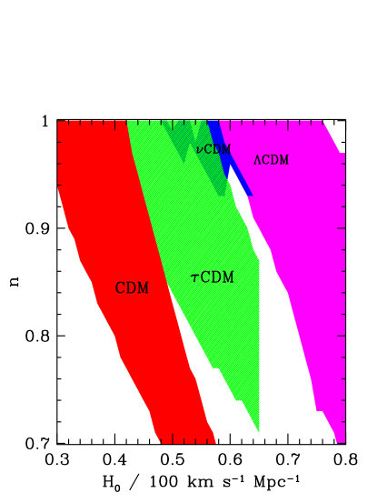
Figure 9: Acceptable values of the cosmological parameters $n$ and $h$ for CDM models with standard invisible-matter content (CDM), with 20% hot dark matter ($\nu$CDM), with additional relativistic particles (the energy equivalent of 12 massless neutrino species, denoted $\tau$CDM), and with a cosmological constant that accounts for 60% of the critical density ($\Lambda$CDM). A model is considered viable if it passes the three tests for any value of $\Omega_{B}h^{2}$ between $0.01$ and $0.02$ and any level of gravitational waves. The $\tau$CDM models have been truncated at a Hubble constant of $65\,{\rm km\,s^{-1}}\,{\rm Mpc}^{-1}$ because a larger value would result in a Universe that is younger than $10\,{\rm Gyr}$ (from Ref. [74]).

A host of other observations test CDM. Some are more controversial and/or open to interpretation. They tend to distinguish the cosmological-constant family of models from the other three families. This is because models with standard invisible matter, extra radiation, or a hot dark matter component are all matter dominated today and have the same kinematic properties – age for a given Hubble constant and distance to an object of given redshift. The introduction of a cosmological constant leads to an older Universe and greater distance to an object at fixed redshift.

Together, the Hubble constant and age of the Universe, have great leverage. Determinations of the Hubble constant based upon a variety of techniques (Type Ia and II supernovae, IR Tully-Fisher and fundamental-plane methods) have converged on a value between $60\,{\rm km\,s^{-1}}\,{\rm Mpc}^{-1}$ and $80\,{\rm km\,s^{-1}}\,{\rm Mpc}^{-1}$ [91]. This corresponds to an expansion age of less than $11\,{\rm Gyr}$ for a flat, matter-dominated model; for $\Lambda$CDM, the expansion age can be significantly higher, as large as $16\,{\rm Gyr}$ for $\Omega_{\Lambda}=0.6$ (see Fig. 7). On the other hand, the ages of the oldest globular clusters indicate that the Universe is between $13\,{\rm Gyr}$ and $17\,{\rm Gyr}$ old; further, these age determinations, together with the those for the oldest white dwarfs and the long-lived radioactive elements, provide an ironclad case for a Universe that is at least $10\,{\rm Gyr}$ old [92, 93, 94]. At face value, the age/Hubble constant combination favor $\Lambda$CDM. But again, I want to stress that, within the uncertainties in both the age and Hubble constant, all of the models are viable.

Clusters are large enough that the baryon fraction should reflect its “universal value,” $\Omega_{B}/\Omega_{M}=(0.007-0.024)h^{-2}/(1-\Omega_{\Lambda})$. Most of the (observed) baryons in clusters are in the hot, intracluster x-ray emitting gas. From x-ray measurements of the flux and temperature of the gas, baryon fractions in the range $(0.04-0.10)h^{-3/2}$ have been determined [95, 96, 97]; further, a recent detailed analysis and comparison to numerical models of clusters in CDM indicates an even smaller scatter, $(0.07\pm 0.007)h^{-3/2}$ [98]. From the cluster baryon fraction and $\Omega_{B}$, $\Omega_{M}$ can be inferred: $\Omega_{M}=(0.25\pm 0.15)h^{-1/2}$, which for the lowest Hubble constant consistent with current determinations ($h=0.6$) implies $\Omega_{M}=0.32\pm 0.2$. Unless one of the assumptions underlying this analysis is wrong, $\Lambda$CDM is strongly favored.

E. Turner emphasized the frequency of gravitational lensing of distant QSOs as an important cosmological test [99]. The underlying principle is simple: the comoving distance to fixed redshift depends upon the cosmology – it is largest for a cosmological constant, and in a matter-dominated Universe decreases with increasing $\Omega_{M}$ – and the probability of lensing increases with comoving distance (more lenses along the line of sight). For a flat Universe, Kochanek has obtained the upper limit $\Omega_{\Lambda}<0.65$ (95%), and for a matter-dominated Universe $0.25<\Omega_{M}<2$ (95%) [100]. Neither result is decisive.

$\Lambda$CDM is consistent with all the observations discussed here as well as others; see Fig. 10. For this reason, it is the strawman CDM model [101]. The parameters for this best fit model are: $\Omega_{\Lambda}\sim 0.5-0.65$ and $h\sim 0.6-0.7$. One should keep in mind that the introduction of a cosmological constant is a big step, one which twice before proved to be a misstep, and raises a fundamental question – the origin of the implied vacuum energy, about $10^{-8}{\,\rm eV}^{4}$ [76].

$\Lambda$CDM’s hold on the title of best-fit CDM model is by no means unshakeable: should the Hubble constant turn out to be less than $60\,{\rm km\,s^{-1}}\,{\rm Mpc}^{-1}$ and should a flaw be found in the cluster-baryon-fraction argument, the other models become very viable and are theoretically more attractive. Bartlett et al have pointed out that if the Hubble constant is around $30\,{\rm km\,s^{-1}}\,{\rm Mpc}^{-1}$, then CDM with $n\approx 1$ is consistent with all the measurements discussed above [102]. Lineweaver et al have analyzed the existing CBR anisotropy data and conclude that it favors a Hubble constant of around this value [103]. The rub is squaring this “determination” of $H_{0}$ with the multitude of other determinations that indicate a value almost twice as large. Appealing to a difference between the local value of the expansion rate and the global value is of little help – in the context of CDM, the difference, which arises due to cosmic and sampling variance, is expected to be only 10% or so [104].

Figure 10: Summary of constraints projected onto the $H_{0}$ – $\Omega_{M}$ plane: (CBF) comes from combining the BBN limit to the baryon density with x-ray observations of clusters; (PS) arises from the power spectrum; (AGE) is based on age determinations of the Universe; ($H_{0}$) indicates the range currently favored for the Hubble constant. The constraint $\Omega_{\Lambda}<0.66$ has been implicitly taken into account since the $\Omega_{\Lambda}$ axis extends only to 0.7. The darkest region indicates the parameters allowed by all constraints.

In finishing this status report I would like to emphasize three things. First, inflation is currently consistent with all the observational data, which is no mean feat. Second, cold dark matter is consistent with a large body of high-quality cosmological data, ranging from measurements of CBR anisotropy to our growing understanding of the evolution of galaxies and clusters of galaxies. This too is no mean feat; at the moment, the only other potentially viable paradigm for structure formation is topological defects + nonbaryonic dark matter. These models, when COBE normalized, appear to be in great jeopardy as they predict very little power on small scales (high bias). Finally, the quantity of high-quality data that bear on inflation and cold dark matter is growing rapidly, leading me to believe that inflation/cold dark matter will be decisively tested soon.

10 The Future: Precision Testing and More

Inflation is a bold attempt to build upon the success of the standard cosmology and extend our understanding of the Universe to times as early as $10^{-32}\,{\rm sec}$ after the bang. Its three robust predictions – flat Universe, nearly scale-invariant spectrum of density perturbations, and nearly scale-invariant spectrum of gravitationally waves – are the keys to its testing. In addition, much can be learned about the specific, underlying model of inflation if other measurements are made (e.g., the small anticipated deviation from scale invariance and the level of gravitational waves).

Cold dark matter, which is an important means of testing inflation, is a ten-parameter theory, $h$, $\Omega_{B}h^{2}$, $S$, $n$, $dn/d\ln k$, $T/S$, $n_{T}$, $\Omega_{\nu}$, $g_{*}$, and $\Omega_{\Lambda}$. While this is a daunting number of parameters, especially for a cosmological theory, there is good reason to believe that within ten years the data will overdetermine these parameters. Crucial to achieving this goal are the high-precision, high-resolution measurements of CBR anisotropy that will be made over the next decade by earth-based, balloon-borne and satellite-borne instruments (see Fig. 11). As a reminder of the power of high-quality data, the standard model of particle physics has nineteen parameters; precision measurements at Fermilab, SLAC, CERN and other accelerator laboratories, as well as nonaccelerator experiments, have both sharply tested the theory as well as accurately determining the parameters.

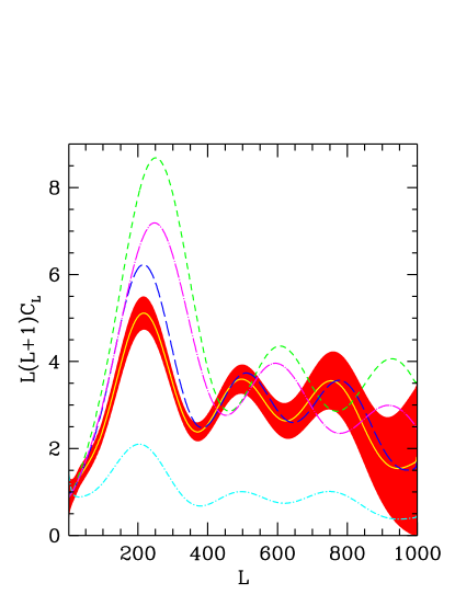
Figure 11: Predicted angular power spectra of CBR anisotropy for several viable CDM models and the anticipated uncertainty (per multipole) from a CBR satellite experiment similar to MAP. From top to bottom the CDM models are: CDM with $h=0.35$, $\tau$CDM with the energy equivalent of 12 massless neutrino species, $\Lambda$CDM with $h=0.65$ and $\Omega_{\Lambda}=0.6$, $\nu$CDM with $\Omega_{\nu}=0.2$, and CDM with $n=0.7$ (unspecified parameters have their standard CDM values) (from Ref. [74]).

Within five years we should be well on our way to precisely testing inflation and cold dark matter. In the next few years ground-based and balloon-borne anisotropy experiments (e.g., VSA, VCA, Boomerang, TOPHAT, QMAX, and others) should be able to determine the approximate position of the Doppler peak and thereby $\Omega_{0}$ to an accuracy of around 10%. Because flatness is a fundamental prediction of inflation, perhaps the most fundamental, this is a landmark test. On the same timescale, the Supernova Cosmology Project and the High-Redshift Supernova Team will use the SNeIa magnitude – redshift diagram to determine the deceleration of the Universe. While the Doppler peak determines $\Omega_{M}+\Omega_{\Lambda}$, the SNeIa measurement determines an almost orthogonal quantity, $\Omega_{M}-\Omega_{\Lambda}$; together, they can determine $\Omega_{M}$ and $\Omega_{\Lambda}$.

In the same time frame measurements of the Hubble constant will play an important role. Since the Universe is at least $10\,{\rm Gyr}$ old, a definitive determination that the Hubble constant is $65\,{\rm km\,s^{-1}}\,{\rm Mpc}^{-1}$ or greater would rule out all models but $\Lambda$CDM; on the other hand, a determination that the Hubble constant is below $55\,{\rm km\,s^{-1}}\,{\rm Mpc}^{-1}$ would undermine much of the motivation for $\Lambda$CDM. The Hubble Space Telescope calibration of secondary distance indicators such as SNeIa with Cepheids in nearby galaxies and the maturation of physics-based methods such as gravitational time delay and Zel’dovich – Sunyaev are helping to pin down $H_{0}$ more accurately [105].

There are other important tests that will be made on a longer time scale. The level of inhomogeneity in the Universe today is determined mainly from redshift surveys, the largest of which contains of order $30,000$ galaxies. Two larger surveys are underway. The Sloan Digital Sky Survey will cover 25% of the sky and obtain positions for two hundred million galaxies and redshifts for a million galaxies [106]. The Anglo – Australian Two-degree Field is targeting hundreds of two-degree patches on the sky and will obtain 250,000 redshifts [107]. These two projects will determine the power spectrum much more precisely and on scales large enough ($500h^{-1}\,{\rm Mpc}$) to connect with measurements from CBR anisotropy on angular scales of up to five degrees, allowing bias to be probed.

The most fundamental element of cold dark matter – the existence of the CDM particles – will be tested over the next decade. Experiments with sufficient sensitivity to detect the CDM particles that hold our own galaxy together if they are in the form of axions of mass $10^{-6}{\,\rm eV}-10^{-4}{\,\rm eV}$ [81] or neutralinos of mass tens of GeV [82] are now underway. Evidence for the existence of the neutralino could also come from particle accelerators searching for other supersymmetric particles [108]. In addition, a variety of experiments sensitive to neutrino masses are operating or are planned: accelerator-based neutrino oscillation experiments at Fermilab, CERN, and Los Alamos; solar-neutrino detectors in Japan, Canada, Germany, Russia and Italy; and experiments at $e^{+}e^{-}$ colliders (LEP at CERN and CESR at Cornell) to the study the tau neutrino.

The most telling test of inflation and cold dark matter will come with the two new space missions that have recently been approved – MAP to be launched in 2000 by NASA and Planck to launched by ESA in 2005. Each will map CBR anisotropy over the entire sky with more than thirty times the angular resolution of COBE (resolution of $0.2^{\circ}$ for MAP and $0.1^{\circ}$ for Planck). MAP should determine the angular power spectrum out to multipole number 1000, and Planck out to multipole number 2000, each to a precision close to that dictated by sampling variance alone. Theoretical studies [109] indicate that the results of Planck should be able to determine $n$ to a precision of less than one percent, $\Omega_{\Lambda}$ to a few percent, $\Omega_{0}$ to less than one percent, $\Omega_{\nu}$ to enough precision to test $\nu$CDM [110], the baryon density to less than ten percent, and even the Hubble constant to one percent.

Inflation and cold dark matter are a bold attempt to extend our knowledge of the Universe to within $10^{-32}\,{\rm sec}$ of the bang. The number of observations that are testing the cold dark matter theory is growing fast, and prospects for not only testing the theory, but also discriminating among the different CDM models and models of inflation are excellent. If cold dark matter is shown to be correct, an important aspect of the standard cosmology – the origin and evolution of structure – will have been resolved and a window to the early moments of the Universe and physics at very high energies will have been opened.

While the window has not been opened yet, I would like to end with one example of what one could hope to learn. As discussed earlier, $S$, $n-1$, $T/S$ and $n_{T}$ are related to the inflationary potential and its first two derivatives. If one can measure the power-law index of the scalar perturbations and the amplitudes of the scalar and tensor perturbations, one can recover the value of the potential and its first two derivatives around the point on the potential where inflation took place [62]:

$$V_{*} = 1.65T\,{m_{\rm Pl}}^{4},$$ (20)

$$V_{*}^{\prime} = \pm\sqrt{{8\pi\over 7}\,{T\over S}}\,V_{*}/{m_{\rm Pl}},$$ (21)

$$V_{*}^{\prime\prime} = 4\pi\left[(n-1)+{3\over 7}{T\over S}\right]\,V_{*}/{m_{\rm Pl}}^{2},$$ (22)

where the sign of $V^{\prime}$ is indeterminate (under $\phi\leftrightarrow-\phi$ the sign changes). If the tensor spectral index can also be measured the relation, $T/S=-7n_{T}$, can be used to test the consistency of inflation. Reconstruction of the inflationary scalar potential would shed light both on inflation as well as physics at energies of the order of $10^{14}\,{\rm GeV}$.

Acknowledgments.

Much of the material in these lectures derives from collaborative work with Scott Dodelson, Evalyn Gates, Lloyd Knox, Andrew Liddle, and Martin White. I thank my collaborators for teaching me so much. This work was supported by the DoE (at Chicago and Fermilab) and by the NASA (at Fermilab by grant NAG 5-2788).

References

- [1] See e.g., P.J.E. Peebles, Physical Cosmology (Princeton University Press, Princeton, 1993).
- [2] A.H. Guth, Phys. Rev. D 23, 347 (1981).
- [3] A. H. Guth and S.-Y. Pi, Phys. Rev. Lett. 49, 1110 (1982); S. W. Hawking, Phys. Lett. B 115, 295 (1982); A. A. Starobinskii, ibid 117, 175 (1982); J. M. Bardeen, P. J. Steinhardt, and M. S. Turner, Phys. Rev. D 28, 697 (1983).
- [4] M.S. Turner and L.M. Widrow, Phys. Rev. Lett. 57, 2237 (1986); L. Jensen and J. Stein-Schabes, Phys. Rev. D 35, 1146 (1987); A.A. Starobinskii, JETP Lett. 37, 66 (1983).
- [5] See e.g., A.D. Linde, Inflation and Quantum Cosmology (Academic Press, San Diego, CA, 1990); or A. Vilenkin, Phys. Rev. D 52, 3365 (1995).
- [6] R. Penrose, in General Relativity: An Einstein Centenary Survey, edited by S.W. Hawking and W. Israel (Cambridge University Press, Cambridge), p. 581.
- [7] Y. Hu, M.S. Turner, and E.J. Weinberg, Phys. Rev. D 49, 3830 (1994); A.R. Liddle, ibid 51, 5347 (1995).
- [8] See e.g., E.W. Kolb and M.S. Turner, The Early Universe (Addison-Wesley, Redwood City, 1990), Ch. 8.
- [9] A.D. Linde, Phys. Lett. B 129, 177 (1983).
- [10] Q. Shafi and A. Vilenkin, Phys. Rev. Lett. 52, 691 (1984); S.-Y. Pi, ibid 52, 1725 (1984).
- [11] R. Holman, P. Ramond, and G.G. Ross, Phys. Lett. B 137, 343 (1984).
- [12] K. Olive, Phys. Repts. 190, 309 (1990).
- [13] H. Murayama et al., Phys. Rev. D(RC) 50, R2356 (1994).
- [14] M. Cvetic, T. Hubsch, J. Pati, and H. Stremnitzer, Phys. Rev. D 40, 1311 (1990).
- [15] E.J. Copeland et al., Phys. Rev. D 49, 6410 (1994).
- [16] See e.g., M. Gasperini and G. Veneziano, Phys. Rev. D 50, 2519 (1994); R. Brustein and G. Veneziano, Phys. Lett. B 329, 429 (1994); T. Banks et al., Phys. Rev. D 52, 3548 (1995).
- [17] K. Freese, J.A. Frieman, and A. Olinto, Phys. Rev. Lett. 65, 3233 (1990); L. Randall, M. Soljacic, and A. Guth, Nucl. Phys. B 472, 377 (1996).
- [18] L. Knox and M.S. Turner, Phys. Rev. Lett. 70, 371 (1993).
- [19] J. Silk and M.S. Turner, Phys. Rev. D 35, 419 (1986); L.A. Kofman, A.D. Linde, and J. Einsato, Nature 326, 48 (1987).
- [20] D. La and P.J. Steinhardt, Phys. Rev. Lett. 62, 376 (1991).
- [21] E.W. Kolb, Physica Scripta T36, 199 (1991).
- [22] A. Albrecht et al, Phys. Rev. Lett. 48, 1437 (1982); L. Abbott and M. Wise, Phys. Lett. B 117, 29 (1992); A.D. Linde and A.D. Dolgov, ibid 116, 329 (1982).
- [23] See e.g., L. Kofman et al., Phys. Rev. Lett. 73, 3195 (1994); 76, 1011 (1996); E.W. Kolb et al., ibid 77, 4290 (1996); S. Khebnikov and I. Tkachev, ibid 77, 219 (1996); D. Boyanovsky et al, hep-ph/9701304.
- [24] V.A. Rubakov, M. Sazhin, and A. Veryaskin, Phys. Lett. B 115, 189 (1982); R. Fabbri and M. Pollock, ibid 125, 445 (1983); A.A. Starobinskii Sov. Astron. Lett. 9, 302 (1983); L. Abbott and M. Wise, Nucl. Phys. B 244, 541 (1984).
- [25] M.S. Turner and F. Wilczek, Phys. Rev. Lett. 65, 3080 (1990); A. Kosowsky, M.S. Turner, and R. Watkins, ibid 69, 2026 (1992).
- [26] M.S. Turner and L.M. Widrow, Phys. Rev. D 37, 2743 (1988); B. Ratra, Astrophys. J. 391, L1 (1992).
- [27] See e.g., A. Vilenkin, astro-ph/9610125.
- [28] See e.g., A.D. Linde, Phys. Lett. B 158, 375 (1985); D. Seckel and M.S. Turner, Phys. Rev. D 32, 3178 (1985).
- [29] M.S. Turner, A. Cohen, and D. Kaplan, Phys. Lett. B 216, 20 (1989).
- [30] P.J.E. Peebles, astro-ph/9704xxx (Astrophys. J., in press).
- [31] M.S. Turner, Phys. Rev. D 44, 3737 (1991).
- [32] M. Bucher A.S. Goldhaber, and N. Turok, Phys. Rev. D 52, 3314 (1995); A.D. Linde and A. Mezhlumian, ibid 52, 6789 (1995); J.R. Gott, Nature 295, 304 (1992); A. Green and A. Liddle, Phys. Rev. D 55, 609 (1997)
- [33] J.R. Gott, Nature 295, 304 (1992); A.H. Guth and E.J. Weinberg, Nucl. Phys. B 212, 321 (1983).
- [34] A. Vilenkin and S. Winitzki, Phys. Rev. D 55, 548 (1997).
- [35] C. Copi, D.N. Schramm, and M.S. Turner, Science 267, 192 (1995).
- [36] D. Tytler, X.-M. Fan and S. Burles, Nature 381, 207 (1996); D. Tytler, S. Burles and D. Kirkman, astro-ph/9612121.
- [37] Y. Sigad et al, in preparation (1997); J. Willick et al, astro-ph/96 A. Dekel, D. Burstein, and S. White, astro-ph/9611108. M. Strauss and J. Willick, Phys. Repts. 261, 271 (1995); A. Dekel, Ann. Rev. Astron. Astrophys. 32, 319 (1994); N. Bahcall, L.M. Lubin and V. Dorman, Astrophys. J. 447, L81 (1995); A. Dekel and M.J. Rees, Astrophys. J. 422, L1 (1994); R.G. Carlberg, H.K.C. Yee, and E. Ellingson, astro-ph/9512087.
- [38] See e.g., M.S. Turner, Phys. Rept. 197, 67 (1990); G.G. Raffelt, ibid 198, 1 (1990).
- [39] See e.g., G. Jungman, M. Kamionkowski, and K. Griest, Phys. Rept. 267, 195 (1996).
- [40] See e.g., G.G. Ross, Grand Unified Theories (Addison-Wesley, Redwood City, 1985), or B. Kayser, F. Gibrat-Debu, and F. Perrier, The Physics of Massive Neutrinos (World Scientific, Singapore, 1989).
- [41] A. Vilenkin, Phys. Rev. Lett. 53, 1016 (1984); M.S. Turner, G. Steigman, and L. Krauss, Phys. Rev. Lett. 52, 2090 (1984); R.L. Davis, Phys. Rev. D 35, 3705 (1987); M. Kamionkowski and N. Toumbas, Phys. Rev. Lett. 77, 587 (1996); M. Ozer and M.O. Taha, Nucl. Phys. B287 776 (1987); K. Freese et al., Nucl. Phys. B287 797 (1987); B. Ratra and P.J.E. Peebles, Phys. Rev. D 37, 3406 (1988); L.F. Bloomfield-Torres and I. Waga, astro-ph/9504101; K. Coble, S. Dodelson, and J. Frieman, Phys. Rev. D 55, 1851 (1996).
- [42] G.F. Smoot et al., Astrophys. J. 396, L1 (1992).
- [43] J.M. Bardeen, J.R. Bond, N. Kaiser, and A.S. Szalay, Astrophys. J., 304, 15 (1986).
- [44] A.R. Liddle and M.S. Turner, Phys. Rev. D 54, 2980 (1996).
- [45] M.S. Turner and M. White, Phys. Rev. D 53, 6822 (1996).
- [46] P.J. Steinhardt and M.S. Turner, Phys. Rev. D 29, 2162 (1984).
- [47] M.S. Turner, Phys. Rev. D 48, 3502 (1993).
- [48] D.H. Lyth and A.R. Liddle, Phys. Lett. B 291, 391 (1992).
- [49] A.D. Linde, Phys. Lett. B 108, 389 (1982); A. Albrecht and P.J. Steinhardt, Phys. Rev. Lett. 48, 1220 (1982).
- [50] D.H. Lyth and E. Stewart, Phys. Rev. D 54, 7186 (1996); A. Linde, ibid 49, 748 (1994).
- [51] A. Kosowsky and M.S. Turner, Phys. Rev. D 52, R1739 (1995).
- [52] J. Bartlett et al., Science 267, 980 (1995); P.T.P. Viana et al., Mon. Not. R. astron. Soc. 283, 107 (1996).
- [53] See e.g., W. Hu and N. Sugiyama, Phys. Rev. D 51, 2599 (1991). For a very fast and accurate numerical routine, see U. Seljak and M. Zaldarriaga, astro-ph/9603033.
- [54] R.K. Sachs and A.M. Wolfe, Astrophys. J. 147, 73 (1967).
- [55] C.L. Bennett et al, Astrophys. J. 464, L1 (1996).
- [56] E.F. Bunn et al., Phys. Rev. D 54, 5917 (1997); also see e.g., K. Gorski et al, astro-ph/9608054.
- [57] R.H. Dicke and P.J.E. Peebles, in General Relativity: An Einstein Centenary Survey, edited by S.W. Hawking and W. Israel (Cambridge University Press, Cambridge), p. 504.
- [58] E.R. Harrison, Phys. Rev. D 1, 2726 (1970); Ya.B. Zel’dovich, Mon. Not. R. astr. Soc. 160, 1p (1972).
- [59] See e.g., M.S. Turner, J.E. Lidsey and M. White, Phys. Rev. D 48, 4613 (1993).
- [60] M.S. Turner and Y. Wang, Phys. Rev. D 53, 5727 (1996); B. Allen and S. Koranda, ibid 52, 1902 (1995); S. Dodelson et al, Phys. Rev. Lett. 72, 3444 (1994); R. Crittenden et al, ibid 71, 324 (1993).
- [61] R. Davis et al., Phys. Rev. Lett. 69, 1856 (1992); F. Lucchin, S. Mattarese, and S. Mollerach, Astrophys. J. 401, L49 (1992); D. Salopek, Phys. Rev. Lett. 69, 3602 (1992); A. Liddle and D. Lyth, Phys. Lett. B 291, 391 (1992); J.E. Lidsey and P. Coles, Mon. Not. R. astron. Soc. 258, 57p (1992); T. Souradeep and V. Sahni, Mod. Phys. Lett. A 7, 3541 (1992).
- [62] See e.g., E.J. Copeland, E.W. Kolb, A.R. Liddle, and J.E. Lidsey, Phys. Rev. Lett. 71, 219 (1993); Phys. Rev. D 48, 2529 (1993); M.S. Turner, ibid, 3502 (1993); ibid 48, 5539 (1993); S. Dodelson, W.H. Kinney and E.W. Kolb, astro-ph/9702166.
- [63] L. Knox and M.S. Turner, Phys. Rev. Lett. 73, 3347 (1994).
- [64] U. Seljak, astro-ph/9608131; M. Kamionkowski, A. Kosowsky, and A. Stebbins, astro-ph/9609132.
- [65] M.S. Turner, Phys. Rev. D 55, R435 (1997).
- [66] See e.g., A. Abramovici et al., Science 256, 325 (1992) and in Particle and Nuclear Astrophysics and Cosmology in the Next Millennium, eds. E.W. Kolb and R.D. Peccei (World Scientific, Singapore, 1995), p. 398; N. Christensen, Phys. Rev. D 46, 5250 (1992); E. Flanagan, ibid 48, 2389 (1993).
- [67] B. Allen, qr-gc/9604033.
- [68] Pre-phase A Design Study for LISA.
- [69] K.S. Thorne, in 300 Years of Gravitation, eds. S.W. Hawking and W. Israel (Cambridge Univ. Press, Cambridge, 1987), p.330.
- [70] S.D.M. White, C. Frenk and M. Davis, Astrophys. J. 274, L1 (1983).
- [71] S. Colombi, S. Dodelson and L. Widrow, Astrophys. J. 458, 1 (1996).
- [72] G. Blumenthal et al., Nature 311, 517 (1984).
- [73] See e.g., J.P. Ostriker and R. Cen, astro-ph/9601021; Y. Zhang et al, astro-ph/9711224; T. Abel et al, astro-ph/9608040;
- [74] S. Dodelson, E. Gates and M.S. Turner, Science 274, 69 (1996).
- [75] For example, S. Parke, Phys. Rev. Lett. 74, 839 (1995); C. Athanassopoulos et al, ibid 75, 2650 (1995); J.E. Hill, ibid, 2654 (1995); K.S. Hirata et al, Phys. Lett. B 280, 146 (1992); Y. Fukuda et al, ibid 335, 237 (1994); R. Becker-Szendy et al, Phys. Rev. D 46, 3720 (1992).
- [76] S. Weinberg, Rev. Mod. Phys. 61, 1 (1989).
- [77] K. Fisher et al., Mon. Not. R. astron. Soc. 266, 50 (1994).
- [78] S. Hancock and G. Rocha, astro-ph/9612016.
- [79] S.J. Perlmutter et al, astro-ph/9608192.
- [80] M.S. Turner and M. White, astro-ph/9701138.
- [81] C. Hagmann et al, Nucl. Phys. B (Proc. Suppl.) 51, 209 (1996).
- [82] T. Shutt et al, in Proceedings of the XVIIIth Texas Symposium on Relativistic Astrophysics (Chicago, IL, 1996), edited by A. Olinto (World Scientific, Singapore, 1997).
- [83] J. Peacock and S. Dodds, Mon. Not. Roy. astron. Soc. 267, 1020 (1994).
- [84] A.R. Liddle et al., Mon. Not. R. astron. Soc. 282, 281 (1996); ibid 281, 531 (1995); J.S. Bagla, T. Padmanabhan and J.V. Narlikar, astro-ph/9511102; S. Cole et al, astro-ph/9702082.
- [85] S.D.M. White, G. Efstathiou, and C.S. Frenk, Mon. Not. Roy. astron. Soc. 262, 1023 (1993).
- [86] R. Carlberg et al., J. R. Astron. Soc. Canada 88, 39 (1994); P.T.P. Viana and A. Liddle, Mon. Not. R. astron. Soc. 281, 323 (1996); J.R. Bond and S. Myers, Astrophys. J. Supp. 103, 63. (1996); V.R. Eke, S. Cole and C.S. Frenk, astro-ph/9601088; U.-L.Pen, astro-ph/9610147.
- [87] K. Lanzetta, A.M. Wolfe, and D.A. Turnshek, Astrophys. J. 440, 435 (1995); L.J. Storrie-Lombardi, R.G. McMahon, M.J. Irwin, and C. Hazard, astro-ph/9503089 (1996).
- [88] J.P. Ostriker, Ann. Rev. Astron. Astrophys. 31, 689 (1993).
- [89] A. Liddle and D. Lyth, Phys. Repts. 231, 1 (1993).
- [90] M. White and J. Silk, Phys. Rev. Lett. 77 4704 (1996).
- [91] See e.g., W. Freedman, astro-ph/9612024; A. Riess, R.P. Krishner, and W. Press, Astrophys. J. 438, L17 (1995); R. Giovanelli et al, astro-ph/9612072.
- [92] M. Bolte and C.J. Hogan, Nature 376, 399 (1995).
- [93] B. Chaboyer et al, Science 271, 957 (1996).
- [94] J. Cowan, F. Thieleman, and J. Truran, Ann. Rev. Astron. Astrophys. 29, 447 (1991).
- [95] S.D.M. White et al, Nature 366, 429 (1993).
- [96] U.G. Briel et al, Astron. Astrophys. 259, L31 (1992).
- [97] D.A. White and A.C. Fabian, Mon. Not. R. astron. Soc. 273, 72 (1995).
- [98] A. Evrard, astro-ph/9701148.
- [99] E. Turner, Astrophys. J. 365, L43 (1990).
- [100] C.S. Kochanek, Astrophys. J. 466, 638 (1996).
- [101] L. Krauss and M.S. Turner, Gen. Rel. Grav. 27, 1137 (1995); J.P. Ostriker and P.J. Steinhardt, Nature 377, 600 (1995); J.S. Bagla, T. Padmanabhan and J.V. Narlikar, astro-ph/9511102; A.R. Liddle et al., Mon. Not. R. astron. Soc. 282, 281 (1996).
- [102] J. Bartlett et al., Science 267, 980 (1995);
- [103] C.H. Lineweaver, D. Barbosa, A. Blanchard, and J. Bartlett, astro-ph/9612146.
- [104] See e.g., E.L. Turner, R. Cen, and J.P. Ostriker, Astron. J. 103, 1427 (1992); X. Shi, L.M. Widrow, and L.J. Dursi, Mon. Not. R. astron. Soc. 281, 565 (1996); X. Shi and M.S. Turner, astro-ph/9705xxx.
- [105] T. Kundic et al, astro-ph/9610162; P.L. Schechter et al, astro-ph/9611051; W.L. Holzapfel et al, astro-ph/9702224; S.T. Meyers et al, astro-ph/9703123.
- [106] See http://www-sdss.fnal.gov:8000/.
- [107] See http://www.ast.cam.ac.uk/AAO/2df.
- [108] See e.g., J.E. Ellis, Physics World, July 1994, p. 31.
- [109] See e.g., L. Knox, Phys. Rev. D 52, 4307 (1995); G. Jungman, M. Kamionkowski, A. Kosowsky, and D. Spergel, Phys. Rev. D 54, 1332 (1996); J.R. Bond, G. Efstathiou, and M. Tegmark, astro-ph/0702100; M. Zaldarriaga, D.Spergel and U. Seljak, astro-ph/9702157.
- [110] S. Dodelson, E. Gates, and A.S. Stebbins, Astrophys. J. 467, 10 (1996).