Fluctuations in the IRAS 1.2 Jy Catalogue

Abstract

An analysis of the IRAS 1.2 Jy redshift catalogue with emphasis on the separate examination of northern and southern parts (in galactic coordinates) is performed using a complete set of morphological descriptors (Minkowski functionals), nearest neighbour distributions and the variance of the galaxy counts. We find large fluctuations in the clustering properties as seen in a large difference between the northern and southern parts of the catalogue on scales of 100$h^{-1}$Mpc. These fluctuations remain discernible even on the scale of 200$h^{-1}$Mpc. We also identify sparse sampling as a major source of “apparent homogenization”. Tests on observational selection effects concerning luminosity, colour and redshift–space distortion support the significance of these large–scale fluctuations.

1 Introduction

The spatial distribution of luminous matter seen in the available galaxy redshift catalogues conveys a complex picture of voids, isolated galaxies, clusters and superclusters, with the largest filamentary features extending on scales comparable with the size of the surveys. Since these findings are expected to provide important constraints for theoretical models of structure evolution, a prime task is to extract the morphological characteristics of the observed patterns by appropriate quantitative measures.

In the present paper we consider the IRAS 1.2 Jy catalogue Fisher et al. (1995). This infrared–selected survey consists of two data sets for the northern and southern caps (in galactic coordinates) separated by a 10 degree wide zone of avoidance and is therefore nearly all–sky. We analyze the two subsamples individually with Minkowski functionals Mecke et al. (1994) in order to quantify the global geometrical and topological features of spatial patterns. In addition, we apply a novel method of cluster diagnostics van Lieshout and Baddeley (1996) combining local and global statistical descriptors, and the more conventional count–in–cell method.

Practically, when analyzing galaxy surveys one has to deal with various technical problems. As a rule, three–dimensional galaxy catalogues are constructed from redshift surveys which suffer from distortions due to peculiar motions. To date, there is no way of tackling this problem without making strong assumptions (e.g. linearized equations of motion), and therefore we conduct our analysis in redshift space and investigate the differences to real space by comparing with results of $N$–body simulations. Furthermore, surveys are usually flux limited. Therefore, the observed number density of the galaxies decreases with distance. For samples with inhomogeneous mean number density the methods employing morphological estimators are usually dominated by thinning at the fringes. One remedy is to focus on volume limited subsamples, at the cost of losing a substantial fraction of galaxies. Nevertheless, we show that Minkowski functionals provide significant results even for a small number of galaxies. Finally, all surveys are spatially limited both in directions as well as in depth, where volume limitation leads to a well–defined spherical boundary. Hence, we have to take care of boundary constraints. In Appendix A we discuss these finite size effects on the estimators for the Minkowski functionals, for the nearest–neighbour distribution, and for the fluctuations of the galaxy counts.

As a result we detect a significant morphological segregation between the northern and the southern part of the IRAS catalogue. These findings are also supported by our further results on the variances of counts in cells, done separately for the north and the south.

2 Methods of morphological analysis

We consider a set $X=\{{\mathbf{x}}_{i}\}_{i=1}^{N}$ of $N$ points ${\mathbf{x}}_{i}\in{\mathbb{R}}^{3}$ given by the redshift–space coordinates of the galaxies in the IRAS 1.2 Jy catalogue Fisher et al. (1995).

2.1 Minkowski functionals

A computationally convenient and robust method for quantifying the morphology of spatial patterns is offered by Minkowski functionals as they were introduced into cosmology by ?. For this purpose we decorate each point ${\mathbf{x}}_{i}$ with a ball ${\mathcal{B}}_{r}({\mathbf{x}}_{i})$ of radius $r$ and then consider the union set ${\mathcal{A}}_{N}(r)=\bigcup_{i=0}^{N}{\mathcal{B}}_{r}({\mathbf{x}}_{i})$. ? proved that in three dimensions the four Minkowski functionals $M_{\mu=0,1,2,3}({\mathcal{A}}_{N}(r))$ give a complete morphological characterization of a body ${\mathcal{A}}_{N}(r)$. The interpretation of these functionals in terms of geometrical and topological quantities is given in Table (1).

Table 1: Minkowski functionals in three–dimensional space expressed in terms of more familiar geometric quantities.

	geometric quantity	$\mu$	$M_{\mu}$	$\Phi_{\mu}$
$V$	volume	0	$V$	$V/(\tfrac{4\pi}{3}r^{3}N)$
$A$	surface	1	$A/8$	$A/(4\pi r^{2}N)$
$H$	integral mean curvature	2	$H/(2\pi^{2})$	$H/(4\pi rN)$
$\chi$	Euler characteristic	3	$3\chi/(4\pi)$	$\chi/N$

By normalizing with the functional $M_{\mu}({\mathcal{B}}_{r})$ of a single ball we can introduce normalized, dimensionless Minkowski functionals $\Phi_{\mu}({\mathcal{A}}_{N}(r))$,

$$\Phi_{\mu}({\mathcal{A}}_{N}(r)):=\frac{M_{\mu}({\mathcal{A}}_{N}(r))}{NM_{\mu}({\mathcal{B}}_{r})}.$$ (1)

In the case of a Poisson process the exact mean values of the functionals can be calculated analytically Mecke and Wagner (1991). For decorating spheres with radius $r$ one obtains:

$$\begin{split}\Phi_{0}^{\rm P}&=\left(1-{\rm e}^{-\eta}\right)\leavevmode\nobreak\ \eta^{-1},\\ \Phi_{1}^{\rm P}&={\rm e}^{-\eta},\\ \Phi_{2}^{\rm P}&={\rm e}^{-\eta}\leavevmode\nobreak\ (1-\tfrac{3\pi^{2}}{32}\eta),\\ \Phi_{3}^{\rm P}&={\rm e}^{-\eta}\leavevmode\nobreak\ (1-3\eta+\tfrac{3\pi^{2}}{32}\eta^{2}),\end{split}$$ (2)

with the dimensionless parameter $\eta=\overline{n}M_{0}({\mathcal{B}}_{r})=\overline{n}\ 4\pi r^{3}/3$, where $\overline{n}$ denotes the mean number density.

For $\mu\geq 1$ the measures $\Phi_{\mu}({\mathcal{A}}_{N}(r))$ contain the exponentially decreasing factor ${\rm e}^{-\eta(r)}$. It can be shown that this exponential decrease with increasing (diagnostic) radius $r$ also arises for more general cluster processes. Therefore we employ the reduction

$$\phi_{\mu}({\mathcal{A}}_{N}(r))=\frac{\Phi_{\mu}({\mathcal{A}}_{N}(r))}{\Phi_{1}^{\rm P}({\mathcal{A}}_{N}(r))},\quad\mu\geq 1,$$ (3)

and thereby remove the exponential decay and enhance the visibility of differences in the displays shown below.

2.2 Nearest neighbour statistics

The nearest neighbour distribution $G(r)$ is a standard tool in the analysis of point processes Ripley (1988) and is defined as the distribution of distances $r$ of a point of the process to the nearest other point of the process. The function $G(r)$ is related to conditional correlation functions White (1979). Another common statistical descriptor is the empty space function $F(r)$, the distribution of the distances $r$ of an arbitrary point to the nearest point of the process, and is equal to the expected fraction of volume occupied by points which are less distant than $r$ from the next point of the process. Therefore, $F(r)$ is equal to the volume density of $M_{0}({\mathcal{A}}_{N}(r))$; hence $1-F(r)$ coincides with the void probability function $P_{0}(r)$ White (1979). Alternatively, one may interpret $F(r)$ as the unconditional and $G(r)$ as the conditional distribution of the nearest neighbour distance. Recently, ? advocated to use the ratio

$$J(r):=\frac{1-G(r)}{1-F(r)}$$ (4)

as a probe for clustering of a point process. In the case of a Poisson process,

$$G^{\rm P}(r)=1-\exp(-\eta)=F^{\rm P}(r),$$ (5)

and thus $J^{\rm P}(r)=1$. For a process with enhanced clumping, we have $J(r)<1$, whereas regular structures are indicated by $J(r)>1$.

2.3 Fluctuations of the galaxy counts

Another frequently used method for exploring galaxy catalogues is to consider the fluctuations of galaxy counts, in particular, the variance of counts in cells in excess of Poisson,

$$\left\langle(N_{i}-\overline{n}V)^{2}\right\rangle=\overline{n}V+\overline{n}^{2}V^{2}\sigma^{2},$$ (6)

where $N_{i}$ is the number of galaxies in a volume V, in our case a ball ${\mathcal{B}}_{r}$ with radius $r$; the averaging is performed over random positions of the balls. For a Poisson process, $\sigma^{2}=0$ by definition. For stationary point processes the variance $\sigma^{2}$ is related to the two–point correlation function $\xi(r)$,

$$\sigma^{2}=\frac{1}{V^{2}}\int_{V}\int_{V}{\rm d}^{3}x{\rm d}^{3}y\,\xi(|x-y|).$$ (7)

After averaging a power–law correlation function $\xi(r)=(r_{0}/r)^{\gamma}$ over balls ${\mathcal{B}}_{r}$ one obtains Peebles (1993):

$$\sigma^{2}(r)=\Big{(}\frac{r_{0}}{2r}\Big{)}^{\gamma}\frac{1}{(1-\gamma/3)(1-\gamma/4)(1-\gamma/6)}.$$ (8)

In Appendix B we discuss the dependence of the variance $\sigma^{2}$ on the mean number density and we point out how this has to be modified for fractal sets.

3 Results

We now apply the methods introduced above to explore a redshift catalogue of 5313 IRAS selected galaxies with limiting flux of 1.2 Jy Fisher et al. (1995).

3.1 Volume limited samples with 100$h^{-1}$Mpc depth

A volume limited sample of 100$h^{-1}$Mpc  depth (with $h$ defined by $H_{0}=100h\ {\rm km}\ {\rm s}^{-1}\ {\rm Mpc}^{-1}$) contains 352 galaxies in the northern part, and 358 galaxies in the southern part. In Fig. 1 we see that the redshift and flux distributions of the galaxies do not indicate any peculiarity or problem with the sample. As far as the number density, i.e. the first moment of the galaxy distribution is concerned, the sample does not reveal differences between north and south. However, we want to assess the clustering properties of the data and, above all, tackle the question whether the southern and northern parts differ or not. More refined measurement of the galaxy distribution need to incorporate at least the second moment (see Sect. 3.1.5, 3.2.2). A complete characterization of morphology, depending on all moments of the distribution, is even more desirable. It is provided by the Minkowski functionals.

Figure 1: In the top panel we show the histograms of the redshift distribution of the galaxies for the volume limited sample with 100$h^{-1}$Mpc  depth. In the bottom panel we show the histograms for the flux distribution. The northern part is shown as a solid line, and the southern part as a dashed line.

3.1.1 Minkowski functionals

Figure 2: Minkowski functionals $\phi_{\mu}$ of a volume limited sample with 100$h^{-1}$Mpc  depth; the dark shaded areas represent the southern part, the medium shaded the northern part, and the dotted a Poisson process with the same number density. The shaded areas are the $1\sigma$ errors as explained in the text.

In Fig. 2 we show the values of the Minkowski functionals of the southern and northern parts, together with the values from a Poisson process with the same number density (the volume density is shown in Fig. 6). The errors for the Poisson process were calculated using twenty different realizations. This already gives a stable estimate of the ensemble variance. To estimate the error for the catalogue data we calculated the Minkowski functionals of twenty subsamples containing 90% of the galaxies, randomly chosen from the volume limited subsample.

In both parts of the 1.2 Jy catalogue the clustering of galaxies on scales up to 10$h^{-1}$Mpc  is clearly stronger than in the case of a Poisson process, as inferred from the lower values of the functionals for the surface area, $\phi_{1}$, the integral mean curvature, $\phi_{2}$, and the Euler characteristic, $\phi_{3}$. Moreover, the northern and southern parts differ significantly, with the northern part being less clumpy. The most conspicuous features are the enhanced surface area $\phi_{1}$ in the southern part on scales from 12 to 20$h^{-1}$Mpc and the kink in the integral mean curvature $\phi_{2}$ at 14$h^{-1}$Mpc. This behavior indicates that dense substructures in the southern part are filled up at this scale (i.e. the balls in these substructures overlap without leaving holes), and is presumably the signature of the Perseus–Pisces supercluster (for a more detailed analysis see ?). On scales from 15 to 20$h^{-1}$Mpc, $\phi_{2}$, the value of the integral mean curvature is negative, indicating concave structures. In the southern part the Euler characteristic is still negative in this range; therefore, the structure is dominated by interconnected tunnels (giving rise to negative contributions to the Euler characteristic) rather than by completely enclosed voids (these would result in positive contributions to the Euler characteristic). A similar feature is seen in the Minkowski functionals of Abell/ACO clusters Kerscher et al. (1997).

3.1.2 Error estimates

To get an impression how the error from subsampling is related to the intrinsic variance of an ensemble we looked at fixed realizations of a Poisson process within the sample geometry and calculated the error via subsampling using again 90% of the points. This error turns out to be two times smaller than the ensemble error calculated over different realizations of a Poisson process.

As for a further error estimate we randomize the redshifts using the quoted redshift errors as the standard deviation (and using the mean redshift error, if none is quoted). These errors are found to be approximately two times smaller than the errors from subsampling as shown in Fig. 2. Even if we increase the quoted redshift error by a factor of five the errors in the functionals are of the same order as determined from subsampling.

In using a window as shown in Fig. 11 we take care of the zone of avoidance. There are additional holes in the redshift catalogue due to a lack of sky coverage or confusion in the point source catalogue. In the northern part these holes account for 3.2% of the catalogue, in the southern part they account for 4.5%. To estimate the influence of these regions on the morphological measures we throw Poisson distributed points with the same number density into these regions. The additional error introduced from these random points is smaller than the error from randomizing the redshifts and therefore, much smaller than the errors from subsampling. Moreover, no systematic effect is seen, the curves overlap completely.

3.1.3 Selection effects and the effect of sparse sampling

Figure 3: The surface functional $\phi_{1}({\mathcal{A}}_{N}(r))$ of a volume limited sample with 100$h^{-1}$Mpc depth for randomly drawn subsamples with 70% (top panel), 50% (middle panel), and 30% (bottom panel) galaxies. Again, dark shaded areas represent the southern part, the medium shaded the northern part, and the dotted a Poisson process with the same number density.

Several selection effects might enter into the construction of the catalogue. Therefore, we draw subsamples selected according to special features like “colours”, higher limiting flux, and different boundaries.

Before listing these tests we address the important issue of ‘sparse sampling’. This issue is especially relevant for the interpretation of our tests, since all these selected samples incorporate less galaxies than the volume limited sample with 100$h^{-1}$Mpc  depth. In Fig. 3 we show how sparse sampling affects the surface functionals $\phi_{1}({\mathcal{A}}_{N}(r))$ of the volume limited samples with 100$h^{-1}$Mpc by only taking a fraction of the galaxies into account (the other functionals behave similarly). By reducing the number of galaxies the error increases and the mean value tends towards the value for a Poisson process. A similar tendency is seen in the sparser volume limited sample with depth 200$h^{-1}$Mpc  (see Fig. 7).

In view of these findings the following tests were performed:

• We calculated the Minkowski functionals of a volume limited sample with 100$h^{-1}$Mpc depth but now with limiting flux equal to 2.0 Jy. Although the noise increases for larger radii, since fewer galaxies enter, the above mentioned features and the difference between northern and southern parts are clearly seen.

• We selected “hot” galaxies, with a flux ratio $f_{100}/f_{60}\leq{}1.5$, “warm” ones with $1.5\leq{}f_{100}/f_{60}\leq 3$ and “cold” galaxies with $f_{100}/f_{60}\geq 3$; $f_{100}$ and $f_{60}$ denote the flux at $100\mu$ and $60\mu$, respectively. We calculated the Minkowski functionals of volume limited samples with 100$h^{-1}$Mpc taken from the “hot” (106 in the north and 116 in the south) and “warm” (239 in the north and 227 in the south) galaxies (only 7 (north) and 15 (south) galaxies are “cold”). Again the error increases, but the distinct features between north and south are still discernible. With similar, but more refined criteria for distinguishing “warm” and “cool” galaxies, ? find only a small dependence of clustering on the temperature in the QDOT survey.

• We excluded local structures by looking at galaxies which have a distance from the galactic plane exceeding 20$h^{-1}$Mpc. We also changed the window accordingly. The distinct features remain, but the significance decreases.

Therefore, the morphometric difference between the northern and southern parts may not be attributed to luminosity effects, colour effects, or biases due to some peculiar local features.

• By using volume limited subsamples we exclude quite a few galaxies in order to get “clean” samples for a reliable analysis with geometrical estimators. To check this dilution effect we generated a sequence of volume limited samples with limiting depths of 40$h^{-1}$Mpc, 60 $h^{-1}$Mpc, 80 $h^{-1}$Mpc, 100 $h^{-1}$Mpc, 150 $h^{-1}$Mpc, 200$h^{-1}$Mpc, and 300$h^{-1}$Mpc.

Apart from the 300$h^{-1}$Mpc sample, which is too strongly diluted to be significant, all these samples show significant differences between the northern and southern parts.

• By cutting the volume limited sample with 100$h^{-1}$Mpc  depth perpendicular to the galactic plane, we obtain four smaller parts with approximately 160 galaxies each. All four samples show different clustering properties. Therefore, the detected fluctuations cannot be attributed to a special north–south anisotropy.

In ? we show plots of the Minkowski functionals of the samples incorporating the discussed selection effects.

3.1.4 Comparison with a simulation

Figure 4: Minkowski functionals $\phi_{\mu}$ of a volume limited sample with $100{h^{-1}{\rm Mpc}}$ depth and of mock samples, southern parts only. The light shaded areas represent the results in redshift–space, the medium shaded the results in real–space, and the dark shaded the results for the IRAS data.

To generate mock catalogues we use the results of a cosmological simulation Kolatt et al. (1996) kindly provided by Yair Sigad and Avishai Dekel. The simulation was performed for an $\Omega=1$ universe with initial conditions given by a constrained realization of a Gaussian random field. The constraints were calculated from a density field constructed from the IRAS 1.2 Jy galaxy catalogue at present time, evolved backwards in time by inversion of the ‘Zel’dovich approximation’. The simulation forward in time was performed using a particle–mesh code with $128^{3}$ particles, each comparable in mass to an average galaxy, in a box with side length 256$h^{-1}$Mpc. The purpose of this simulation is to mimick the current distribution of matter and to serve as a testcase for statistical methods. We constructed a sequence of twenty mock catalogues both in real– and redshift–space from this simulation by taking only galaxies which are inside the domain of the sample with 100$h^{-1}$Mpc depth (see Fig. 11). By randomly selecting these galaxies we make sure to have the same number density as observed in the data. Since we want to compare the morphological properties of the mock samples with the observed galaxy distribution in the northern and southern part separately, we choose the same orientation of the galactic plane as used for the constrained realization of the initial density field.

In Fig. 4 we show the average values of the Minkowski functionals for the southern part of the mock samples both in real– and redshift–space in comparison with the Minkowski functionals of the volume limited observed sample with 100 $h^{-1}$Mpc depth. For the simulation the error is found by averaging over twenty mock catalogues extracted from the same simulation, for the data we plot the subsampling error. Both results, from real– and redshift–space, are consistent within their errors (the redshift–space results show larger scattering), but they clearly differ from the IRAS data. We attribute this to the small size of the simulation box (256$h^{-1}$Mpc sidelength) compared to the extent of the mock samples (200$h^{-1}$Mpc diameter). The simulation enforces homogeneity on the scale of the sidelength of the box, suppresses fluctuations on that scale, and therefore is not able to reproduce varying clustering properties in distinct regions which nearly fill half of the box each.

Obviously, we demand too much from the simulation which was designed to reproduce the density and velocity fields (and especially their relation) in the nearby region of the universe out to 60$h^{-1}$Mpc. In order to cover fluctuations on the scale of 200$h^{-1}$Mpc, the simulation simply needs to be significantly larger.

In the case of the northern part the results for the IRAS data and the mock catalogues agree (we do not show them here). The real– and redshift–space results now show the same scattering. The consistency of real– and redshift–space results, both in north and south, gives us confidence that our analysis of the observed IRAS 1.2 Jy catalogue is not affected by redshift space distortions.

3.1.5 Nearest neighbour statistics and $\sigma^{2}$

Figure 5: $\sigma^{2}$ for the volume limited samples with 100$h^{-1}$Mpc  depth; again, the dark shaded areas represent the southern part, the medium shaded the northern part, and the light shaded a Poisson process with the same number density.

In Fig. (6) we show the empty space function $F(r)$, the nearest neighbour distribution $G(r)$ and the $J(r)$ statistics for the volume limited sample with 100$h^{-1}$Mpc. The errors are estimated in the same way as for the Minkowski functionals. The error increases with the radius, since $F$ and $G$ are approaching unity, and $(1-G)/(1-F)$ diverges due to random fluctuations.

Figure 6: $F$, $G$ and $J$ for the volume limited samples with 100$h^{-1}$Mpc  depth; the dark shaded areas represent the southern part, the medium shaded the northern part, and the light shaded a Poisson process with the same number density.

The volume densities $F(r)$ differ significantly between north and south. The lowered volume density in the southern part on scales from 10 to 20$h^{-1}$Mpc  indicates stronger clustering than in the case of a Poisson process, while the northern part is marginally consistent with a Poisson process. The nearest neighbour distributions of the northern and southern parts practically overlap, but differ clearly from the Poisson process. On scales from 10 to 15$h^{-1}$Mpc  the $J$ statistics discriminates between northern part, southern part and Poisson process, again showing stronger clustering (reduced $J$) in the south.

In Fig. (5) we present the results for the galaxy count fluctuations in a volume limited sample with  100$h^{-1}$Mpc depth. On the scale of 8$h^{-1}$Mpc both parts display comparable fluctuations of counts in cells with $\sigma_{8}:=\sigma(8{h^{-1}{\rm Mpc}})=0.81\pm 0.06$ ($1\sigma$ error, southern part) and $\sigma_{8}=0.73\pm 0.07$ (northern part). These directly measured values both agree with the $\sigma_{8}=0.77\pm 0.19$ determined by ? in redshift space, using Eq. (8) and a power–law fit to the correlation function. On larger scales the difference between north and south is clearly seen, as well as their deviation from a Poisson process.

3.2 Volume limited samples with 200$h^{-1}$Mpc depth

To look deeper into space we use a sample which is volume limited to 200$h^{-1}$Mpc depth. The northern part then contains 139 galaxies, and the southern part 141 galaxies. The redshift and flux distribution are similar to those shown in Fig. 1.

3.2.1 Minkowski functionals

In Fig. 7 the values of the Minkowski functionals of the southern and northern parts are plotted together with the functionals of a Poisson process with the same number density. As before, the errors are determined via subsampling with 90%.

Figure 7: Minkowski functionals $\phi_{\mu}({\mathcal{A}}_{N}(r))$ of a volume limited sample with 200$h^{-1}$Mpc depth; the dark shaded areas represent the southern part, the medium shaded the northern part, and the light shaded a Poisson process with the same number density.

Again, the southern part shows a tendency towards stronger clustering, and the enhanced surface area is still clearly detectable, but the overall uncertainty has increased considerably. As pointed out in Sect. 3.1.3 the reduced deviations from the Poisson data should not be attributed to a homogenization of the underlying matter distribution on the scale of 200$h^{-1}$Mpc, but rather are due to sparse sampling with only $\approx 140$ galaxies in each part.

3.2.2 Nearest neighbour statistics and $\sigma^{2}$

The nearest neighbour distribution $G(r)$ and the $J(r)$ statistics for the volume limited sample with 200$h^{-1}$Mpc  depth are shown in Fig. 8.

Figure 8: $F$, $G$ and $J$ of a volume limited sample with 200$h^{-1}$Mpc depth; the dark shaded areas represent the southern part, the medium shaded the northern part, and the light shaded a Poisson process with the same number density.

The volume density, the nearest neighbour distribution, and the $J(r)$ statistics of the northern part are consistent with a Poisson distribution, while the southern part differs in $G(r)$ and $J(r)$ both from a Poisson process and from the northern part.

The galaxy count fluctuations (Fig. 9) for a volume limited sample with 200$h^{-1}$Mpc depth show clearly a difference between northern and southern parts, but only the southern part deviates from a Poisson process.

Figure 9: $\sigma^{2}$ for the volume limited samples with 200$h^{-1}$Mpc depth; again, the dark shaded areas represent the southern part, the medium shaded the northern part, and the light shaded a Poisson process with the same number density.

Figure 10 presents the average values of $\sigma^{2}$ over both parts for volume limits of 100$h^{-1}$Mpc  and 200$h^{-1}$Mpc together with the results of ? and ?.

Figure 10: The mean values for $\sigma^{2}$ for the volume limited samples with 100$h^{-1}$Mpc and 200$h^{-1}$Mpc depth; the dark shaded area marks the result of ?, the medium shaded the mean result for the 100$h^{-1}$Mpc sample, and the light shaded the mean result for the 200$h^{-1}$Mpc sample. The dashed line gives the results for $\sigma^{2}$ as in Eq. (8) with $r_{0}=4.27{h^{-1}{\rm Mpc}}$ and $\gamma=1.68$ according to ?.

For the 200$h^{-1}$Mpc  sample our averaged values are in good agreement with the results of ?; since $\sigma^{2}$ differ between the northern and southern parts, the errors quoted by ? are underestimated. This may be a result of their method: These authors calculate $\sigma^{2}$ in shells, and use the mean number density in one shell in calculating the variance of the count in cells. Hence, they assume homogeneity by implicitly weighting with the selection function.

We also plot $\sigma^{2}(r)$ according to Eq. (8) with the values $r_{0}=4.27^{+0.66}_{-0.81}{h^{-1}{\rm Mpc}}$ and $\gamma=1.68^{+0.36}_{-0.29}$ as given by ? for the volume limited sample with 100$h^{-1}$Mpc  depth for both northern and southern parts. These values were determined from a fit to the correlation function in the range from 1 to 13$h^{-1}$Mpc. Within the quoted errors our results are consistent with the results of ?, with a clear tendency towards lower values of $\sigma^{2}$ on larger scales (compared to the 100$h^{-1}$Mpc sample).

The $\sigma^{2}$ determined from the volume limited samples with $100{h^{-1}{\rm Mpc}}$ and $200{h^{-1}{\rm Mpc}}$ differ. This variation of $\sigma^{2}$ for the 1.2 Jy data reveals a dependency of $\sigma^{2}$ on the mean number density $\overline{n}$ and on the depth of the samples ($\overline{n}=1.84\times 10^{-4}\,({h^{-1}{\rm Mpc}})^{-3}$ for the sample with 100$h^{-1}$Mpc depth and $\overline{n}=9.05\times 10^{-6}\,({h^{-1}{\rm Mpc}})^{-3}$ for the sample with 200$h^{-1}$Mpc depth). In Appendix B we show for a point distribution on a fractal, as a simple still tractable model, that $\sigma^{2}$ depends on the mean number density $\overline{n}$ and the depth of the sample.

4 Morphometry of a point set

In previous sections, we applied Minkowski functionals as morphological tools to analyze spatial patterns displayed by galaxy catalogue data. Here, we comment on the rationale of this method, which became established only recently in the cosmology literature.

Basically, a galaxy catalogue is a finite set of triple–numbers $X=\{{\mathbf{x}}_{i}\}_{i=1}^{N}$ representing a skeleton pattern of points imbedded in a domain $D$ of a three–dimensional Euclidean space. The geometrical information supplied by this skeleton may be organized in a collection of particle distributions,

$$\Gamma_{n}({\mathbf{y}}_{1},\dots,{\mathbf{y}}_{n}|D)\leavevmode\nobreak\ ,\quad 1{\leq}n{\leq}N,$$ (9)

with

$$\Gamma_{n}({\mathbf{y}}_{1},\dots,{\mathbf{y}}_{n}|D):=\\ \sum_{(i_{1},\ldots,i_{n})}\delta({\mathbf{y}}_{1}-{\mathbf{x}}_{i_{1}})\dots\delta({\mathbf{y}}_{n}-{\mathbf{x}}_{i_{n}}),$$ (10)

where the sum runs over all $n$–tupels $(i_{1},\ldots,i_{n})$ with $1{\leq}i_{1}{<}\ldots{<}i_{n}{\leq}N$, and each ${\mathbf{y}}_{i}$ is chosen to lie within $D$.

What is the “form” of this point set? Visual inspection habitually conveys the impression of distinct structural features such as clumps, voids, “Great Walls”, “chessboard universe”, or even “Fingers of God”. However, these subjective impressions may be deceptive. To associate a form with a point set, we must put flesh on the skeleton. We have done this in a technically controllable way by covering the points with copies of a ball ${\mathcal{B}}_{r}$ to create a body ${\mathcal{A}}_{N}(r)=\bigcup_{i=0}^{N}{\mathcal{B}}_{r}({\mathbf{x}}_{i})$, where the common radius $r$ may be employed as a variable diagnostic parameter.

The Minkowski functionals are directly related with familiar geometrical and topological quantities (see Table 1) and are ideally suited to measure content, shape, and connectivity of bodies such as ${\mathcal{A}}_{N}(r)$. In order to explicate their connection with the catalogue data, let us write

$${\mathcal{A}}_{N}(r)=\bigcup_{i=0}^{N}{\mathcal{B}}_{r}({\mathbf{x}}_{i})={\mathcal{A}}_{N-1}(r)\cup{\mathcal{B}}_{r}({\mathbf{x}}_{N}).$$ (11)

One of the basic properties of the functionals $M_{\mu}(\cdot)$ is additivity which implies, in particular,

$$M_{\mu}({\mathcal{A}}_{N}(r))=M_{\mu}({\mathcal{B}}_{r}({\mathbf{x}}_{N}))+M_{\mu}({\mathcal{A}}_{N-1}(r))-\\ M_{\mu}({\mathcal{A}}_{N-1}(r)\cap{\mathcal{B}}_{r}({\mathbf{x}}_{N})).$$ (12)

By iterating Eq. (12), we ultimately arrive at

$$M_{\mu}({\mathcal{A}}_{N}(r))=\\ \sum_{n=1}^{N}(-1)^{n-1}\sum_{(i_{1},\dots,i_{n})}M_{\mu}({\mathbf{x}}_{i_{1}},\dots,{\mathbf{x}}_{i_{n}};r),$$ (13)

where we have set $M_{\mu}({\mathbf{x}}_{i_{1}},\dots,{\mathbf{x}}_{i_{n}};r)=M_{\mu}({\mathcal{B}}_{r}({\mathbf{x}}_{i_{1}})\cap\dots\cap{\mathcal{B}}_{r}({\mathbf{x}}_{i_{n}}))$. In terms of the particle distribution $\Gamma_{n}$, the expression (13) can be written as

$$M_{\mu}({\mathcal{A}}_{N}(r))=\sum_{n=1}^{N}(-1)^{n-1}\int_{D}\!{\rm d}^{3}\!x_{1}\dots\int_{D}\!{\rm d}^{3}\!x_{n}\\ M_{\mu}({\mathbf{x}}_{1},\dots,{\mathbf{x}}_{n};r)\Gamma_{n}({\mathbf{x}}_{1},\dots,{\mathbf{x}}_{n}|D).$$ (14)

Evidently, the values $M_{\mu}({\mathcal{A}}_{N}(r))$ of the Minkowski functionals are determined uniquely by the input data encoded in the distributions $\Gamma_{n}$, once a covering is chosen. Equation (12) remains valid when the balls are replaced by congruent copies of some other compact convex set; however, the values $M_{\mu}(\cdot)$ for a given catalogue vary with the choice of the coverage.

We note that the present approach is purely combinatorial; no statistical assumptions enter (beyond those involved in the construction of the sample catalogue), and the problem of “fair samples” does not arise.

Let us compare two samples $(1)$ and $(2)$ with the number of galaxies $N_{1}{\approx}N_{2}$ in a common domain. If we find the values of $M_{\mu}({\mathcal{A}}^{(1)}_{N_{1}}(r))$ and $M_{\mu}({\mathcal{A}}^{(2)}_{N_{2}}(r))$ to differ over some finite range of values of the radius $r$ then the samples are certainly distinct morphologically. For instance, the V–shaped spike in the normalized Euler characteristic $\Phi_{3}$, seen in Fig. 7, is not a random deviation due to some poor statistics but provides definitive evidence for higher connectivity (i.e. higher genus) of the southern covering body in comparison with the northern one when $r\approx 46{h^{-1}{\rm Mpc}}$.

5 Summary and Conclusions

We analyzed morphological characteristics of the galaxy distribution described by the IRAS 1.2 Jy catalogue. The two subsamples (north and south) of this catalogue were studied individually by employing three different methods: (i) Minkowski functionals, (ii) nearest–neighbour distribution, and (iii) variance in the galaxy number counts.

Since the IRAS data have been obtained from a single instrument with uniform calibration, the two subsamples, which contain about the same number of galaxies, can be compared reliably.

To assess the significance of our results we took some care to account for selection and finite size effects. For reference purposes we used typical realizations of a stationary Poisson point process.

Our results may be summarized as follows:

• The values of the Minkowski functionals for the southern part differ significantly from those for the northern part. This morphological segregation is seen in the volume limited subsamples both with 100$h^{-1}$Mpc depth and with 200$h^{-1}$Mpc depth, but it is less pronounced in the latter case because of sparse sampling. The Minkowski values of the southern part in particular exhibit drastic deviations from the reference Poisson samples.

• The structural difference between north and south is also clearly detectable both in the nearest–neighbour distribution and in the variance of galaxy number counts. The clustering in the south is recognizably stronger than in the north.

A similar anisotropy in the angular distributions of IRAS galaxies around the northern and southern galactic poles has already been reported by ? and was confirmed by ?. However, the majority of previous IRAS catalogue studies (e.g.  ?, ?, ?, ?, ?, ?) focused attention on the complete sample without addressing the distinction of its constituent parts.

There is no reason to assume a distinguished position of the Milky Way galaxy; we therefore conclude that fluctuations in the global morphological characteristics of the IRAS sample extend over length–scales of 200$h^{-1}$Mpc, at least. These fluctuations may originate from dynamical correlations in the matter distribution which arise during cosmic evolution.

Fluctuations occuring on scales up to 200$h^{-1}$Mpc, at least, imply that cosmological simulations which enforce homogeneity on the scale of a few hundreds of $h^{-1}$Mpc and suppress fluctuations on larger scales by using periodic boundary conditions cannot reproduce the large–scale fluctuations indicated by the present analysis of the 1.2 Jy catalogue. This assertion is confirmed by our comparison with IRAS mock catalogues drawn from simulations of 256$h^{-1}$Mpc box–length.

Recently ? used the flux limited 1.2 Jy galaxy catalogue without volume limitation and looked at galaxies in different redshift intervals, projected onto the sphere. He found strong anisotropies in the number density in the nearby region but less in the deeper regions and claims to see a cross–over towards a random homogeneous distribution on scales well below the sample size. However, our results underline that the visual impression of homogeneity on larger scales, especially if based essentially on the number density, is indeed deceptive and misleading.

During the last few years, ?, see also ? or ?, have advanced an interpretation of galaxy catalogue data in terms of a fractal support of the galaxy distribution. By its nature, a pure fractal indeed exhibits fluctuations in $N$–point distributions on all scales. Our results neither support nor contradict this interpretation, since the Minkowski functionals, as employed in the present paper, are global measures and are not designed to discriminate local structures of spatial patterns.

It will be highly interesting to repeat the present analysis for the upcoming PSCz catalogue, and for an optically selected survey. Forthcoming work will also focus on the analysis of mock catalogues and cosmic variance in large ($\gtrsim 1h^{-1}\text{Gpc}$) simulations.

The software for calculating the Minkowski functionals, and also the other measures employed, can be obtained by sending email to buchert@stat.physik.uni-muenchen.de.

Appendix A Boundary corrections

This appendix summarizes boundary corrected estimators for the Minkowski functionals $M_{\mu}$, the nearest neighbour distributions $F$ and $G$ and for the fluctuations of counts in cells $\sigma^{2}$. All estimators are unbiased only for a statistically “fair” sample and a stationary point process. However, we use identical window geometries for the northern and the southern parts, so we may still compare the two parts without making these assumptions. Moreover the observed discrepancies can be used to falsify at least one of them.

A.1 Boundary correction for Minkowski functionals

Integral geometry offers a concise way of dealing with contributions of the sample geometry Mecke and Wagner (1991). In ? we discuss a method for completely removing boundary effects.

Let $D$ be the window, i.e. the sample geometry through which we look at the galaxies. First of all, we must shrink the window $D$ by the radius $r$, otherwise we would miss contributions from balls situated outside the sample (as shown in Fig. 11). The shrunken window is $D_{r}:=D\mathbin{\cup\kern-4.5pt\mbox{-\kern-3.08331pt}\kern 4.5pt}{\mathcal{B}}_{r}$.

We calculate the Minkowski functionals $M_{\mu}(D_{r})$ of the window itself, and the Minkowski functionals $M_{\mu}({\mathcal{A}}_{N}(r)\cap D_{r})$ of the intersection of the window with the union of all balls (see Fig. (11)). From these numerically measured values, the volume densities $m_{\mu}({\mathcal{A}}_{r})$ of the Minkowski functionals of the union set without the window are obtained by the recursive formula

$$m_{\mu}({\mathcal{A}}_{N}(r))=\\ \frac{M_{\mu}({\mathcal{A}}_{N}(r)\cap{D_{r}})}{M_{0}(D_{r})}-\sum_{\nu=0}^{\mu-1}\binom{\mu}{\nu}m_{\nu}({\mathcal{A}}_{N}(r))\frac{M_{\mu-\nu}(D_{r})}{M_{0}(D_{r})}.$$ (15)

Equation (15) is just a linear transformation of the functionals $M_{\mu}({\mathcal{A}}_{N}(r)\cap D_{r})$ calculated for one realization of the point process. Hadwiger’s Theorem Hadwiger (1957) asserts that the $m_{\mu}({\mathcal{A}}_{N}(r))$ are a complete set of morphological descriptors equivalent to $M_{\mu}({\mathcal{A}}_{N}(r)\cap D_{r})$. What is more, the mean values of $m_{\mu}({\mathcal{A}}_{N}(r))$ are analytically known for the Poisson process, and can be directly compared to the results in Eq. (2). Finally, for a fair sample of a stationary point process they are unbiased estimators of volume densities of the Minkowski functionals Fava and Santaló (1978, 1979).

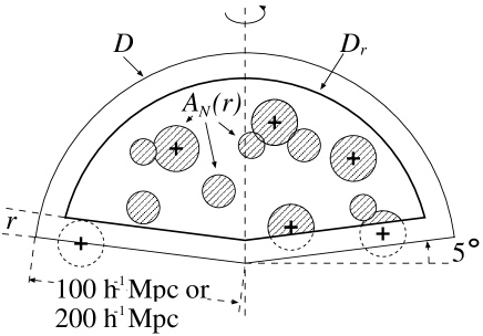
Figure 11: A cut through the union set of balls ${\mathcal{A}}_{N}(r)$, within the shrunken window $D_{r}$.

A.2 Boundary correction for nearest neighbour statistics

? gives several estimators for $F$ and $G$ applicable to spatial point processes with boundaries. In our work we exclusively use the minus estimators (also called reduced sample estimators) $\widehat{F}$ and $\widehat{G}$.

The definition uses the distance $\rho({\mathbf{y}},X)$ of a point ${\mathbf{y}}$ to the nearest point of the pattern $X=\{{\mathbf{x}}_{i}\}_{i=1}^{N}$,

$$\rho({\mathbf{y}},X):=\min(||{\mathbf{x}}_{i}-{\mathbf{y}}||\leavevmode\nobreak\ |\leavevmode\nobreak\ {\mathbf{x}}_{i}{\in}X\mbox{ and }{\mathbf{x}}_{i}\neq{\mathbf{y}}),$$ (16)

and the distance $\rho({\mathbf{y}},D)$ of a point ${\mathbf{y}}$ to the boundary of the window $D$,

$$\rho({\mathbf{y}},D):=\min(||{\mathbf{z}}-{\mathbf{y}}||\leavevmode\nobreak\ |\leavevmode\nobreak\ {\mathbf{z}}\not\in{D}).$$ (17)

As explained in Sect. 2.2, $F(r)$ gives the probability of finding a point of the pattern $X$ within a distance $r$ around a randomly selected point ${\mathbf{y}}$. Therefore we estimate the proportion of points ${\mathbf{y}}\in{D}$ with $\rho({\mathbf{y}},X)\leq{r}$. In order to obtain an unbiased estimator, ${\mathbf{y}}$ has to keep a distance of at least $r$ from the window’s boundary, i.e.  $r\leq\rho({\mathbf{y}},D)$. Therefore, let $\{{\mathbf{y}}_{j}\}_{j=1}^{M}$ be $M$ randomly distributed points ${\mathbf{y}}_{j}\in{D_{r}}$ inside the shrunken window $D_{r}$. Then $\widehat{F}(r)$ is defined by

$$\widehat{F}(r)=\frac{\#\{{\mathbf{y}}_{j}\leavevmode\nobreak\ |\leavevmode\nobreak\ \rho({\mathbf{y}}_{j},X)\leq{r})\}}{M},$$ (18)

where $\#\{\ldots\}$ gives the number of points in the set $\{\ldots\}$.

Note that Eq. (18) is nothing but a Monte Carlo integration of the volume ${\mathcal{A}}_{N}(r)\cap D_{r}$. This is a direct consequence of the equality $F_{0}(r)=m_{0}(r)$ mentioned earlier.

To estimate $G(r)$ we also use a reduced sample estimator Ripley (1988). Since $G(r)$ gives the probability of finding another point of the pattern $X$ within a distance $r$ around a point ${\mathbf{x}}\in{X}$, we simply replace the random sample used in Eq. (18) by the pattern $X$. The minus estimator $\widehat{G}(r)$ is then defined by

$$\widehat{G}(r)=\frac{\#\{{\mathbf{x}}_{j}\leavevmode\nobreak\ |\leavevmode\nobreak\ \rho({\mathbf{x}}_{j},X)\leq{r}\leq\rho({\mathbf{x}}_{j},D)\}}{\#\{{\mathbf{x}}_{j}\leavevmode\nobreak\ |\leavevmode\nobreak\ r\leq\rho({\mathbf{x}}_{j},D)\}}.$$ (19)

A.3 Boundary correction for galaxy count fluctuations

For estimating $\sigma^{2}(r)$ as defined in Eq. (6), we randomly throw two million balls ${\mathcal{B}}_{r}$, count the number of points in each and calculate the variance. In order to take care of the boundaries we only choose balls lying completely within the window $D$. This means their centres have to fall into the shrunken window $D_{r}$.

Appendix B $\sigma^{2}$ for a fractal, and dependence on $\overline{n}$

Figure 10 reveals differences of $\sigma^{2}$ between the 100$h^{-1}$Mpc and the 200$h^{-1}$Mpc samples. Although some of the results are still consistent given the relatively large errorbars, another explanation of the differences is possible. In this appendix we calculate the dependence of $\sigma^{2}$ on the depth $R_{0}$ and the number of points $N_{0}$ for a sample drawn from a fractal distribution of galaxies.

The generalization of $\sigma^{2}$ to point processes on fractal sets is not straightforward, since the mean number density $\overline{n}$ is not well–defined. In the definition given in Eq. (6) we have to replace the number of points in a ball of radius $r$ by $N(r)$ instead of $\overline{n}V({\mathcal{B}}_{r})$, so

$$\sigma^{2}(r):=\frac{\left\langle(N_{i}-N(r))^{2}\right\rangle-N(r)}{N^{2}(r)}$$ (20)

For a fractal of correlation dimension $D$ this quantity depends on the radius through

$$N(r)=\left(\frac{N_{0}}{R_{0}^{D}}\right)r^{D},$$ (21)

where the constant of normalization $N_{0}/R_{0}^{D}$ is given for a spherical sample of radius $R_{0}$ containing $N_{0}$ galaxies. The generalization to cones and an application to number counts is discussed in ?. With Eq. (21) plugged into the definition in Eq. (20) we obtain

$$\sigma^{2}(r)=\frac{\left\langle{N_{i}^{2}}\right\rangle}{N_{0}^{2}}\left(\frac{R_{0}}{r}\right)^{2D}-\frac{1}{N_{0}}\left(\frac{R_{0}}{r}\right)^{D}-1.$$ (22)

Obviously $\sigma^{2}$ depends on $N_{0}$ and $R_{0}$ nontrivially if $D<3$. For a stationary process with $D=3$ the average density $\overline{n}:=N_{0}/V_{0}=N_{0}/(\frac{4\pi}{3}R_{0}^{3})$ is independent of the sample size and we have

$$\sigma^{2}(r)=\left\langle{N_{i}^{2}}\right\rangle(\overline{n}\textstyle\frac{4\pi}{3}r^{3})^{-2}-(\overline{n}\textstyle\frac{4\pi}{3}r^{3})^{-1}-1$$ (23)

as a function of the mean number density $\overline{n}$. Since $\langle\cdot\rangle$ is defined as a volume average, $\left\langle{N_{i}^{2}}\right\rangle$ determined for one realization may differ from an average over several realizations, i.e. universes. If one assumes ergodicity of the point distribution (implying homogeneity), the volume average converges towards the ensemble average. In this case we get for example for a Poisson process $\left\langle{N_{i}^{2}}\right\rangle=(\overline{n}\textstyle\frac{4\pi}{3}r^{3})^{2}+\overline{n}\textstyle\frac{4\pi}{3}r^{3}$ and hence $\sigma^{2}(r)=0$.

References

- Bouchet et al. (1993) Bouchet F. R., Strauss M. A., Davis M. et al., 1993, ApJ 417, 36
- Coleman and Pietronero (1992) Coleman P. H., Pietronero L., 1992, Physics Rep. 213, 311
- Davis (1996) Davis M.: 1996, Is the Universe homogeneous on large scales?. In: Critical Dialogues in Cosmology, Turok, N. (ed.), astro-ph/9610149
- Fava and Santaló (1978) Fava N. A., Santaló L. A., 1978, J. Appl. Prob. 15, 494
- Fava and Santaló (1979) Fava N. A., Santaló L. A., 1979, Z. Wahrscheinlichkeitstheorie verw. Gebiete 50, 85
- Fisher et al. (1994) Fisher K. B., Davis M., Strauss M. A. et al., 1994, MNRAS 266, 50
- Fisher et al. (1995) Fisher K. B., Huchra J. P., Strauss M. A. et al., 1995, ApJS 100, 69
- Hadwiger (1957) Hadwiger H., 1957, Vorlesungen über Inhalt, Oberfläche und Isoperimetrie, Springer Verlag, Berlin
- Kaiser et al. (1991) Kaiser N., Efstathiou G., Ellis R. et al., 1991, MNRAS 252, 1
- Kerscher et al. (1996) Kerscher M., Schmalzing J., Buchert T., Wagner H.: 1996, The significance of the fluctuations in the IRAS 1.2 Jy galaxy catalogue. In: Proc. SFB workshop on Astro–particle physics Ringberg 1996, Report SFB375/P002 (Ringberg, Tegernsee), Bender, R., Buchert, T., Schneider, P. (eds.), p. 83
- Kerscher et al. (1997) Kerscher M., Schmalzing J., Retzlaff J. et al., 1997, MNRAS 284, 73
- Kolatt et al. (1996) Kolatt T., Dekel A., Ganon G., Willick J. A., 1996, ApJ 458, 419
- Lonsdale et al. (1990) Lonsdale C. J., Hacking P. B., Conrow T. P., Rowan-Robinson M., 1990, ApJ 358, 60
- Mann et al. (1996) Mann R. G., Saunders W., Taylor A. N., 1996, MNRAS 279, 636
- Mecke and Wagner (1991) Mecke K. R., Wagner H., 1991, J. Stat. Phys. 64, 843
- Mecke et al. (1994) Mecke K. R., Buchert T., Wagner H., 1994, A&A 288, 697
- Oliver et al. (1996) Oliver S. J., Rowan-Robinson M., Broadhurst T. J. et al., 1996, MNRAS 280, 673
- Peebles (1993) Peebles P. J. E., 1993, Principles of physical cosmology, Princeton University Press, Princeton, New Jersey
- Pietronero et al. (1996) Pietronero L., Montuori M., Sylos Labini F.: 1996, On the fractal structure of the visible Universe. In: Critical Dialogues in Cosmology, Turok, N. (ed.), astro-ph/9611197
- Protogeros and Weinberg (1997) Protogeros Z. A. M., Weinberg D. H., 1997, ApJ 489, 457
- Ripley (1988) Ripley B. D., 1988, Statistical inference for spatial processes, Cambridge University Press, Cambridge
- Rowan-Robinson et al. (1986) Rowan-Robinson M., Walker D., Chester T. et al., 1986, MNRAS 219, 273
- Schmalzing et al. (1996) Schmalzing J., Kerscher M., Buchert T.: 1996, Minkowski functionals in cosmology. In: Proceedings of the international school of physics Enrico Fermi. Course CXXXII: Dark matter in the Universe (Varenna sul Lago di Como), Bonometto, S., Primack, J., Provenzale, A. (eds.), Società Italiana di Fisica, p. 281
- Sylos Labini et al. (1996) Sylos Labini F., Gabrielli A., Montuori M., Pietronero L., 1996, Physica A 226, 195
- Sylos Labini et al. (1997) Sylos Labini F., Pietronero L., Montuori M.: 1997, Frequently asked questions about fractals. In: Proc. SFB workshop on Astro–particle physics Ringberg 1996, Report SFB375/P002 (Ringberg, Tegernsee), Bender, R., Buchert, T., Schneider, P. (eds.), p. 109
- van Lieshout and Baddeley (1996) van Lieshout M. N. M., Baddeley A. J., 1996, Statist. Neerlandica 50, 344
- White (1979) White S. D. M., 1979, MNRAS 186, 145
- Yess et al. (1997) Yess C., Shandarin S. F., Fisher K. B., 1997, ApJ 474, 553