Non-linear Dynamics and Mass Function of Cosmic Structures: I Analytical Results

Abstract

We investigate some modifications to the Press & Schechter (1974) (PS) prescription resulting from shear and tidal effects. These modifications rely on more realistic treatments of the collapse process than the standard approach based on the spherical model.

First, we show that the mass function resulting from a new approximate Lagrangian dynamic ([Audit & Alimi 1996]), contains more objects at high mass, than the classical PS mass function and is well fitted by a PS-like function with a threshold density of $\delta_{c}\simeq 1.4$. However, such a Lagrangian description can underestimate the epoch of structure formation since it defines it as the collapse of the first principal axis. We therefore suggest some analytical prescriptions, for computing the collapse time along the second and third principal axes, and we deduce the corresponding mass functions. The collapse along the third axis is delayed by the shear and the number of objects of high mass then decreases.

Finally, we show that the shear also strongly affects the formation of low-mass halos. This dynamical effect implies a modification of the low-mass slope of the mass function and allows the reproduction of the observed luminosity function of field galaxies. In a companion paper, we present results of numerical simulations which complete this work.

1 INTRODUCTION.

One of the simplest statistical indicators which characterizes the mass distribution in the universe is the mass function of cosmic structures. Press and Schechter (1974, hereafter PS), have proposed a formalism to evaluate this function at any time. For a given hierarchical scenario of structure formation, as for instance CDM, the mass function is obtained using only the power spectrum of the initial density fluctuations. This formalism has been extensively tested with the help of numerical simulations. The first comparison between the mass function of dark-matter halos obtained in numerical simulations and that predicted in the framework of the PS approach have shown a satisfactory agreement ([Efstatiou et al. 1988]). This agreement was later improved by imposing some ad–hoc modifications to the initial PS formalism ([Efstatiou & Rees 1988], [Calberg & Couchman 1989], [Lacey & Cole 1994]). For example, it was shown in these studies that the concordance between the numerical and the analytical predictions was improved by lowering the initial density threshold at which a spherical homogeneous region collapses. However, the theoretical reasons for which a quantity resulting from very non–linear dynamics, such as the mass function, can be computed from this formalism have never been clarified. This question takes on a greater importance because the PS formalism which is a powerful tool, is widely used in phenomenological analytical cosmology. It is, for example, very often used to put constraints on the cosmological parameters using either the luminosity function of galaxies ([White & Frenk 1991], [Blanchard et al. 1992]), the temperature distribution of X-ray clusters ([Oukbir & Blanchard 1992], [Viana & Liddle 1996]) or the Sunayev-Zel’dovich effect ([Cole & Kaiser 1988], [Barbosa et al. 1996], [Eke et al. 1996] and references therein).

The mass function of cosmic structures obtained in the framework of the PS formalism has a statistical and dynamical origin. Starting with the statistical properties of the initial density field, PS identify the fraction of mass embedded in collapsed objects of mass greater than a given mass M, with the fraction of volume filled with regions of space satisfying a given dynamical criterion. Usually the criterion is simply issued from the spherical collapse which selects all the points whose initial density is above a certain threshold. It is highly probable that such a simple model is unable to describe the complex features occurring during a fully non–linear dynamical process. Therefore, one can imagine that only a fraction of regions with a given density contrast exceeding the threshold eventually collapses. This “fuzzy” density criterion can be viewed as a statistical tool ([Blanchard et al. 1992]), but here, in order to have a better understanding of structure formation, we intend to derive it from the gravitational dynamics.

Therefore, in this paper, we study the influence of non-linear dynamics on the mass function, highlighting the role played by shear and tidal effects on the actual shape of the mass function. We present analytical results which exhibit generic features of PS–like mass functions and show the relationship between the dynamics and the mass function through what we call a selection function. Our study concerns both non-spherical Lagrangian dynamical models, and some dynamical “ansatz” that we introduce to describe the structure formation beyond the usual validity range of Lagrangian approximations. In a companion paper we compare our analytical predictions with numerical results.

2 Mass Functions from Lagrangian Dynamics

2.1 PS formalism from a Lagrangian point of view.

The analytical method which has been most successful up to now to compute the mass function is the one introduced by PS. In this paper we use such a formalism but we intend to give our own interpretation of this approach from a Lagrangian point of view (see also [Monaco 1995]). This gives us a general framework for computing the mass function.

The idea of PS is to compute the number density of cosmological objects with mass $M$ at a given time, by identifying the fraction of mass contained in these objects with the mass embedded in the space filled by points with a density which reaches infinity at the same time. When considering an object of mass $M$, the initial density field is smoothed on a scale $R$ with $M\propto R^{3}$. To give a concrete expression for this idea one needs a dynamical prescription that allows to follow the evolution of each point of the initial density field and to know its statistical properties.

Throughout this paper we work in a Friedman-Robertson-Walker universe with a critical density parameter, $\Omega=1$, and initial Gaussian random fluctuations. At some early epoch, corresponding to an expansion factor $a_{i}$ and a redshift $z_{i}$, the density fluctuations are entirely described by their power spectrum. We first multiply this spectrum with a low-pass filter of characteristic scale $R$ that cuts the power above a frequency $\simeq 2\pi/R$. The choice of filter is, a priori, arbitrary ([Lacey & Cole 1994]). We restrict ourselves to the Top–Hat window function in real space, because its application has an intuitive physical interpretation. It allows to consider homogeneous and spherical regions of space. We then assume that the resulting density field is correctly described by independent fluid elements. Each fluid element is now initially described by some dynamical parameters, which are obtained by smoothing the corresponding fields to the scale $R$. Given these initial conditions, we evolve each fluid element separately until it collapses (i.e. until the density of the fluid element becomes infinite). The evolution has to be followed in a Lagrangian way in order to relate the collapse epoch of the fluid element to its initial conditions. In the standard PS approach, these fluid elements evolve according to the homogeneous spherical model. In this case, the collapse epoch is entirely determined by the initial density contrast of the fluid element. However, it has been shown by several authors (e.g. [Van de Weygaert & Babul 1994], [Audit & Alimi 1996]) that, during the gravitational collapse, the shear and the tidal forces are very important. Consequently, more complex, non-spherical, gravitational dynamics have to be considered in order to take into consideration these physical effects which are totally discarded in the spherical model.

For Lagrangian non-spherical dynamics, the collapse time $a_{c}$ of a fluid element can depend on several initial smoothed parameters $x^{j}$, $j=1,n$. The fraction of mass embedded at present ($a=1$) in collapsed structures with a mass greater or equal to $M$ is then given by

$$F(\geq M)=\int P_{R}\left(x^{j}\right)s\left(x^{j}\right)dx^{1}\cdot\cdot\cdot dx^{n}$$ (1)

where $s=1$ if $a_{c}\left(x^{j}\right)\leq 1$ and $0$ otherwise. The selection function $s$ makes a direct link between the Lagrangian dynamics of the fluid elements and the mass function. The integral of $s$, with respect to all $x_{j}$ parameters except the initial density contrast, can be interpreted as a statistical quantity. This quantity gives the probability that a given region of space becomes part of a bound structure according to its initial density contrast ([Blanchard et al. 1992]). The right-hand side of equation (1) depends on $M$ through the smoothing scale $R$. $P_{R}$ is the probability density function of the initial smoothed parameters, it represents the fraction of volume filled by the regions of space having initial parameters $(x^{j}$, $j=1,n)$.

In general, the above definition runs into the so called “renormalization problem”, i.e. $F(\geq 0)=F_{0}\neq 1$. This problem can be alleviated if one carefully considers the fate of regions which have not been selected on a scale $R$, but can be selected with a non–zero probability on another scale $R^{\prime}>R$, and therefore belong to objects with a mass greater than $M$. Excursion set theory ([Peacock & Heavens 1990], [Bond et al. 1991a], 1991b) solves this renormalization problem for the particular case of the sharp-k filter, but the physical interpretation of this filter remains unclear. In this work we do not investigate this renormalization problem. We always assume that this renormalization is justified in any case. We therefore divide the mass fraction obtained in equation (1) by the constant $F_{0}$. The mass function of collapsed objects, which gives the number density of object with mass $M$, is then defined as

$$\Phi(M)=-\frac{\rho_{0}}{M}\frac{d}{dM}\left(\frac{F(>M)}{F_{0}}\right)$$ (2)

In order to determine the mass function we therefore have to evaluate the statistical properties of the initial parameters and the collapse epoch associated with these parameters. In particular, we evaluate the collapse epoch using three different Lagrangian dynamics: the spherical model; the Zel’dovich approximation and a more realistic local Lagrangian model that we introduced in a former paper ([Audit & Alimi 1996]). These three dynamical models state that the fluid element belongs to a collapsed object when its density becomes infinite. For the two latter cases, this first singularity corresponds to the collapse of the fluid element along its first principal axis and then favors the formation of sheet–like objects. One can then ask whether such objects agree with the idea of having a dense, virialized “blob” in the density field. Unfortunately, Lagrangian theory is unable to bypass this first singularity. We therefore investigate two other models in section 3 which roughly describe the collapse of the fluid element along its second and third axis. This comparative analysis of the different mass functions we obtain for each case allows one to study the effect of the dynamics, and in particular, the influence of the shear and the tide on the formation of structures in a PS formalism.

2.2 Computation of the Collapse Epoch

In the simplest cases, only one initial parameter is needed to determine the collapse epoch of a fluid element. This is the case for the spherical model, where the initial density contrast entirely determines the evolution of a fluid element, and for the Zel’dovich approximation where the smallest eigenvalue of the deformation tensor gives the collapse epoch. However, these dynamics are rather simple. It does not seem very realistic to account for the variety of physical processes occurring during the collapse with a single initial parameter. Therefore, we also use a local Lagrangian dynamic which takes into account, to some extend, the effect of the shear and the tide ([Audit & Alimi 1996]), and then determines the collapse epoch in terms of the three eigenvalues of the deformation tensor.

The collapse epoch (written here as the collapse redshift $z_{c}$) of a fluid element evolving according to the spherical model is given by the simple formula

$$1+z_{c}=\frac{\delta}{\delta_{c}}$$ (3)

where $\delta_{c}=\frac{3}{5}(\frac{3\pi}{2})^{2/3}\simeq 1.686$. We use for all fields its initial value linearly extrapolated to $z=0$ (for example: $\delta=(1+z_{i})\delta(z_{i})$). Within the spherical model , the collapse epoch depends only on the initial density contrast and only fluid elements which are initially over-dense, collapse.

In the framework of the Zel’dovich approximation ([Zeldovich 1970]) the density contrast of a fluid element evolves according to

$$1+\delta(t)=\frac{1}{(1+a(t)\lambda_{1})(1+a(t)\lambda_{2})(1+a(t)\lambda_{3})}$$ (4)

where $\lambda_{1}$, $\lambda_{2}$ and $\lambda_{3}$ are the three initial eigenvalues of the deformation tensor arranged in decreasing order. The collapse epoch of the first principal axis is reached when the denominator in equation (4) vanishes

$$1+z_{c}=-\lambda_{3}=\frac{\delta}{3}-\sigma_{3}$$ (5)

Once again $\delta$ is the initial density contrast of the fluid element and $\sigma_{i}$ are its initial shear eigenvalues. In the case of zero shear, the collapse epoch is given by: $1+z_{c}=\delta/3$. This means that the exact solution of the spherical case is not recovered, as can be expected for this first order dynamical prescription. For a fixed density contrast, the shear accelerates the collapse ($\sigma_{3}\leq 0$) and equation (5) can be considered as a first simple approximation for non-spherical dynamics.

The Zel’dovich approximation illustrates in a simple way that the collapse epoch cannot be considered as a function of the density contrast alone. However, computing the collapse epoch in terms of $\lambda_{3}$ alone is not satisfactory either. Therefore, we present in this paragraph a derivation of the collapse time which uses a Lagrangian dynamic based on the deformation tensor. Audit & Alimi (1996), hereafter AA, have proposed a local Lagrangian dynamic to determine the evolution of the eigenvalues of the deformation tensor. Knowing these eigenvalues and their time derivatives is enough to compute all the other dynamical quantities. The dynamical prescription of AA is well suited to the computation of the collapse epoch. It accounts well for the effect of the shear on the collapsing fluid element. It is exact for spherical, cylindrical and planar geometry and very accurate over a wide range of initial conditions. Similar to the Zel’dovich approximation, it predicts that under-dense regions can collapse due to the effect of the shear.

In terms of the eigenvalues of the deformation tensor, the density contrast is defined as

$$1+\delta(\tau)=\frac{1}{\left(1+\lambda_{1}(\tau)\right)\left(1+\lambda_{2}(\tau)\right)\left(1+\lambda_{3}(\tau)\right)}$$

The evolution equation for each of the $\lambda_{i}(\tau)$ is given in the framework of the AA approximation by

$$\frac{d^{2}\lambda_{i}}{d\tau^{2}}=\left(\frac{1+\lambda_{j}/2+\lambda_{k}/2+\lambda_{j}\lambda_{k}/2}{1+\lambda_{j}+\lambda_{k}+\lambda_{j}\lambda_{k}}\right)\frac{6\lambda_{i}}{\tau^{2}}$$ (6)

where $\tau$ is the conformal time defined by: $d\tau=dt/a^{2}$ and $(i,j,k)$ is a circular permutation of $(1,2,3)$. These three equations are highly non linear and have been integrated numerically.

The initial eigenvalues of the shear and deformation tensors are related by: $\lambda_{i}=\sigma_{i}-\delta/3$. The two triplets $(\lambda_{1},\lambda_{2},\lambda_{3})$ and $(\delta,\sigma_{2},\sigma_{3})$ are therefore totally equivalent ($\sigma_{1}$ is obtained using the relation: $\sigma_{1}+\sigma_{2}+\sigma_{3}=0$). In the following, we prefer to use the triplet $(\delta,\sigma_{2},\sigma_{3})$, which allows an immediate physical interpretation. The eigenvalues of the shear and deformation tensor are always arranged in decreasing order: $\sigma_{1}\geq\sigma_{2}\geq\sigma_{3}$ and $\lambda_{1}\geq\lambda_{2}\geq\lambda_{3}$.

Moreover, in order to integrate equation (6) we only keep the linear growing mode in the initial conditions. This restriction and the invariance of equation (6) under the transformation: $\tau\rightarrow\alpha\tau$ ensures the following scaling law for the collapse epoch

$$a_{c}(\delta,\sigma_{2},\sigma_{3})=\alpha a_{c}(\alpha\delta,\alpha\sigma_{2},\alpha\sigma_{3})$$ (7)

Such a property of the collapse time is also present for the spherical model and the Zel’dovich approximation. It allows to reduce by one dimension the parameter space that we have to explore to determine the collapse epoch for any initial condition. It is therefore sufficient to know the function ${\cal T}^{+}(\sigma_{2},\sigma_{3})$ (resp. ${\cal T}^{-}(\sigma_{2},\sigma_{3})$) representing the inverse of the collapse epoch ($a_{c}^{-1}=1+z_{c}$) in the $(\sigma_{2},\sigma_{3})$ plane for $\delta=+1$ (resp. $\delta=-1$). Then, we can deduce the collapse epoch for any set of initial conditions using the scaling law of equation (7). In figure (1), we plot the iso-contours of the functions ${\cal T}^{+}$ and ${\cal T}^{-}$. From the previously given relations between the $\sigma_{i}$ it is easy to deduce that $\sigma_{3}\leq\sigma_{2}\leq-\sigma_{3}/2$. This explains why only a portion of the $(\sigma_{2},\sigma_{3})$ plane is covered. For each of these plots, a thousand points were computed by numerically solving equation (6). We present an analytical fit (accurate to within $1\%$) of these two surfaces in Appendix A. For $\delta>0$, the fluid element always collapses in a finite time. For $\delta<0$, a finite area of shear values is singular (i.e. the collapse time is infinite). This area corresponds to a fluid element whose initial deformation tensor has three positive eigenvalues (all fluid elements with at least one negative eigenvalue collapse).

The two lower panels of figure [1] show the inverse of the collapse time as a function of $\sigma_{3}$ for $\delta=+1$ and $\delta=-1$. The long–dashed line corresponds to the spherical model for which the collapse time is independent of $\sigma_{3}$. The small–dashed line corresponds to the Zel’dovich approximation. The full lines represent the inverse collapse time of the AA dynamics. The upper line corresponds to the case where $\sigma_{2}=\sigma_{3}$ (the fastest collapse at given $\sigma_{3}$ and $\delta$) and the lower line to $\sigma_{2}=-\sigma_{3}/2$ (the slowest collapse at given $\sigma_{3}$ and $\delta$). For $\delta<0$ the collapse time becomes infinite as $\sigma_{3}$ reaches $\delta/3$. The spread between the two full lines gives an idea of the influence of $\sigma_{2}$ on the dynamics and of the importance of the coupling between the different directions of collapse of the fluid element. Note however that the error one could make by neglecting the influence of $\sigma_{2}$ to compute the collapse epoch of the first principal axis is of the order of 20%.

Figure 1: Upper panels: Iso-contours of the redshift of collapse in the ($\sigma_{3},~{}\sigma_{2}$) plane for $\delta=+1$ and $\delta=-1$. The shaded area corresponds to fluid elements which never collapse. Lower panels: The collapse redshift (or the inverse of the collapse epoch) as a function of the smallest eigenvalue of the shear. The solid curves correspond to the two boundary lines of the triangles plotted in the upper graphs. The small-dashed lines correspond to the Zel’dovich approximation. For $\delta=+1$ the spherical model is shown as a long-dashed line.

2.3 Statistics of the Initial Parameters

In the case of initial Gaussian density fluctuations and assuming an initial linear growth mode only, Doroskevitch (1970) derived the probability function for the eigenvalues of the deformation tensor, namely

$$P(\lambda_{1},\lambda_{2},\lambda_{3})=\frac{675\sqrt{5}}{8\pi\Delta^{6}}e^{-\frac{3s_{1}^{2}}{\Delta^{2}}+\frac{15s_{2}}{2\Delta^{2}}}$$

$$\hskip 71.13188pt\times(\lambda_{1}-\lambda_{2})(\lambda_{1}-\lambda_{3})(\lambda_{2}-\lambda_{3})$$ (8)

where $\Delta$ is the r.m.s density contrast smoothed at scale $R$

$$\Delta^{2}(R)=\int 4\pi k^{2}P(k)W^{2}(kR)dk$$ (9)

and $s_{1}=\lambda_{1}+\lambda_{2}+\lambda_{3}$ and $s_{2}=\lambda_{1}\lambda_{2}+\lambda_{2}\lambda_{3}+\lambda_{1}\lambda_{3}$. The $\lambda$’s are correlated variables, $\delta$ and the doublet $(\sigma_{2},\sigma_{3})$ are independent. The probability distribution for these new variables can then be deduced easily from equation (8)

$$P(\delta,\sigma_{2},\sigma_{3})=\frac{1}{\Delta^{3}}P_{\nu}\left(\frac{\delta}{\Delta}\right)P_{\mu_{2},\mu_{3}}\left(\frac{\sigma_{2}}{\Delta},\frac{\sigma_{3}}{\Delta}\right)$$ (10)

where the marginal probability functions for the rescaled variables $\nu=\delta/\Delta$ and $\mu_{i}=\sigma_{i}/\Delta$ are given by

$$P_{\nu}=\frac{1}{\sqrt{2\pi}}e^{-\nu^{2}/2}$$ (11)

and

$$P_{\mu_{2},\mu_{3}}=\frac{675}{4}\sqrt{\frac{5}{2\pi}}e^{-7.5(\mu_{2}^{2}+\mu_{2}\mu_{3}+\mu_{3}^{2})}$$

$$\hskip 56.9055pt\times(\mu_{2}+2\mu_{3})(\mu_{3}+2\mu_{2})(\mu_{2}-\mu_{3})$$

We compute also the marginal probability distribution functions of $\mu_{1}\in[0,+\infty[$ and $\mu_{3}\in]-\infty,0]$

$$P_{\mu_{1}}=P_{\mu_{3}}=3\sqrt{\frac{5}{2\pi}}e^{-45\mu_{3}^{2}/8}$$ (12)

$$\hskip 56.9055pt\times\left(e^{-135\mu_{3}^{2}/8}-(1-\frac{135}{8}\mu_{3}^{2})\right)$$

and of $\mu_{2}\in]-\infty,+\infty[$

$$P_{\mu_{2}}=3\sqrt{\frac{5}{2\pi}}e^{-45\mu_{2}^{2}/2}$$ (13)

Equation (1) can be now re-written in terms of $\nu$, $\mu_{2}$, $\mu_{3}$ and $\Delta$.

$$\!\!\!\!\!\!F(\geq M)=\!\!\int\!\!P_{\nu}P_{\mu_{2},\mu_{3}}s(\nu\Delta,\mu_{2}\Delta,\mu_{3}\Delta)d\nu d\mu_{2}d\mu_{3}$$ (14)

The only quantity which then depends on $M$ is $\Delta$. Consequently, the mass function can be expressed as

$$\Phi(M) = -\frac{\rho_{0}}{M}\frac{d\Delta}{dM}\frac{1}{F_{0}}$$ (15)

$$\times \int P_{\nu}P_{\mu_{2},\mu_{3}}\frac{\partial s}{\partial\Delta}(\nu\Delta,\mu_{2}\Delta,\mu_{3}\Delta)d\nu d\mu_{2}d\mu_{3}$$

where the integral is a function of $\Delta$ and depends only on the chosen dynamics which gives its specific form to $s$. It is therefore possible to define a universal mass function for each dynamic which is independent of the initial power spectrum of the density fluctuation. The mass function can be written, for any spectrum, in the form

$$\Phi(M)=-\frac{\rho_{0}}{M}\frac{d\Delta}{dM}\Phi(\Delta)$$ (16)

The spectrum dependence of the mass function is totally contained in the $d\Delta/dM$ factor. We call $\Phi(\Delta)$, which depends only on the chosen dynamics (i.e. on the function $1+z_{c}$), the universal mass function. This demonstrates that the mass function resulting from a PS formalism admits, in addition to the well know time self-similarity, a “scaling” behavior in spectrum (see also [Lacey & Cole 1994]). This property holds only in a critical universe, independently of the dynamics as long as only the growing mode is kept during the linear regime. These two “scaling properties” of the mass function are general characteristics of a PS–like mass function. Therefore, they can be used as test for the validity of a PS approach to the mass function.

2.4 Mass Functions

Equation (1) can now be re-written as follows

$$F(\geq M)=\frac{1}{\sqrt{2\pi}}\int_{-\infty}^{+\infty}e^{-\nu^{2}/2}S(\nu\Delta,\Delta)d\nu$$ (17)

For the spherical model, $S$ is identical to the selection function $s$ which depends then only on the initial density contrast

$$s(\nu\Delta)=\left\{\begin{array}[]{l}0\mbox{ if }\nu\Delta<\delta_{c}\\ 1\mbox{ otherwise }\\ \end{array}\right.$$ (18)

For the Zel’dovich and AA approximations, the selection function is not a function of the density contrast alone. In equation (17), $S$ is then the selection function, integrated over all parameters ($\mu_{3}$ for Zel’dovich approximation and $\mu_{2}$ and $\mu_{3}$ for AA approximation), except $\nu$. For the AA dynamical model, $S$ is explicitly given by

$$\begin{array}[]{ll}S(\nu\Delta,\Delta)=\int_{-\infty}^{0}\int_{\mu_{3}}^{-\mu_{3}/2}&S(\nu\Delta,\mu_{2}\Delta,\mu_{3}\Delta)\\ &\times P_{\mu_{2},\mu_{3}}d\mu_{2}d\mu_{3}\\ \end{array}$$ (19)

It represents the probability that a fluid element with a given initial density contrast, collapses in the age of the Universe. In figure (2), we plot this quantity and its derivative with respect to $\Delta$ for $\Delta$ = 0.5, 1 and 2. A small $\Delta$ value corresponds to high mass objects, and a large $\Delta$ value to small mass objects. One clearly sees that for $\Delta=2$, negative values of the density contrast are selected, showing that shear effects can actually lead to the collapse of under-dense regions. For $\Delta=0.5$, the selection functions become steeper and converge towards an Heavyside function. For the Zel’dovich model, the selection function in the limit $\Delta\rightarrow 0$ leads to a Heavyside step function at $\delta=3$, illustrating that this model is only a first order approximation. For the AA model, the selection function converges in the limit $\Delta\rightarrow 0$ towards the Heavyside function at $\delta=\delta_{c}$. The derivative of the selection function $\partial S/\partial\Delta$ peaks at a value lower than $\delta_{c}$, and this peak value tends towards $\delta_{c}$ as $\Delta\rightarrow 0$. Therefore, in the AA approximation, where objects are defined by the collapse of their first principal axis, the mean initial density contrast is lower than the standard spherical threshold $\delta_{c}$.

Figure 2: Selection functions and their derivatives (see text for definitions) obtained at $\Delta$=2 (dotted line), $\Delta$=1 (solid line) and $\Delta$=0.5 (dashed line) for the Zel’dovich model (two lower graphs) and for the AA model (two upper graphs).

We deduce now the universal mass function

$$\Phi(\Delta)=-\frac{1}{F_{0}}\frac{1}{\sqrt{2\pi}}\int_{-\infty}^{+\infty}e^{-\nu^{2}/2}\frac{\partial S}{\partial\Delta}d\nu$$ (20)

For the spherical dynamics $F_{0}=0.5$ since only 50% of the regions of space collapse (those with a positive density contrast). For the Zel’dovich and AA approximations, $F_{0}\simeq 0.92$ as all regions with a negative $\lambda_{3}$ collapse. In figure (3) we plot $\Phi(\Delta)$ for the three different dynamics. The bottom figure is shown with a linear scale to allow an easy examination of the maximum amplitude of the mass functions. The top one, shown on a logarithmic scale, is better adapted to observing the small mass (high $\Delta$) slope and the high mass (small $\Delta$) cut–off. The mass function computed with our dynamical model (full line) is very well fitted by a standard PS mass function with a critical density parameter $\delta_{c}=1.4$ (short–dashed line). This is easily explained by the behavior of the selection function previously discussed, whose effective threshold is lower than the spherical threshold $\delta_{c}$. On the contrary, for the Zel’dovich approximation, the resulting mass function cannot be approximated by a PS function with another value of $\delta_{c}$. The high–mass cut–off is however located at lower mass, as can be expected from the selection function which chooses regions with an effective threshold higher than the standard value $\delta_{c}$. All mass functions have an exponential cut-off at high mass and a power law behavior at small mass. However, this doesn’t mean that the resulting mass function can always be fitted by the PS formula, with $\delta_{c}$ as fit parameter.

Figure 3: Universal multiplicity functions on linear and logarithmic scales. The solid line corresponds to our dynamical model (Audit & Alimi 1996), the dashed line to the PS mass function with $\delta_{c}=1.4$, the dotted line to the standard PS mass function ($\delta_{c}=1.686$) and the long–dashed line to the Zel’dovich approximation.

Moreover, we see that the standard ($\delta_{c}\simeq 1.686$) PS mass function (dotted line) and our mass function have roughly the same slope for small mass objects, although we predict more high mass objects than the standard PS. For example, if the power spectrum is normalised with the condition $\Delta(R=8Mpc.h^{-1})=1$ and assuming assume a critical Univers with $h=0.5$, we find that our mass function contains $30\%$ more structures of mass $\approx 10^{15}M_{\odot}$, which is the typical mass of galaxy clusters.

3 Beyond Lagrangian Models

In the previous section we have computed the mass function in the framework of the PS formalism using different Lagrangian dynamical models to determine the collapse epoch of a fluid element. In all cases, the collapse was defined as the epoch when the density contrast becomes infinite. It is then impossible to follow, with Lagrangian dynamics, the evolution of a fluid element beyond this first singularity. Moreover, if one considers that the fluid elements describe extended regions of space, this first singularity corresponds to a stage where the region has totally collapsed along a single direction and reached a sheet–like geometry. The resulting “pancakes” may, however, not be the dense virialized halos that one would expect as well defined objects in the density field. It is therefore interesting to investigate what happens when one waits for the collapse of the fluid element along its second or third axis which corresponds to filamentary or quasi-spherical objects respectively. The mass function deduced from the collapse of the third axis will be presented in greater detail, as it is, in our opinion, best suited for dense virialized objects in the density field.

In section 2.3 and figure (1), we have seen that the dispersion of the collapse epoch of the first axis, in the AA approximation, due to the shear on the second axis was of the order of 20%. This weak dependence suggests that, as in the Zel’dovich approximation, the different directions of the fluid element can be considered as collapsing independently. This approximation allows to artificially go beyond the first singularity and to propose an ansatz for the collapse epoch of the second and third axis in order.

We require that the collapse epoch of a fluid element along any of its principal axis satisfies the following properties:

• The collapse epoch along a given axis is a function of the corresponding initial shear eigenvalue and of the initial density contrast.

• The scaling properties (eq. [7]) should be satisfied.

• The spherical collapse epoch should be recovered if the initial eigenvalue of the shear along this direction is zero.

• The collapse epoch should be a monotonically increasing function of the shear. A positive (resp. negative) shear eigenvalue should slow down (resp. accelerate) the collapse relative to the corresponding spherical model.

These properties mean that the following formulae hold

$$a_{c}(\delta,\sigma_{i})=\frac{1}{\delta}a_{c}(1,\sigma_{i}/\delta)=\frac{1}{\delta}\tilde{a}_{c}(\sigma_{i}/\delta)$$ (21)

where $\tilde{a}_{c}$ is a monotonous increasing function and $\tilde{a}_{c}(0)=\delta_{c}$. Since $\tilde{a}_{c}$ is monotonous, it is also bijective and has an inverse, $\tilde{\sigma}_{c}$, which gives the shear corresponding to a given collapse epoch in the $\delta=+1$ plane (note that there are, as in the previous section, two functions $\tilde{a}_{c}$, one for the positive and one for the negative density contrasts).

3.1 Mass Functions of Sheets, Filaments or Knots

In order to push our investigations further we now propose a simple ansatz for the collapse time along each axis. We do not have an underlying dynamical model to justify for the following approximation of the collapse epoch of the different axes. These models are a phenomenological approach to studying qualitatively the influence of considering the collapse along a given axis.

For $\delta>0$ and $\sigma_{i}<0$ as well as for $\delta<0$ we approximate by linear functions the results given in the previous section

$$1+z_{c} = \delta/\delta_{c}-\alpha\sigma_{i}\qquad\mbox{ if }\delta>0\mbox{ and }\sigma_{i}<0$$ (22)

$$1+z_{c} = \alpha(\delta/3-\sigma_{i})\;\;\,\mbox{ if }\delta<0$$ (23)

With this model we recover, for $\delta>0$, the spherical collapse epoch for $\sigma_{i}=0$ and for $\delta<0$. The collapse time becomes infinite for $\sigma_{i}=\delta/3$. The slope $\alpha$ is a free parameter, it has to satisfy $0.8\leq\alpha\leq 1$ in order to recover approximately the right collapse time for the first axis (fig. 4).

Figure 4: The collapse redshift as a function of the eigenvalue of the shear. The ansatz defined by Eqs. (22) and (23) are shown by the full-line for the part deduced from the linear fit of the results of previous section. The dashed-line represents the extrapolation in the $\delta>0,\sigma_{i}>0$ region ($\alpha=0.8,\epsilon=1$) (Eq. 24). As a reminder, the results of the previous section are shown as a dotted-line.

To compute the mass function for any axis, we also need to know the collapse epoch for $\delta>0$ and $\sigma_{i}>0$. Unfortunately, in this case we do not have any dynamical model to determine the function $\tilde{a}_{c}$. However, to study the qualitative behavior of the mass function we choose a simple ansatz for the collapse time given by

$$1+z_{c}=\frac{\delta}{\delta_{c}}(1-\frac{\sigma_{i}}{\sigma_{c}\delta})^{\epsilon}$$ (24)

The spherical collapse time is once again found for vanishing shear The shear totally prevents the fluid element from collapsing when $\sigma_{i}\geq\sigma_{c}\delta$. Note that for large values of $\sigma_{c}$ we find the spherical model everywhere. $\epsilon$ is a positive, free parameter which determines the global shape of the function $\tilde{a}_{c}$. This parameterization is somewhat arbitrary but satisfies the general requirements presented above. We now compute the selection function, its derivative and the universal mass function for objects which collapse along the first, second or third axis.

3.1.1 First axis collapse

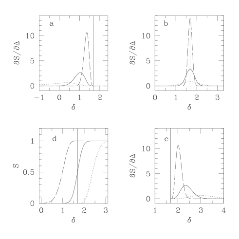
Figure 5: Derivative of the selection function for $\Delta=0.5$, $1$ and $2$ (long-dashed, solid and dotted lines respectively) and for first, second and third axis collapse (fig. a, b and c respectively). Figure d shows the selection function for $\Delta=1$ for the collapse of the first, second and third axes (long-dashed, solid and dotted lines respectively). In all figures the vertical solid line indicates the position $\delta=\delta_{c}$.

This case has been studied in detail in the previous sections. We want to show here that the results are not strongly affected in neglecting the influence of $\sigma_{2}$. Since $\sigma_{3}$ is always negative we use formulae (22) and (23) for the collapse epoch. We have plotted in figure (5) the selection function and its derivative for the case $\alpha=0.8$ and for different values of $\Delta$. The difference with the results of the previous sections is always less than a few percent. As was already mentioned before, the selection function is equal to unity for $\delta>\delta_{c}$ and continuously decreases towards zero when $\delta\rightarrow-\infty$. Its derivative sharpens and peaks at a value which goes towards $\delta_{c}$ (while remaining smaller) as $\Delta$ decreases. The resulting mass function is plotted on figure (6) and always differs by less than 10% to the one obtained in the previous section.

3.1.2 Second Axis Collapse

The collapse epoch of the second axis is a function of $\delta$ and $\sigma_{2}$. In the last section, $\sigma_{3}$ varies between $-\infty$ and $0$. Now, $\sigma_{2}$ belongs to the domain $]-\infty,+\infty[$. Therefore we use for the collapse epoch, the formulae (22), (23) and (24). We have plotted in figure (5) the selection function and its derivative for the case $\alpha=0.8$, $\epsilon=1$ and $\sigma_{c}=1/\alpha\delta_{c}$ (we have just extrapolated formula (22) for the domain $\sigma_{2}>0$). In this case the selection function increases from zero to one when $\delta$ goes from $-\infty$ to $+\infty$ and is equal to one-half for $\delta=\delta_{c}$ (all the points with $\mu_{2}\leq 0$ (50%) which collapse faster than the spherical model are selected). As before, a fraction of the fluid elements with $\delta<\delta_{c}$ are selected, but contrary to what happened in the previous case, a fraction of the fluid elements with $\delta>\delta_{c}$ are unable to collapse because of shear effects. The derivative of the selection function peaks at around $\delta_{c}$ (exactly at $\delta_{c}$ for our model) and has a width which tends towards zero in the limits of vanishing $\Delta$.

The resulting mass function is plotted in figure (6). It is now quite close to the standard PS mass function, which means that the number of objects with $\Delta\lesssim 1$ has considerably decreased compared to the first axis collapse. This fact is not very surprising because in this case, the shear can either slow down the collapse for $\sigma_{2}>0$ or accelerate it for $\sigma_{2}<0$. These two effects roughly cancel each other, and one obtains a quasi–spherical model.

3.1.3 Third Axis Collapse

Figure 6: Mass function obtained for first, second and third axes collapse (dotted, dashed and long-dashed lines). The solid line is the classical ($\delta_{c}=1.686$) Press and Schechter mass function.

We now present in greater detail the mass function obtained for objects that collapse along their third axis. In this case the collapse epoch is a function of $\delta$ and $\sigma_{1}\in[0,+\infty[$. It is possible to derive analytically the selection function, its derivative and the corresponding mass function for a given $\tilde{a}_{c}$. After some algebra, we obtain

$$S_{\tilde{a}_{c}}(\nu\Delta,\Delta)=\int_{0}^{\nu\tilde{\sigma}_{c}(\nu\Delta)}P_{\mu_{1}}d\mu_{1}$$ (25)

Taking the derivative of this equation with respect to $\Delta$ yields

$$\frac{\partial S_{\tilde{a}_{c}}}{\partial\Delta}(\nu\Delta,\Delta)=P_{\mu_{1}}\left(\nu\tilde{\sigma}_{c}(\nu\Delta)\right)\nu^{2}\dot{\tilde{\sigma}}_{c}(\nu\Delta)$$ (26)

where $\dot{\tilde{\sigma}}_{c}$ symbolizes the derivative of the function ${\tilde{\sigma}}_{c}$. Finally, using the variable $x$ defined by $x=\tilde{\sigma}_{c}(\nu\Delta)$, the universal mass function can be expressed as

$$\!\!\!\!\!\!\!\!\Phi(\Delta)=\frac{F_{0}^{-1}}{\sqrt{2\pi}}\int_{0}^{\sigma_{c}}\!\!\!\!e^{-\frac{{\tilde{a}_{c}}^{2}(x)}{2\Delta^{2}}}P_{\mu_{1}}\left(\frac{x\tilde{a}_{c}(x)}{\Delta}\right)\frac{{\tilde{a}_{c}}^{2}(x)}{\Delta^{3}}dx$$ (27)

where $\sigma_{c}\in]0,+\infty]$ is the value of $x$ at which $\tilde{a}_{c}$ becomes infinite. A similar calculation can be carried out for all axes. The above formula is a general relation between the mass function and the collapse time defined by the underlying dynamical model.

For the third axis, we assume that the collapse epoch is now given by equation (24) and we use the same parameters as for the second axis. The selection function (Fig. [5]) tends to zero as $\delta\rightarrow\delta_{c}$ and to unity as $\delta\rightarrow+\infty$. This reflects the fact that a fraction of the fluid elements with $\delta\geq\delta_{c}$ are unable to collapse as the shear inhibits the collapse.

The derivative of the selection function behaves symmetrically about the line $\delta=\delta_{c}$ compared to the one obtained for the first axis. Its derivative sharpens and peaks at a value which tends towards $\delta_{c}$ (while remaining larger) as $\Delta$ decreases. In the class of models with $\epsilon=1$, it is possible to derive an analytical expression for these qualitative features. We compute the mean (which is close to the peak value) and the variance (which corresponds to the width) of the function $\partial S/\partial\Delta$. We obtain for the mean

$$\bar{\delta}=\delta_{c}+\frac{3}{5}\sqrt{\frac{5}{2\pi}}\frac{\Delta}{\sigma_{c}}\simeq\delta_{c}+0.54\frac{\Delta}{\sigma_{c}}$$ (28)

and for the variance

$$\Sigma=\frac{1}{3}\sqrt{\frac{29\pi-81}{10\pi}}\frac{\Delta}{\sigma_{c}}\simeq 0.19\frac{\Delta}{\sigma_{c}}$$ (29)

In these last two equations the width and the peak position are linear functions of $\Delta$. Note also that as $\Delta\rightarrow 0$, we get $\bar{\delta}=\delta_{c}$ and $\Sigma=0$, as in the spherical model.

The mass function can also be derived analytically. Using formula (27), we obtain

$$\Phi(\Delta)=\frac{F_{0}^{-1}}{\sqrt{2\pi}}\frac{\delta_{c}}{\Delta^{2}}\int_{0}^{+\infty}\!\!\!\!e^{-\frac{1}{2}\left(\frac{\delta_{c}}{\Delta}+\frac{\mu}{\sigma_{c}}\right)^{2}}P_{\mu_{1}}(\mu)d\mu$$ (30)

The mass function now has two “dynamical parameters”, namely $\delta_{c}$ and $\sigma_{c}$. The first one describes the influence of the initial density contrast on the collapse epoch and the second one gives the degree of inhibition of the collapse by the shear and the tidal field. The spherical mass function is recovered in the limits $\sigma_{c}\rightarrow+\infty$ and for small values of $\sigma_{c}$ most of the fluid elements are unable to collapse because of shear effects. This mass function for $\sigma_{c}=0.74$ and $\delta_{c}=1.686$ is plotted in figure (6) as a long–dashed line. The number of objects with $\Delta\lesssim 1$ has again greatly decreased compared to the second axis collapse. As could be expected, since now the shear always slows down the collapse, the mass function is now much below the standard PS prediction.

In the next section we investigate the generic behavior of the mass function obtained in this section (Eq. [27]) in the low–mass regime.

3.2 Low Mass Behavior of the Mass Functions

In the previous section, we postulated a specific form for the collapse epoch of a given fluid element, as a function of $\delta$ and the shear along the third axis. In this section, we study in a more general way the influence of the shear on the formation of low mass objects. We consider that the function $\tilde{a}_{c}$ has the following asymptotic behavior when $x\rightarrow\sigma_{c}$

$$\tilde{a}_{c}@>>{\sigma_{c}}>\left(\sigma_{c}-x\right)^{-\epsilon}$$ (31)

where $\epsilon>0$. This parameterization is very general, and makes no assumptions on the general shape of the function $\tilde{a}_{c}$. We calculate analytically the low–mass (high–$\Delta$) behavior of the mass function as a function of $\epsilon$. After some algebra (cf. Appendix B), we obtain two characteristic regimes, valid in the limit $\Delta\gg 1$

$$\Phi \propto\Delta^{-\left(\frac{\epsilon+1}{\epsilon}\right)} \mbox{ if }\epsilon\geq\frac{1}{6}$$ (32)

$$\Phi \propto\Delta^{-7} \mbox{ if }\epsilon\leq\frac{1}{6}$$ (33)

Note that for the case $\epsilon=1$, the low–mass behavior is the same as for the standard Press & Schechter mass function. The domain $\epsilon>1$ corresponds to shallower slopes than the standard PS mass function. However, the Zel’dovich approximation corresponds to $\epsilon=1$. Therefore, if one considers that this first order approximation overestimates the collapse time, this imposes that

$$0<\epsilon<1$$ (34)

We plot in figure (7) the mass functions we obtained using the collapse epoch from formula (24) for different values of $\epsilon\leq 1$. We set the parameter $\sigma_{c}=3$ for each curve in figure (7). This parameter determines the point where the change of slope occurs in the mass function (in our case, this corresponds to $\Delta\simeq 5$).

This result is extremely important as it shows that shear effects can easily modify the low–mass behavior of the mass function. The regime $\epsilon\leq 1/6$ is of primary importance, because it is independent of the specific form of the function $\tilde{a}_{c}$, which is unfortunately an unknown quantity. In this case, for a power law power spectrum, one obtains in the low–mass end of the mass function $\Phi(M)\propto M^{n+1}$ where $n$ is the index of the power spectrum. Assuming a constant mass–to–light ratio, this leads to a faint–end slope of the luminosity function $\alpha=n+1$. Note that the corresponding power law for the standard PS mass function would have been $\alpha=-2+(n+3)/6$. The observed luminosity function of field galaxies exhibits this power law behavior at low–luminosity with $\alpha\simeq-1$ (Loveday et al. 1994; Efstathiou, Ellis & Peterson 1988). It has been previously argued (Blanchard et al. 1992) that for a CDM power spectrum with $n\simeq-2$ at these scales, it is impossible to reconcile the PS formalism ($\alpha\simeq-1.83$) with the observed luminosity function without imposing some ad–hoc procedures, such as a variable mass–to–light ratio, or some other biasing mechanism due to the dissipative physics of the baryonic gas. Here, we recover $\alpha\simeq-1$ with a power spectrum $n\simeq-2$, using only gravitational processes, and more precisely by considering the effect of the shear. We claim here that the a CDM–like power spectrum is able to reproduce the low–mass end of the luminosity function, when the shear and tidal effects are correctly taken into account. Note that the PS formalism is better suited for field galaxies than for galaxies in clusters where tidal effects are much stronger. With this formalism, the clusters are considered as single objects whose internal structure can not be described.

Figure 7: Mass function obtained for the third axis collapse and for $\epsilon$=1, 1/2, 1/4, 1/6 and 1/100 (solid, dotted, dashed, long-dashed and dotted-dashed lines respectively). Note that for $\epsilon\leq 1/6$ the slope at low mass remains equal to $-7$.

4 Conclusion

In this paper, we extend the PS formalism to more complex, and perhaps more realistic dynamical models than the standard spherical model. We study the influence of the shear and tidal effects on the mass function of cosmic structures.

The Lagrangian evolution of a given halo from the initial volume up to the final dense and virialized object, can be divided into three stages: the collapse of the first, second and third axes. Each stage corresponds to a certain geometry of the halo formed (sheet–like, filamentary and quasi–spherical) and also to a certain collapse epoch. In the Lagrangian formalism, this collapse epoch depends purely on the initial shear and density contrast. The mass function of these halos is then obtained from the collapse epoch and from the statistics of the initial parameters.

We investigate in this paper the influence of the initial shear on the dynamics of the forming halos. In the case of sheet–like objects, the Lagrangian theory of gravitational dynamics allows us to compute the collapse epoch of the first principal axis as a function of $\delta$ and $\sigma_{3}$ and $\sigma_{2}$, the initial density contrast and two eigenvalues of the initial shear tensor. We use for that purpose a new approximation presented by Audit & Alimi (1996). In this case we obtain a mass function which is well fitted by a PS mass function, with $\delta_{c}=1.4$. This result is explained by the fact that shear and tidal effects always accelerate the collapse of a fluid element along its first principal axes. We therefore obtain more high–mass objects than the standard PS mass function (see also Monaco 1995).

We then investigate the mass function of objects that collapse along their second and third principal axis. We considere simple and general models since Lagrangian theory is unable to describe the evolution of a fluid element beyond the collapse of the first axis. We find that the resulting mass function in the case of the second axis collapse is very similar to the standard PS mass function ($\delta_{c}\simeq 1.686$).

Finally, we derive analytically a new formula for the mass function of objects resulting from the collapse of their third axis. This depends on two parameters, namely a density threshold $\delta_{c}$ and a shear threshold $\sigma_{c}$. We recover the standard PS formula in the case $\sigma_{c}\rightarrow+\infty$. For values of $\sigma_{c}$ comparable to unity, the peak of the multiplicity function is lower than the peak obtained by the standard PS approach. This could explain why such an effect has been detected in numerical simulations (Efstathiou et al. 1988). We also derive analytically the low–mass regime of the mass function computed in a wide class of models. We show that it is possible to obtain a low–mass slope very close to the faint–end slope of the luminosity function of field galaxies.

In all the dynamical models we use, the resulting mass functions show common features such as a high–mass exponential cut–off and a low–mass power law. The exact shape of the multiplicity function around the peak is, however, directly related to the underlying dynamical model. This has to be tested in numerical simulations, where the mass function should correspond to a dynamical model that drives the collapse of every halo (at least in a statistical sense). We postpone this numerical work to a companion paper.

Appendix A Collapse Epoch using our Dynamical Model

In this appendix we present the collapse time obtained from the AA dynamics. The following formulae were obtained by fitting a thousand points for $\delta>0$ and $\delta<0$. The fits are accurate to about 1%.

For $\delta>0$, we obtain

$${\cal T}^{+}=1+z_{c}=\frac{x^{3}-1}{7}f^{+}+\frac{8-x^{3}}{7}f^{-}$$

where $x\in[1,2]$ is defined by

$$x=\left(1+\frac{1}{3}\left(1+2\frac{\sigma_{2}}{\sigma_{3}}\right)^{2}\right)^{1/2}$$

The functions $f^{+}$ and $f^{-}$ depend only on $\sigma_{3}/\delta$, and are proportional to $\delta$, according to the scaling property derived in section 2.

$$f^{+}=\delta\left(\frac{1}{\delta_{c}}-\frac{\sigma_{3}}{\delta}-0.2(1-g^{+})\right)$$

$$g^{+}=\left(1-10\sigma_{3}/\delta\right)^{-1/2}$$

$$f^{-}=\delta\left(\frac{1}{\delta_{c}}-0.81\frac{\sigma_{3}}{\delta}-0.18(1-g^{-})\right)$$

$$g^{-}=\left(1-4.5\sigma_{3}/\delta\right)^{-1}$$

Note that the spherical model is recovered for vanishing shear. The Zel’dovich solution, which is exact when $\sigma_{3}=-2\delta/3$ and $\sigma_{2}=-\sigma_{3}/2$, is also recovered.

For $\delta<0$, we have

$${\cal T}^{-}=1+z_{c}=\frac{x^{3a}-1}{8^{a}-1}f^{+}+\frac{8-x^{3a}}{8^{a}-1}f^{-}$$

where $x\in[1,2]$ is the same as for $\delta>0$ and $a$ is given by

$$a=\left(1+\frac{0.5}{3\sigma_{3}/\delta-1}\right)^{1/2}$$

The functions $f^{+}$ and $f^{-}$ are now given by

$$f^{+}=-\delta\left(\left(\frac{\sigma_{3}}{\delta}-\frac{1}{3}\right)-0.2(1-g^{+})\right)$$

$$g^{+}=\left(1+15\left(\sigma_{3}/\delta-1/3\right)\right)^{-1/3}$$

$$f^{-}=-\delta\left(0.81\left(\frac{\sigma_{3}}{\delta}-\frac{1}{3}\right)-0.18(1-g^{-})\right)$$

$$g^{-}=\left(1+4.5\left(\sigma_{3}/\delta-1/3\right)\right)^{-1}$$

When the shear is much larger than the density contrast both ${\cal T}^{+}$ and ${\cal T}^{-}$ converge toward the same value as expected.

Appendix B Computation of the low-mass behavior of the mass function for the third axis collapse

We present in this appendix the derivation of the low-mass behavior presented in section (3.2). From equations (20) and (26) the universal mass function can be written as

$$\Phi(\Delta)\propto\int_{\delta_{c}/\Delta}^{+\infty}e^{-\nu^{2}/2}P_{\mu_{1}}(\nu\tilde{\sigma_{c}}(\nu\Delta))\nu^{2}\dot{\tilde{\sigma_{c}}}(\nu\Delta)d\nu$$ (35)

We want to study the behavior of the previous integral for the case where $\Delta\rightarrow\infty$. The collapse time has the behavior given by equation (31) which allows to calculate the following limits

$$\tilde{\sigma}_{c}(x)@>>{\infty}>\sigma_{c}\>\mbox{ and }\>\dot{\tilde{\sigma}}_{c}(x)@>>{\infty}>\frac{1}{\epsilon}x^{-(\epsilon+1)/\epsilon}$$ (36)

We then divide into two the integral giving the mass function

$$\cal{I}_{1}=\int_{1}^{+\infty}e^{-\nu^{2}/2}P_{\mu_{1}}(\nu\tilde{\sigma_{c}}(\nu\Delta))\nu^{2}\dot{\tilde{\sigma_{c}}}(\nu\Delta)d\nu$$ (37)

$$\cal{I}_{2}=\int_{\delta_{c}/\Delta}^{1}e^{-\nu^{2}/2}P_{\mu_{1}}(\nu\tilde{\sigma_{c}}(\nu\Delta))\nu^{2}\dot{\tilde{\sigma_{c}}}(\nu\Delta)d\nu$$ (38)

Using the limits given above, we have for large values of $\Delta$

$$\cal{I}_{1}\sim\int_{1}^{+\infty}e^{-\nu^{2}/2}P_{\mu_{1}}(\nu\sigma_{c})\nu^{2}\frac{1}{\epsilon}(\nu\Delta)^{-(\epsilon+1)/\epsilon}d\nu$$ (39)

Therefore, the asymptotic behavior of $\cal{I}_{1}$ when $\Delta\rightarrow\infty$ is

$$\cal{I}_{1}\sim\Delta^{-\frac{\epsilon+1}{\epsilon}}$$ (40)

Changing back from $\nu$ to $\delta$ and using the limits given in equations (36), $\cal{I}_{2}$ can be written as

$$\cal{I}_{2} = \int_{\delta_{c}}^{\Delta}e^{-\delta^{2}/2\Delta^{2}}P_{\mu_{1}}(\frac{\delta}{\Delta}\tilde{\sigma_{c}}(\delta))(\frac{\delta}{\Delta})^{2}\dot{\tilde{\sigma_{c}}}(\delta)\frac{d\delta}{\Delta}$$ (41)

$$= \int_{\delta_{c}}^{\Delta}\left(\sum_{n=2}^{\infty}f_{n}\right)d\delta$$ (42)

where $f_{n}=\alpha_{n}\frac{\delta^{2n+1-1/\epsilon}}{\Delta^{2n+3}}$ and $\alpha_{n}$ are numerical constants. ($P_{\mu_{1}}$ and the exponential have been developed in series).

If $\epsilon\geq 1/2(n+1)$, $\int f_{n}d\delta$ diverges and we have

$$\int_{\delta_{c}}^{\Delta}f_{n}d\delta\sim\Delta^{-\frac{\epsilon+1}{\epsilon}}$$ (43)

If $\epsilon<1/2(n+1)\leq 1/6$, $\int f_{n}d\delta$ converges and therefore

$$\int_{\delta_{c}}^{\Delta}f_{n}d\delta\sim\Delta^{-2n+3}\leq\Delta^{-7}$$ (44)

Keeping only the leading terms from equations (40), (43) and (44) gives the asymptotic behavior of $\Phi(\Delta)$ (Eqs. (32) and (33)).

References

- [Audit & Alimi 1996] Audit, A. & Alimi, J-M., 1996, A&A, 315, 11
- [Barbosa et al. 1996] Barbosa D., Bartlett J., Blanchard A.& Oukbir J., 1996, A&A, in Press
- [Bertschinger & Hamilton 1994] Bertschinger, E. & Hamilton, A.J.S., 1994 ApJ, 435, 1
- [Blanchard et al. 1992] Blanchard A., Valls-Gabaud D. & Mamon G., 1992, A&A, 264, 365
- [Bond et al. 1991a] Bond J.R., Cole S., Matarrese S., Moscardini L., 1991, MNRAS, 268, 996
- [Bond et al. 1991b] Bond J.R., Cole S., Efstathiou, G., Kaiser, N., 1991, ApJ, 379, 440
- [Calberg & Couchman 1989] Calberg, R.G. & Couchman, H.M.P., 1989, ApJ, 340, 47
- [Cole 1991] Cole S., 1991, ApJ, 367, 45
- [Cole & Kaiser 1988] Cole, S. & Kaiser, N., 1988, MNRAS, 233, 637
- [Doroshkevich 1970] Doroshkevich, A.G., 1970, Astrofizika 6, 581
- [Efstatiou et al. 1988] Efstathiou, G., Frenk, C.S., White, S.D.M. & Davis, M., 1988, MNRAS, 235, 715
- [Efstatiou, Ellis & Peterson 1988] Efstathiou, G., Ellis, R.S. & Peterson, B.A., 1988, MNRAS, 232, 431
- [Eke et al. 1996] Eke, V., Cole, S. & Frenk, C., 1996, MNRAS, 283, 263
- [Efstatiou & Rees 1988] Efstathiou, G., & Rees, M.J., 1988, MNRAS, 230, 5
- [Kofman & Pogosyan 1995] Kofman L. & Pogosyan D., 1995, ApJ 442,30
- [Lacey & Cole 1994] Lacey, C. and Cole, S. 1994, MNRAS, 271, 676
- [Lacey & Cole 1993] Lacey, C. and Cole, S. 1993, MNRAS, 262, 627
- [Loveday et al. 1992] Loveday, J., Peterson, B.A., Efstathiou, G. & Maddox, S.J., 1992, ApJ, 390, 338
- [Monaco 1995] Monaco, P., 1995, ApJ, 447, 23
- [Oukbir & Blanchard 1992] Oukbir, J. & Blanchard, A., 1992, A&A, 262, 210
- [Peacock & Heavens 1990] Peacock J.A. & Heavens A.F., 1990, MNRAS, 243, 133
- [Peebles 1980] Peebles, P.J.E., 1980, “The Large-Scale Structures of the Universe.”, (Princeton University Press)
- [Press & Schechter 1974] Press, W.H. & Schechter, P., 1974, ApJ, 188, 425
- [Van de Weygaert & Babul 1994] Van de Weygaert, R. & Babul, A. 1994, ApJ, 425, L59
- [Viana & Liddle 1996] Viana, P. & Liddle, R. 1996, MNRAS, 281, 323
- [Zeldovich 1970] Zel’dovich, Ya.B., 1970, A&A., 5, 84
- [White & Frenk 1991] White, S.D.M. & Frenk, C.S., 1991, ApJ, 379, 25