GRAPESPH with Fully Periodic Boundary Conditions: Fragmentation of Molecular Clouds

Abstract

A method of adapting smoothed particle hydrodynamics (SPH) with periodic boundary conditions for use with the special purpose device Grape is presented. Grape (GRAvity PipE) solves the Poisson and force equations for an N-body system by direct summation on a specially designed chip and in addition returns the neighbour list for each particle. Due to its design, Grape cannot treat periodic particle distributions directly. This limitation of GrapeSPH can be overcome by computing a correction force for each particle due to periodicity (Ewald correction) on the host computer using a PM-like method.

This scheme is applied to study the fragmentation process in giant molecular clouds. Assuming a pure isothermal model, we follow the dynamical evolution in the interior of a molecular cloud starting from an Gaussian initial density distribution to the formation of selfgravitating clumps until most of the gas is consumed in these dense cores. Despite its simplicity, this model can reproduce some fundamental properties of observed molecular clouds, like a clump mass distribution of the form $dN/dm\propto m^{n}$, with $n\simeq-1.5$.

1 Introduction

In the early 1990’s, the first Grape boards became available to the scientific community. Grape is an acronym for “GRAvity PipE” and is a hardware device to solve the Poisson and force equations for an N-body-system by direct summation on a specially designed chip, thus leading to considerable speed-up in computing this type of problems (Sugimoto et al. 1990, Ebisuzaki et al. 1993). Besides the gravitational forces, Grape also returns the list of neighbours for each particle, which makes it attractive for use in combination with smoothed particle hydrodynamics, SPH, (for a general review on SPH see Benz 1990 or Monaghan 1992, for combination with the hierarchical tree method, see Hernquist & Katz 1989, and for implementing with Grape, see Umemura et al. 1993, and Steinmetz 1996). In the last five years, Grape boards have been used for studying a variety of astrophysical problems, ranging from following the evolution of binary black holes (Makino et al. 1993a) up to the formation of galaxy clusters in a cosmological context (Huss, Jain & Steinmetz 1997). A complete overview is given in the review article by Makino & Hut (1997).

Due to its restricted force law, Grape cannot treat periodic particle distributions. This limits its applicability to strongly self gravitating systems. However, many astrophysical problems require a correct treatment of periodic boundary conditions. Simulating the dynamical evolution and fragmentation in the interior of a molecular cloud, a process that finally leads to the formation of new stars, requires periodic boundaries to prevent the whole object from collapsing to the center. The situation is quite similar in cosmological large scale structure simulations, where periodic boundaries mimic the homogeneity and isotropy of the initial matter distribution. In the following, we present a method to overcome this limitation and to incorporate fully periodic boundary conditions into an N-body or SPH algorithm using Grape. The basic idea is to compute a periodic correction force for each particle on the host computer, applying a particle-mesh (PM) like scheme: We first compute the forces in the isolated system using direct summation on Grape, then we assign the particle distribution to a mesh and compute the correction force for each grid point, by convolution with the adequate Green’s function in Fourier space. Finally we add this correction to each particle in the simulation. The corrective Green’s function can be constructed as the offset between the periodic solution (calculated via the Ewald (1921) approximation) and the isolated solution on the grid.

Our approach is thus related to the method described in Huss et al. (1997). However, they apply the combined force calculation via a periodic PM scheme and direct summation on Grape only to the particle distribution in the center of their simulation volume. In this region, they compute the dynamical evolution of a galaxy cluster with high resolution, whereas the remaining part of the volume is treated by a pure PM scheme and provides the tidal torques for the cluster in the center. For this reason, they do not have to handle possible force misalignment in the border region of the simulation cube. In our situation, studying the evolution and fragmentation in the interior of molecular clouds, we need high resolution and periodicity throughout the whole simulation volume. Ensuring numerical stability throughout the complete volume requires additional care in combining both methods, the PM scheme and Grape.

This paper is organised as follows: The next section gives a brief overview of the main properties of the special purpose hardware Grape; then follows a description of the Ewald method which leads to the construction of a Green’s function for a periodic correction. This Green’s function is applied in a PM like scheme, to obtain a (corrective) force term which is added to the particle forces in GrapeSPH. Section 4 investigates the performance of the method in selected test cases and suggests ways of optimising the algorithm. The next section applies the above to a preliminary study of the fragmentation process in the interior of molecular clouds and the section 6 finally concludes with a summary of this paper.

2 GRAPE Specifications

Grape is a special purpose hardware device, which calculates the forces and the potential in the gravitational N-body problem by direct summation on a specifically designed chip with high efficiency (Sugimoto et al. 1990, Ebisuzaki et al. 1993). We use the currently distributed version, Grape-3AF, which contains 8 chips on one board and therefore can compute the forces on 8 particles in parallel. The board is connected via a standard VME interface to the host computer, in our case a SUN workstation. C and FORTRAN libraries provide the software interface between the user’s program and the board. The computational speed of Grape-3AF is approximately $5\,$Gflops.

The force law is hardwired to be a Plummer law,

$${\bf F}_{i}\>=\>-G\sum_{j=1}^{N}\frac{m_{i}m_{j}({\bf r}_{i}-{\bf r}_{j})}{(|{\bf r}_{i}-{\bf r}_{j}|^{2}+\epsilon_{i}^{2})^{3/2}}\>.$$ (1)

Here $i$ is the index of the particle for which the force is calculated and $j$ enumerates the particles which exert the force; $\epsilon_{i}$ is the gravitational smoothing length of particle $i$; $G$ and $m_{i}$ and $m_{j}$ are Newton’s constant and the particle masses, respectively. To perform the force calculation for a single particle, Grape-3AF needs $N+19$ clock cycles. To achieve a high speed, concessions in the accuracy of the force calculations had to be made: Grape internally works with a 20 bit fixed point number format for particle positions, with a 56 bit fixed point number format for the forces and a 14 bit logarithmic number format for the masses (Okumura et al. 1993). Conversion to and from that internal number representation is handled by the interface software. The number format limits the spacial resolution in a simulation and constrains the force accuracy. However, for collisionless N-body systems, the forces on a single particle typically need not be known better than up to an error of about one percent. In that respect, Grape is comparable to the widely used Treecode schemes (e.g. Barnes & Hut 1986). Besides the low precision Grape board, there is a high precision version available, Harp, which was specifically designed for treatment of collision dominated systems (Makino, Kokubo and Taiji 1993).

In addition to integrate the time evolution of an N-body system by direct summation, Grape has been incorporated into a Treecode algorithm (Makino & Funato 1993) and, more recently, into a P3M code (Brieu, Summers & Ostriker 1995). Besides forces and potential, Grape returns the list of neighbours for each particle $i$ within a specified radius $h_{i}$. This feature makes it attractive for use in smoothed particle hydrodynamics (Unemura 1993), where gas properties are derived by averaging over a localised ensemble of discrete particles. For particles near the surface of the integration volume, “ghost” particles are created to correctly extend the neighbour search beyond the cell border; no forces are computed for these particles. For periodic boundaries, the ghosts are replicas of particles from the opposite side of the cell. Following the strategy described in Steinmetz (1996), we have modified our SPH code (Benz 1990, Bate et al. 1995) to incorporate Grape and furthermore added the ability to handle periodic boundary conditions.

Note, that there also has been an attempt to treat periodic boundaries on a special purpose hardware device, Wine, using the Ewald method hardwired on a special chip (Fukushige et al. 1993). This work has been successful. Fukushige et al. (1996) report the development of the MD-Grape, which can handle an arbitrary central force law, including the Ewald method.

3 Implementing Periodic Boundaries into GRAPE

The general concept of incorporating periodic boundaries into Grape is the following: We use the Ewald (1921) method to optain a Green’s function that accounts for the correction to potential and force for a system transformed from having vacuum boundary conditions to periodic ones. Grape computes the forces and potential for the isolated system. The Green’s function is then used in a PM like scheme to assign a correction term due to periodicity to each particle in the simulation.

3.1 Periodic Force Correction – The Ewald Method

In 1921, P. Ewald suggested a method to compute the forces in a periodic particle distribution (he aimed explicitely to compute the potential in atomic lattices in solids). For a more recent discussion see Hernquist, Bouchet & Suto (1991); for applications to large scale structure simulations see Katz, Weinberg & Hernquist (1996), or Davé, Dubinski & Hernquist (1997).

Poisson’s equation for a system of $N$ particles which are infinitely replicated in all directions with period $L$ is (${\bf n}$ being an integer vector)

$$\nabla^{2}\phi({\bf r})\>=\>4\pi G\rho({\bf r})\>=\>4\pi G\sum_{\bf n}\sum_{j=1}^{N}m_{j}\delta({\bf r}-{\bf r}_{j}-{\bf n}L)$$ (2)

and can be solved in general using the appropriate Green’s function $\cal G$:

$$\phi({\bf r}) \!\!\!=\!\!\! -G\sum_{\bf n}\sum_{j=1}^{N}m_{j}{\cal G}({\bf r}-{\bf r}_{j}-{\bf n}L)$$ (3.a)

$$\!\!\!=\!\!\! -\frac{G}{L^{3}}\sum_{j=1}^{N}\sum_{\bf k}\hat{\cal G}({\bf k})m_{j}\exp\left[i{\bf k}({\bf r}-{\bf r}_{j})\right],$$ (3.b)

which is for the gravitational potential ${\cal G}({\bf r})=1/r$, or $\hat{\cal G}({\bf k})=4\pi/{k^{2}}$ in Fourier space. The sum in Eqn. 3 converges very slowly, which strongly limits its numerical applicability. However, Ewald (1921) realised, that convergence can be improved considerably by splitting the Green’s function into a short range ${\cal G}_{S}$ and a long range part ${\cal G}_{L}$ and solving the first in real space and the latter one in Fourier space:

$${\cal G}_{S}({\bf r})=\frac{1}{r}{\rm erfc}(\alpha r) \!\!\!\!;\!\!\!\! \hat{\cal G}_{S}({\bf k})=\frac{4\pi}{k^{2}}\left[1-\exp\left(-\frac{k^{2}}{4\alpha^{2}}\right)\right]$$ (4.a)

$${\cal G}_{L}({\bf r})=\frac{1}{r}{\rm erf}(\alpha r) \!\!\!\!;\!\!\!\! \hat{\cal G}_{L}({\bf k})=\frac{4\pi}{k^{2}}\exp\left(-\frac{k^{2}}{4\alpha^{2}}\right)\>.$$ (4.b)

Here $\alpha$ is a scaling factor in units of inverse length and ${\rm erf}(x)$ is the error function with ${\rm erfc}(x)$ its complement,

$${\rm erf}(x)\>=\>\frac{2}{\sqrt{\pi}}\int_{0}^{x}e^{-\xi^{2}}d\xi\;.$$ (5)

With the Green’s function split into two parts, ${\cal G}={\cal G}_{S}+{\cal G}_{L}$, the potential reads as $\phi({\bf r})=\phi_{S}({\bf r})+\phi_{L}({\bf r})$:

$$\phi({\bf r}) \!\!\!=\!\!\! -G\sum_{j=1}^{N}m_{j}\left[\sum_{\bf n}\frac{{\rm erfc}(\alpha|{\bf r}-{\bf r}_{j}-{\bf n}L|)}{|{\bf r}-{\bf r}_{j}-{\bf n}L|}\right.-$$ (6)

$$-\left.\frac{1}{L^{3}}\sum_{\bf k}\frac{4\pi}{k^{2}}\exp\left(-\frac{k^{2}}{4\alpha^{2}}\right)\cos\big{(}{\bf k}({\bf r}-{\bf r}_{j})\big{)}\right].$$

Finally, the force (say exerted onto particle $i$) is

$${\bf F}_{i}\>=\>{\bf F}({\bf r}_{i})\>=\>-m_{i}\nabla\phi({\bf r}_{i})\>=\>Gm_{i}\sum_{j\not=i}m_{j}{\bf f}({\bf r}_{i}-{\bf r}_{j})\>,$$ (7)

with

$${\bf f}({\bf r}) \!\!\!\equiv\!\!\! -\sum_{\bf n}\frac{{\bf r}-{\bf n}L}{|{\bf r}-{\bf n}L|^{3}}\Bigl{[}\,{\rm erfc}\left(\alpha|{\bf r}-{\bf n}L|\right)+$$ (8)

$$+\frac{2\alpha}{\sqrt{\pi}}|{\bf r}-{\bf n}L|\exp(-\alpha^{2}|{\bf r}-{\bf n}L|^{2})\Bigr{]}-$$

$$-\frac{1}{L^{3}}\sum_{\bf k}\frac{4\pi{\bf k}}{k^{2}}\exp\left(-\frac{k^{2}}{4\alpha^{2}}\right)\sin\left({\bf k}{\bf r}\right)\>.$$

To achieve good accuracy with reasonable computational effort, typical values are $\alpha=2/L$, $|{\bf r}-{\bf n}L|<3.6L$ and ${\bf k}\equiv 2\pi{\bf h}/L$ with ${\bf h}$ being an integer vector with $|{\bf h}|^{2}<10$ (see e.g. Hernquist et al. 1991; note, the second component in their Eqn. 2.14b is missing a factor $|{\bf r}-{\bf n}L|$; it is identical to our Eqn. 8).

For a particle pair with separation ${\bf r}$, ${\bf f}({\bf r})$ includes the contributions from all $L$-periodic pairs with identical separation. To obtain the pure periodic correction force ${\bf f}_{\rm cor}({\bf r})$, one has to subtract the direct interaction of the central pair, which leads to

$${\bf f}_{\rm cor}({\bf r})\>\equiv\>{\bf f}({\bf r})+\frac{\bf r}{\>|{\bf r}|^{3}}\>.$$ (9)

To obtain the periodic correction for the potential of the particle pair, $\phi_{\rm cor}({\bf r})$, one proceeds similar and again subtracts the isolated solution from the Ewald solution (Eqn. 6),

$$\phi_{\rm cor}({\bf r})\>\equiv\>\phi({\bf r})+\frac{1}{|{\bf r}|}\>.$$ (10)

We compute the correction terms ${\bf f}_{\rm cor}$ and $\phi_{\rm cor}$ for particle pairs on a Cartesian grid covering our whole simulation box, placing particle 1 in the central node and particle 2 on different grid points, and obtain so a table of pairwise force values.

3.2 The PM method

Particle-mesh methods assign particle properties to mesh points, solve the interaction equations on the grid and interpolate the solution back onto the particles (see e.g. Hockney & Eastwood 1988). Typically, the density at each grid point is determined from the particle positions and masses using CIC (“cloud in cell”) or TSC (“triangular shaped cloud”) schemes, whose assignment functions are triangles or quadratic splines, respectively (again Hockney & Eastwood 1988, chap. 5). For the gravitational N-body problem one solves Poisson’s equation. Usually this is done in Fourier space, since the differential operation there acts as a simple multiplication. Therefore, the density distribution on the grid is transformed into $k$-space using FFT and convolved with the appropriate Green’s function to solve for the potential. To obtain the forces, we convolve the Fourier transform of the density with the Green’s function for the force; separately for the $x$, $y$ and $z$-component. Finally, inverse FFT returns potential and force at each grid point. The alternative for computing the forces in Fourier space is, to calculate them in real space as gradients of the mesh-defined potential. This would induce additional errors and therefore we prefer the first method.

Figure 1: Matrix of pairwise forces – x-component $F_{x}$; cut through the yz-plane at x=0: a) The periodic contribution (replicated onto the whole grid). b) The isolated solution. c) The difference between both, i.e. the correction term.

3.3 Combining the PM Method with Direct Summation on GRAPE

In our application of the PM method, we compute the (periodic) correction to the force and the potential and add this to the solution for the isolated system, which is obtained via direct summation on Grape. This procedure ensures proper treatment of periodic boundary conditions. The Green’s function for the PM scheme can be constructed directly in Fourier space (Hockney & Eastwood 1988). However, for the correction force and potential, this is rather complicated and it is more intuitive and straightforward to proceed the following way: We obtain the Green’s function for each force component as the Fourier transform of the $x$, $y$ and $z$-component, respectively, of the mesh-defined pairwise periodic correction force ${\bf f}_{\rm cor}$, defined in Eqn. 9. And for the potential correction, the appropriate Green’s function is the Fourier transform of $\phi_{\rm cor}$ in Eqn. 10. The corrective Green’s function is thus the offset between the Green’s function for the periodic system $\cal{G}_{\rm per}$ and the isolated one $\cal{G}_{\rm iso}$,

$$\cal{G}_{\rm cor}\>=\>\cal{G}_{\rm per}-\cal{G}_{\rm iso}.$$ (11)

Or with other words, ${\bf f}_{\rm cor}$ and $\phi_{\rm cor}$ are the Green’s functions with the right properties and only have to be transformed into Fourier space for convolution with the density. Using the Fourier transform of the Ewald forces as periodic Green’s function was proposed by A. Huss (private communication) and it is straightforward to extend this for handling the force correction by subtracting the isolated solution.

Note, in order to obtain the isolated solution in Fourier space, one has to double the linear dimensions of the grid and zero pad the additional grid points to avoid contamination from implicitly assumed periodicity (see Press et al. 1989). For example, to solve Poisson’s equation for a cubic density field with volume $L^{3}$, we have to use a grid of size $(2L)^{3}$, assign the density field to one octant of the large box and fill the remaining grid points with zero. The Green’s function, however, has to be defined on the complete grid, i.e. ${\cal G}({\bf r})=1/|{\bf r}|$ for the potential, with $-L\leq x,y,z\leq L$. On the other hand, the periodic Green’s function is defined on the original grid, with $-L/2\leq x,y,z\leq L/2$. For alignment with the isolated solution, we have to extend the periodic solution into the larger cube. To obtain the right correction Green’s function, e.g. for the force, we replicate the table of pairwise Ewald forces (defined on the small cube) into all octants of the large cube. Then we subtract the isolated force field (defined on the large cube) and transform into Fourier space. This procedure is illustrated in Fig. 1, it plots $F_{x}$ in the yz-plane at $x=0$: a) is the Ewald periodic force computed on a 32-grid and replicated four time into a 64-grid, b) is the isolated solution defined on the large grid and c) is the difference, the final correction force. The Green’s function finally is the Fourier transform of this force matrix. Convolution with the zero padded density field results in the right force correction. The procedure is analogue for the potential. In practice, it is sufficient to compute the Green’s function once at the beginning of a simulation run and store it as a table.

The total force acting on an individual particle during one timestep then stems from the particle system inside the simulation cube, computed by direct summation on Grape, plus the contribution from an infinite set of periodically mirrored systems, computed via the method described above. For smoothed particle hydrodynamics, one also has to add pressure and viscous forces.

We compute the periodic and the isolated solution on a grid, subtract the latter from the first and add the isolated forces calculated with Grape. The two isolated solutions cancel out and one can ask the question, what have we gained? For a system with more or less homogeneous density a pure PM scheme is sufficient. However, the advantage of using Grape is evident when computing strongly structured systems. Unlike in PM schemes, the spacial resolution with Grape is not limited to a given cell size, but adapts to the density distribution due to its Lagrangian nature. It is limited only by the gravitational smoothing length, or equivalently, by the choice of the minimum timestep. Since the potential of strong density peaks is dominated by self gravity and the influence of periodic boundaries (and thus of the Ewald correction) becomes weak, it is sufficient to compute this correction term on a relatively coarse grid which keeps the additional computational cost low. For a relatively smooth density distribution, a relatively wide mesh is sufficient anyhow. The scheme proposed here unites both, high resolution with Grape and the periodicity of a PM scheme. In addition, applying a Courant-Friedrichs-Lewy like criterion, we typically do not have to compute the FFT at each smallest timestep, but can use stored correction values from the previous call. This reduces the computational expense further.

4 Optimization of the Scheme and Performance in Test Cases

The contributions to the total acceleration of one particle are computed by two distinct methods: by direct summation on the Grape board for the isolated solution and by applying a particle-mesh scheme for the periodic correction term. Compared to the host computer, the Grape chips hereby have only limited numerical accuracy (see Sect. 4.1). The spacial resolution of the PM scheme is limited by the number of grid zones and the choice of the assignment function (Sect. 4.2). All this may lead to spurious residuals when combining the forces; some terms might not cancel out completely. This “misalignment” can be minimised by randomly shifting the center of the simulation cube through the periodic particle distribution. Then on average the force residuals cancel out and numerical stability is increased (Sect. 4.3).

4.1 Gravitational Smoothing Length and Numerical Accuracy of GRAPE

Since Grape is used to calculate the force contribution from the isolated system, we also call the board at the start of the simulation, when setting up the force correction table. We subtract the isolated solution from the periodic Ewald solution for each particle pair on a grid. For our test problems, we use a fixed gravitational smoothing length $\epsilon$ throughout the whole computation and also for calculating the periodic Ewald forces. As always in collisionless N-body simulations, the choice of $\epsilon$ is a trade-off between minimising 2-body relaxation (large $\epsilon$) and spacial resolution (small $\epsilon$). For the simulations presented here, we typically adopt values between $\epsilon=0.01$ and $0.001$, with the total size of the simulation cube being $[-1,+1]^{3}$. The influence of $\epsilon$ is demonstrated in Fig. 2; it plots the force in x-direction, $F_{x}$, in dimensionless units for $32^{3}$ particles which are distributed on a regular grid. Assuming periodic boundary conditions, this distribution is – in principle – force free. For all values of $\epsilon\leq 0.001$ the distribution of force errors is equal and determined by the numerical accuracy of the Grape chips. For larger $\epsilon$, the force contributions from the two methods get increasingly misaligned.

Figure 2: Influence of the gravitational smoothing length $\epsilon$. For all $\epsilon\leq 0.001$ the force errors are equally distributed and minimal (thick dashed line). The errors grow with increasing $\epsilon$ ($\epsilon=0.005$ – solid line, $\epsilon=0.01$ dashed line). These values are computed for a distribution of $32^{3}$ particles on a regular grid with periodic boundaries. The force correction is computed on a $64^{3}$-mesh. The particles are centered on grid points to be independent of the assignment scheme.

4.2 Grid Resolution and Assignment Function

Another important factor is the resolution of the grid. The more grid zones are used, the smaller the wavelengths that can be resolved by the PM scheme. However, the number of CPU cycles increases linearly with the number of grid zones. Again one has to find an compromise between accuracy and computational speed, depending on the problem to be solved. The errors furthermore depend on the adopted assignment function. To obtain the force correction, one has to interpolate the particle distribution onto a grid, solve Poisson’s equation for the density field to obtain forces and assign these forces back onto the particles. One possibility is to assign all particles to the cell they are located in, the nearest grid point scheme, NGP. Another way is CIC (cloud in cell), which uses a boxlike cloud shape to distribute each particle into eight neighbouring cells (in three dimensions). TSC (triangular shaped cloud) distributes the particle mass into 27 cells (for more details consult Hockney & Eastwood 1988). For the problems we study here, we consider NGP as too coarse, higher order schemes on the other hand smear out the particle distribution and thus limit the spatial resolution. We adopt the CIC scheme in our calculations. Using CIC, we plot in Fig. 3 the errors in $F_{x}$ for the distribution of $32^{3}$ particles on a regular periodic grid, but now shifted by $dx=0.015625$, i.e. half of the cell size of a $64^{3}$-grid. As expected for the finer meshes, the interpolation is more accurate and the force errors are smaller. As a reference, we have plotted the intrinsic error contribution coming from Grape alone (the thick long dashed line). Note that the errors are not evenly distributed amongst the particles; the errors are small and close to zero in the interior of the simulated cube, whereas particles at the border have errors by one or two orders of magnitudes larger (dotted and dashed lines in the range $-2<\log_{10}dF/F<-1$). Note as well, that each grid is in fact a factor of $2^{3}$ larger to account for the zero padding necessary for the isolated solution, i.e. the $64^{3}$-grid is in fact a $128^{3}$-grid.

Figure 3: Comparison of the relative force errors $dF/F$ for different grid resolutions: $16^{3}$ (dotted line), $32^{3}$ (dashed line) and $64^{3}$ (continuous line). As reference, the error distribution stemming solely from Grape is plotted as thick dashed line (analogue to Fig. 2).

4.3 The Influence of Random Shifts

We can increase the stability of the code by minimising the influence of the force errors for the border cells. One way to do this is to ensure, that these border cells do not always contain the same group of particles: We apply a random shift of the whole simulation area. We can think of our simulation box as a window onto an infinite periodic particle distribution. Since this distribution is infinite and periodic we are free to choose any region in it, as long as it contains the periodicity of the whole distribution. By randomly shifting the center of the simulation box we prevent the errors made in the border cells to add up coherently for the same particles. On average they cancel out. The stabilising effect of this method is demonstrated in Fig. 4. It compares the time evolution of the average particle displacement (due to force errors) for the standard particle distribution (particles on a regular $32^{3}$ mesh) for the two cases with and without applying random shift. Clearly the system computed without shift degrades much faster than the other one. In fact we plot the pathological case, where the particles are located exactly between two mesh points and therefore the assignment error is maximal. This system collapses due to this errors on a timescale of about 5 free-fall times. For a system where the particles are placed exactly on grid points the assignment errors are minimal. Such a system is more stable without random shift. However, in a physically meaningful context the particles are far from being placed exactly on grid points and random shift is an important tool of stabilising the code.

Figure 4: Average particle displacement as function of time for the system integrated with (squares) and without (diamonds) random shift.

4.4 Comparison with pure Ewald Method

A further test of the performance of this new method is, to compare it with a Treecode scheme. In this case, the Ewald method can be directly implemented into the force summation, as described by Hernquist et al. (1991). To do so, we distribute $32^{3}$ particles randomly within the simulation cube to get a homogeneous distribution with Poisson fluctuations. We chose the initial kinetic energy to be zero and follow the fragmentation and collapse of the system. As expected for this purely gravitational N-body system, density peaks start to grow to form a network of filaments and knots, similar to those known from cosmological N-body simulations – note however, that we do not include a Hubble expansion term. These knots finally merge to form one big clump. The evolution of the power spectrum $P(k)$ and of the correlation function $\xi(R)$ is illustrated in Fig. 5. Considering the differences in the force calculation method, the evolution of the two systems agree remarkably well.

Figure 5: Power spectrum $P(k)$ and 2-point correlation function $\xi(R)$ for the collapse of a random fluctuation field in periodic boundaries. The solid lines describe the calculation done with Grape and the dashed lines with a Treecode scheme. Both systems evolve almost identically. Only for small to intermediate particle separations, the difference in the force calculation in both schemes leads to a deviation in the correlation and in the power spectrum.

5 Fragmentation of Molecular Clouds

As a first application of the method presented above we describe the simulation of the dynamical evolution and fragmentation processes in the interior of giant molecular clouds.

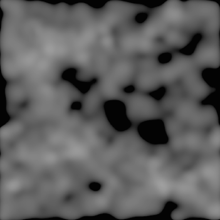
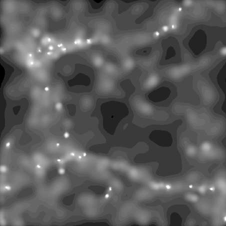
Figure 6: Evolution of a Gaussian density field with $P(k)\propto 1/k^{2}$: Initial condition (left side) and after one free-fall time (to the right). The density is normalised equally and scaled logarithmically in both images. The simulation was done with fully periodic GrapeSPH code using $100\,000$ particles.

Molecular clouds are highly structured: Observations reveal a hierarchy of filaments and sheets, clumps and sub-clumps, ranging from scales of the size of the whole cloud (see e.g. Bally 1996) down to the smallest objects resolved by todays telescopes (Wiseman & Ho 1996). Density-size or linewidth-size relations indicate that typically a cloud is to a large extent supported by “turbulent motion”; the measured linewidths exceed the thermal line broadening by far. Observations of Zeeman splitting and polarisation indicate the presence of magnetic fields. Furthermore feedback mechanisms from newly formed stars, outflows, stellar winds, ionization fronts and finally supernovae, produce shells and bubbles and deposit huge amounts of energy and momentum into the interstellar medium. The physical processes in molecular clouds are extremely diverse. A comprehensive overview can be found in “Protostars and Planets III”, eds. Levy & Lunine, 1993)

However, this is the environment in which stars form. To assess the problem of fragmentation and clump formation that leads to star formation, we start in the most basic way: We follow the dynamical evolution of isothermal gas in a region in the interior of a molecular cloud, starting from an initial density distribution to the formation of selfgravitating clumps. We solve the hydrodynamical equations using the SPH with Grape and implement periodic boundary conditions as described above to prevent global collapse. Ignoring additional physical effects, we study the interplay between gravity and gas pressure, which by itself will produce hierarchical filamentary structure, as was derived by de Vega, Sanchez & Combes (1996). Figure 6 describes one simulation: The left image is the projection of the initial density field, that was assumed to be Gaussian with a $1/k^{2}$ power spectrum. The right image depicts the same field after one free-fall time. The initial Gaussian fluctuations evolved into a system of filaments and knots, some of which contain collapsing cores. The initial conditions in Fig. 6 where chosen to be very cold; the total mass in the system exceeds the Jeans mass by far and a large number of initial density peaks are selfgravitating and begin to collapse. Gravity dominates strongly over pressure forces.

Figure 7 shows the mass distribution of the identified clumps. We divide the mass range into equal logarithmic intervals and plot the number of clumps identified, divided by the interval. For masses below $m\simeq 0.001$, our clump finding algorithm deteriorates and the sampling gets incomplete. With the chosen initial conditions and parameters, the mass distribution follows a power law, $dN/dm\propto m^{n}$, with $n\simeq-1.5$, which is indicated by the dashed line. This is in agreement with the values observed in molecular clouds (see e.g. Blitz 1993) although the observations exhibit a huge scatter. These results of our study of the fragmentation process in molecular clouds are still preliminary; more details will be discussed in a subsequent paper (Klessen & Burkert 1997).

Certainly this treatment is very coarse. It neglects the presence of magnetic fields and the input of energy and momentum by young stars. Future numerical studies of the evolution of interstellar medium and the formation of stars have to take these processes into account. However, the simple isothermal model presented here is able to reproduce some of the observed properties of giant molecular clouds and star forming regions.

Figure 7: Mass distribution of the identified clumps. The dashed line indicates the slope $dN/dm\propto m^{-1.5}$. The total mass in the system is $m=1$; for clump masses $m<0.001$ the sample gets incomplete.

6 Summary

We have presented a method of how to incorporate periodic boundary conditions into numerical simulations using the special hardware device Grape. We compute a periodic correction force onto each particle applying a particle-mesh like scheme: The particle forces in the isolated system are calculated via direct summation on the Grape board. Then we assign the particle distribution to a mesh and compute the periodic correction force for each grid point by convolution with the appropriate Green’s function in Fourier space. These forces are assigned back onto the individual particles. This method unites the advantages of Grape as being Lagrangian and offering good spacial resolution necessary for treating highly structured density distributions with the advantage of particle-mesh schemes as being intrinsically periodic. The potential of strong density peaks is dominated by the local mass accumulation. In such a region the influence of the global properties of the system is week and it is therefore sufficient to compute the correction term on relatively coarse grid. This keeps the additional computational cost low.

The method proposed here has proved to be numerically stable and inexpensive in terms of computer time. Thus the special purpose hardware device Grape can be applied successfully to astrophysical problems that require the correct treatment of periodic boundary conditions. As an example we study the dynamical evolution and fragmentation process in the interior of molecular clouds.

References

- [] Bally, J.: 1996, Nature, 382, 114
- [] Barnes, J.E., Hut, P.: 1986, Nature, 324, 446
- [] Bate, M.R., Bonnell, I.A., Price, N.M.: 1995, MNRAS, 277, 362
- [] Benz, W.: 1990, in The Numerical Modelling of Nonlinear Stellar Pulsations, p. 269-288, ed. J.R. Buchler, Kluwer Academic Publishers
- [] Blitz, L.: 1993, in Protostars and Planets III, p. 125, eds. E.H. Levy & J.I. Lunine, University of Arizona Press, Tucson & London
- [] Brieu, P.P., Summers, F.J., Ostriker, J.P.: 1995, ApJ, 453, 566
- [] Davé, R., Dubinski, J., Hernquist, L.: 1997, New Astronomy, submitted (astro-ph/9701113)
- [] de Vega, H.J., Sanchez, N., Combes, F.: 1996, Nature, 383, 139
- [] Ebisuzaki, T., Makino, J., Fukushige, T., Taiji, M., Sugimoto, D., Ito, T., Okumura, S.: 1993, PASJ, 45, 269
- [] Ewald, P.P.: 1921, Ann. Physik, 64, 253
- [] Fukushige, T., Makino, J., Ito, T., Okumura, S.K., Ebisuzaki, T., Sugimoto, D.: 1993, PASJ, 45, 361
- [] Fukushige, T., Taiji, M., Makino, J., Ebisuzaki, T., Sugimoto, D.: 1996, ApJ, 468, 51
- [] Hernquist, L., Katz, N.: 1989, ApJSS, 70, 419
- [] Hernquist, L., Bouchet, F.R., Suto, Y.: 1991, ApJSS, 75, 231
- [] Hockney, R.W., Eastwood, J.W.: 1988, Computer simulation using particles, IOP Publishing Ltd., Bristol and Philadelphia
- [] Huss, A., Jain, B., Steinmetz, M.: 1997, MNRAS, submitted
- [] Katz, N., Weinberg, D.H., Hernquist, L.: 1996, ApJSS, 105, 19
- [] Klessen, R., Burkert, A.: 1997, in preparation
- [] Levy, E.H., Lunine, J.I.: 1993, Protostars and Planets III, University of Arizona Press, Tucson & London
- [] Makino, J.,Fukushige, T., Okumura, S.K., Ebisuzaki, T.: 1993a, PASJ, 42, 303
- [] Makino, J., Funato, Y.: 1993, PASJ, 42, 279
- [] Makino, J., Hut, P.: 1997, PASP in press
- [] Makino, J., Ito, T., Ebisuzaki, T.: 1993, PASJ, 45, 329
- [] Makino, J., Kokubo, E., Taiji, M.: 1993, PASJ, 45, 349
- [] Monaghan, J.J.: 1992, ARA&A, 30, 543
- [] Okumura, S.K., Makino, J., Ebisuzaki, T., Fukushige, T., Ito, T., Sugimoto, D.: 1993, PASJ, 45, 329
- [] Press, W.H., Flannery, B.P., Teukolsky, S.A., Vetterling, W.T.: 1989, Numerical Recipies, Cambridge Univ. Press, Cambridge
- [] Steinmetz, M.: 1996, MNRAS, 278, 1005
- [] Sugimoto, D., Chikada, Y., Makino, J., Ito, T., Ebisuzaki, T., Umemura, M.: 1990, Nature, 345, 33
- [] Umemura, M., Fukushige, T., Makino, J., Ebisuzaki, T., Sugimoto, D., Turner, E.L., Loeb, A.: 1993, PASJ, 45,311
- [] Wiseman, J.J., Ho, P.T.P.: 1996, Nature, 382, 139