THE COSMOLOGY OF NOTHING

For more seventy years physicists have appreciated that Nature’s vacuum is far from empty. The discovery of the Lamb shift in Hydrogen provided dramatic verification of the reality of the quantum vacuum. The advent of gauge theories has led us to believe that the physics of the vacuum is even richer, with the possibility of instantons, vacuum phase transitions, vacuum defects (monopoles, domain walls, cosmic strings and nontopological solitons), vacuum energy, and degenerate vacua states (with different local realizations of the laws of physics). Cosmology offers a unique laboratory for exploring the “physics of nothing.” In this lecture I focus on the implications of vacuum energy for cosmology – in particular, inflation – and discuss the flood of observations that are testing the inflationary paradigm and in process probing the physics of nothing. I also discuss the possibility that today vacuum energy plays a dynamically important role (as a cosmological constant).

1 The Vacuum in Cosmology

The seminal papers of ’t Hooft$\!{}^{{\bf?}}$ and Polyakov$\!{}^{{\bf?}}$ revealed new richness in the physics of gauge theories – the existence of vacuum defects (topological solitons). Among the vacuum defects are magnetic monopoles, cosmic string, and domain walls.$\!{}^{{\bf?}}$ In addition, there are related objects such as textures $\!{}^{{\bf?}}$ and nontopological solitions.$\!{}^{{\bf?}}$ (The structure of the vacuum manifold determines the kind of defects that can arise in a theory.)

Unfortunately, it is unlikely that any of these interesting objects will ever be produced in terrestrial laboratories. However, the realization that spontaneously broken symmetries are restored at high temperature $\!{}^{{\bf?}}$ has made the early Universe a marvelous laboratory for studying vacuum defects, as they should be copiously produced in comological phase transitions associated with spontaneous symmetry breaking. The reason is simple: Owing to the existence of cosmological horizons, there is a maximum correlation distance (of order $ct$); on larger scales gauge and Higgs fields cannot be correlated which results in of order one defect per horizon volume.

Vacuum defects have a host of interesting cosmological consequences:$\!{}^{{\bf?}}$ seeding the formation of large-scale structure (global monopoles, cosmic strings and textures), producing a detectable background of gravitational waves and ultra high-energy cosmic rays (cosmic string), giving rise to the baryon asymmetry (cosmic string), gravitational lensing of distant objects (cosmic string), releasing large amounts of energy (superconducting cosmic string), and comprising the dark matter (nontopological solitons).

My focus in this lecture will be vacuum energy itself. During a phase transition the Universe can get “hung up” in a local minimum of the free energy. The associated “false-vacuum” energy can be dynamically important, driving a very rapid expansion, dubbed inflation by Guth in 1980.$\!{}^{{\bf?}}$ (In fact, rapid expansion driven by the potential energy of a scalar field is much more general than phase transitions.)

As I will describe in this lecture, inflation has profound consequences for cosmology, possibly providing answers to the most pressing and fundamental questions. I will also discuss the possibility that vacuum energy is playing an important dynamical role in the Universe today. Here vacuum and cosmology come full circle: Einstein originally suggested the possibility of a cosmological constant (which is mathematically equivalent to a vacuum energy density) to obtain static cosmological solutions. He later discarded it when Hubble discovered the expansion of the Universe. Once again the observations suggest the need for a cosmological constant.

Inflation has probably been the single most influential idea in cosmology during the past decade. So much so that it has set the observational agenda. And now the observations are beginning to sharply test inflation and with it the physics of the vacuum. To set the stage, let me begin with the a brief discussion of the standard cosmology.

2 Standard Cosmology

2.1 Status

The Hot Big-bang Cosmology is a remarkable achievement. It provides a reliable account of the Universe from about $10^{-2}\,{\rm sec}$ to the present.$\!{}^{{\bf?}}$ Further, the hot big-bang model together with modern ideas in particle physics—the Standard Model, supersymmetry, grand unification, and superstring theory— provide a sound framework for sensible speculation all the way back to the Planck epoch and perhaps even earlier.

These speculations have allowed cosmologists to address a deeper set of questions: What is the nature of the ubiquitous dark matter that is the dominant component of the mass density? Why does the Universe contain only matter? What is the origin of the tiny inhomogeneities that seeded the formation of structure, and how did that structure evolve? Why is the portion of the Universe that we can see so flat and smooth? What is the value of the cosmological constant? How did the expansion begin—or was there a beginning? What was the big bang?

In the past fifteen years much progress has been made, and many believe that the answers to all these questions involve events that took place during the earliest moments and involved physics beyond the Standard Model.$\!{}^{{\bf?}}$ For example, the matter-antimatter asymmetry, quantified as a net baryon number of about $10^{-10}$ per photon, is believed to have developed through interactions that do not conserve baryon number or $C$, $CP$ and occurred out of thermal equilibrium. If “baryogenesis” involved unification-scale physics the baryon asymmetry developed around $10^{-34}\,{\rm sec}$; on the other hand, baryogenesis might have occurred at the weak scale ($T\sim 300\,{\rm GeV}$ and $t\sim 10^{-11}\,{\rm sec}$) through baryon-number violation within the Standard Model and $C$, $CP$ violation from physics beyond the Standard Model.$\!{}^{{\bf?}}$

The most optimistic early-Universe cosmologists (of which I am one) believe that we are on the verge of solving all of the above problems and extending our knowledge of the Universe back to around $10^{-32}\,{\rm sec}$ after “the bang.” The key is inflation. Among other things, inflation has led to the cold dark matter model of structure formation, whose basic tenets are scale-invariant density perturbations and dark matter whose primary composition is slowly moving elementary particles (e.g., axions or neutralinos). Cold dark matter provides a crucial test of inflation and a possible window to physics at unification-scale energies. If cold dark matter is correct, it would complete the standard cosmology by connecting the theorist’s smooth early Universe to the astronomer’s Universe which abounds with structure, galaxies, clusters of galaxies, superclusters, voids and great walls.$\!{}^{{\bf?}}$ Thanks to a flood of data, cold dark matter and inflation are being tested more and more sharply.

2.2 Evidence

Four pillars provide the observational support on which the hot big-bang model rests: (1) The uniform distribution of matter on large scales and the isotropic expansion that maintains this uniformity; (2) The existence of a nearly uniform and accurately thermal cosmic background radiation (CBR); (3) The abundances (relative to hydrogen) of the light elements D, ³He, ⁴He, and ⁷Li (see Fig. 1); and (4) The existence of small fluctuations in the temperature of the CBR across the sky, at the level about $10^{-5}$ (see Fig. 2). The validity of Hubble’s expansion law, $z\simeq H_{0}d$, out to redshifts $z\sim 0.2$ supports the general notion of an expanding Universe, and the CBR provides almost indisputable evidence of a hot, dense beginning. The agreement between the light-element abundances predicted by primordial nucleosynthesis and those observed in the most primitive samples of the cosmos tests the model back to about $10^{-2}\,{\rm sec}$ and leads to the most accurate determination of the baryon density.$\!{}^{{\bf?}}$ The small fluctuations in the temperature of CBR indicate the existence of primeval density perturbations of a similar size, which, amplified by gravity over the age of the Universe, seeded the abundance of structure seen today.

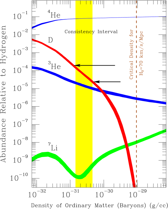
Figure 1: Summary of big-bang production of the light elements. The widths of the curves indicate the $2\sigma$ theoretical uncertainties, and the vertical band is the consistency interval where the abundances of all four light elements agree with their measured primeval abundances. The critical density, which depends upon the square of the Hubble constant, is indicated for $H_{0}=70\,{\rm km\,s^{-1}}\,{\rm Mpc}^{-1}$. The two arrows indicate the largest and smallest deuterium abundances reported in high redshift hydrogen clouds (see Refs. 9). Figure courtesy of C. Copi.

Figure 2: Summary of CBR anisotropy measurements and predictions for three CDM models (adapted from Ref. 13). Plotted are the squares of the measured multipole amplitudes ($C_{l}=\langle|a_{lm}|^{2}\rangle$) in units of $7\times 10^{-10}$ vs. multipole number $l$ The temperature difference on angular scale $\theta$ is given roughly by $\sqrt{l(l+1)C_{l}}$ with $l\sim 200^{\circ}/\theta$. The theoretical curves are standard CDM and CDM with $n=0.7$ and $h=0.5$.

2.3 New Results

The flood of data in cosmology is not only testing inflation and cold dark matter, it is also establishing fundamental aspects of the standard cosmology itself. I mention four new results.

According to the big-bang model the temperature of the CBR decreases as the Universe expands, and a recent measurement has confirmed this prediction.$\!{}^{{\bf?}}$ The relative populations of hyperfine states in neutral Carbon atoms seen in a gas cloud at redshift $z=1.776$ indicate a thermodynamic temperature, $7.4\pm 0.8\,$K, which is consistent with the big-bang prediction for the CBR temperature at this earlier time, $T(z)=(1+z)2.728\,{\rm K}=7.58\,$K.

While many cite the discovery of CBR anisotropy as COBE’s most important result, its measurement of the spectrum of the CBR is at least as impressive. The Far Infrared Absolute Spectrometer (FIRAS) on COBE: (1) established that the spectrum of the CBR is a perfect black-body with deviations that are less than 0.03% of the peak intensity (95% CL upper limits to the distortion parameters: $|\mu|<9\times 10^{-5}$ and $y<15\times 10^{-6}$); (ii) determined the CBR temperature to four significant figures, $T=2.728\,{\rm K}\pm 0.002\,{\rm K}$; (iii) measured the amplitude ($3.372\,{\rm mK}\pm 0.0035\,{\rm mK}$), direction (galactic coordinates $l,b=264.14^{\circ}\pm 0.15^{\circ},48.26^{\circ}\pm 0.15^{\circ}$) and spectrum (consistent with black-body temperature $2.717\,{\rm K}\pm 0.007\,{\rm K}$) of the dipole anisotropy.$\!{}^{{\bf?}}$

The big-bang abundance of deuterium, with its rapid variation with the baryon density, has long been recognized as the ultimate “baryometer.” That dream is becoming reality thanks to the Keck 10 meter Telescope. There have now been seven detections of deuterium in high redshift ($z\sim 2-4$), metal-poor hydrogen clouds (seen in absorption in the spectra of high redshift QSOs).$\!{}^{{\bf?}}$ The measured deuterium abundance (relative to H) ranges from $2\times 10^{-5}$ to $2\times 10^{-4}$, as anticipated from the abundances of the other light elements, though the scatter in the measured values is larger than the estimated errors. A measurement of the deuterium abundance to 15% – which seems likely within a few years – would pin down the baryon density to 10%, provide an important confirmation of big-bang nucleosynthesis, and sharpen nucleosynthesis as a probe of particle physics.

The Hubble constant may be finally coming into focus. The detection of individual Cepheid variable stars in Virgo-cluster galaxies by the Hubble Space Telescope and the calibration of Type Ia supernovae as standard candles represent major milestones in the quest for $H_{0}$.$\!{}^{{\bf?}}$ The range favored by current observations is $60\,{\rm km\,s^{-1}}\,{\rm Mpc}^{-1}$ to $80\,{\rm km\,s^{-1}}\,{\rm Mpc}^{-1}$, which is “in tension” with measurements of the age of the oldest stars, between $13\,{\rm Gyr}$ and $19\,{\rm Gyr}$ (see Fig. 3).$\!{}^{{\bf?}}$ I will return to this point later.

Figure 3: Isochrones in the $H_{0}$ - $\Omega_{\rm Matter}$ plane. The bottom band corresponds to time back to the bang of between $13\,{\rm Gyr}$ and $19\,{\rm Gyr}$; the lightest band to between $10\,{\rm Gyr}$ and $13\,{\rm Gyr}$; the darkest region is disallowed: $\Omega_{\rm Matter}<0.3$ or expansion time less than $10\,{\rm Gyr}$. Broken horizon lines indicate the range favored for the Hubble constant, $80\,{\rm km\,s^{-1}}\,{\rm Mpc}^{-1}>H_{0}>60\,{\rm km\,s^{-1}}\,{\rm Mpc}^{-1}$. The age – Hubble constant tension is clear, especially for the inflationary prediction of $\Omega_{\rm Matter}=1$. The broken curves denote the $13\,{\rm Gyr}-19\,{\rm Gyr}$ isochrone for $\Lambda$CDM; a cosmological constant greatly lessens the tension.

3 Inflation

As successful as the big-bang cosmology is, it suffers from a dilemma involving initial data. Extrapolating back, one finds that the Universe apparently began from a very special state: A slightly inhomogeneous and very flat Robertson-Walker spacetime. Collins and Hawking showed that the set of initial data that evolve to a spacetime that is as smooth and flat as ours is today of measure zero.$\!{}^{{\bf?}}$ (In the context of simple grand unified theories, the hot big-bang model suffers from another serious problem: the extreme overproduction of superheavy magnetic monopoles; in fact, attempting to solve the monopole problem led Guth to inflation.)

The cosmological appeal of inflation is the lessening of the dependence of the present state of the Universe upon the initial state. Two elements are essential: (1) accelerated (“superluminal”) expansion and the concomitant tremendous growth of the scale factor; and (2) massive entropy production.$\!{}^{{\bf?}}$ Through inflation, a small, smooth subhorizon-sized patch of the early Universe grows to a large enough size and comes to contain enough heat (entropy in excess of $10^{88}$) to encompass our present Hubble volume. In addition, superluminal expansion guarantees that the Universe today appears flat (just as any small portion of the surface of a large sphere appears flat).

While there is presently no standard model of inflation—just as there is no standard model for physics at these energies (typically $10^{15}\,{\rm GeV}$ or so)—viable models have much in common. They are based upon well posed, albeit highly speculative, microphysics involving the classical evolution of a scalar field. A nearly exponential expansion is driven by the potential energy (“vacuum energy”) that arises when the scalar field is displaced from its potential-energy minimum. Provided the potential is flat, during the time it takes for the field to roll to the minimum of its potential the Universe undergoes many e-foldings of expansion (more than around 60 or so are required to realize the beneficial features of inflation). As the scalar field nears the minimum, the vacuum energy has been converted to coherent oscillations of the scalar field, which correspond to nonrelativistic scalar-field particles. The eventual decay of these particles into lighter particles and their thermalization results in the “reheating” of the Universe and accounts for all the heat in the Universe today (the entropy production event).

The tremendous growth of the cosmic scale factor (by a factor greater than that since the end of inflation) allows quantum fluctuations excited on very small scales ($\mathrel{\mathchoice{\lower 3.6pt\vbox{\halign{$\mathsurround=0pt\displaystyle\hfil#\hfil$\cr<\crcr\sim\crcr}}}{\lower 3.6pt\vbox{\halign{$\mathsurround=0pt\textstyle\hfil#\hfil$\cr<\crcr\sim\crcr}}}{\lower 3.6pt\vbox{\halign{$\mathsurround=0pt\scriptstyle\hfil#\hfil$\cr<\crcr\sim\crcr}}}{\lower 3.6pt\vbox{\halign{$\mathsurround=0pt\scriptscriptstyle\hfil#\hfil$\cr<\crcr\sim\crcr}}}}10^{-23}\,{\rm cm}$) to be stretched to astrophysical scales ($\mathrel{\mathchoice{\lower 3.6pt\vbox{\halign{$\mathsurround=0pt\displaystyle\hfil#\hfil$\cr>\crcr\sim\crcr}}}{\lower 3.6pt\vbox{\halign{$\mathsurround=0pt\textstyle\hfil#\hfil$\cr>\crcr\sim\crcr}}}{\lower 3.6pt\vbox{\halign{$\mathsurround=0pt\scriptstyle\hfil#\hfil$\cr>\crcr\sim\crcr}}}{\lower 3.6pt\vbox{\halign{$\mathsurround=0pt\scriptscriptstyle\hfil#\hfil$\cr>\crcr\sim\crcr}}}}10^{25}\,{\rm cm}$). Quantum fluctuations in the scalar field responsible for inflation ultimately lead to an almost scale-invariant spectrum of density perturbations,$\!{}^{{\bf?}}$ and quantum fluctuations in the metric itself lead to an almost scale-invariant spectrum of gravity-waves.$\!{}^{{\bf?}}$ Scale invariance for density perturbations means scale-independent fluctuations in the gravitational potential (equivalently, density perturbations of different wavelength cross the horizon with the same amplitude); scale invariance for gravity waves means that gravity waves of all wavelengths cross the horizon with the same amplitude. Because of subsequent evolution, neither the scalar nor the tensor perturbations are scale invariant today.

3.1 Grander Implications

Inflation alleviates the “specialness” problem greatly, but does not eliminate it.$\!{}^{{\bf?}}$ All open FRW models will inflate and become flat; however, many closed FRW models will recollapse before they can inflate. If one imagines the most general initial spacetime as being comprised of negatively and positively curved FRW (or Bianchi) models that are stitched together, the failure of the positively curved regions to inflate is of little consequence: because of exponential expansion during inflation the negatively curved regions will occupy most of the space today. Inflation does not solve the smoothness problem forever; it just postpones the problem into the exponentially distant future: We will be able to see outside our smooth inflationary patch and $\Omega$ will start to deviate significantly from unity at a time $t\sim t_{0}\exp[3(N-N_{\rm min}]$, where $N$ is the actual number of e-foldings of inflation and $N_{\rm min}\sim 60$ is the minimum required to solve the horizon/flatness problems.

Linde has emphasized that inflation has changed our view of the Universe in a very fundamental way.$\!{}^{{\bf?}}$ While cosmologists have long used the Copernician principle to argue that the Universe must be smooth because of the smoothness of our Hubble volume, in the post-inflation view, our Hubble volume is smooth because it is a small part of a region that underwent inflation. On the largest scales the structure of the Universe is likely to be very rich: Different regions may have undergone different amounts of inflation, may have different realizations of the laws of physics because they evolved into different vacuum states (of equivalent energy), and may even have different numbers of spatial dimensions. Since it is likely that most of the volume of the Universe is still undergoing inflation and that inflationary patches are being constantly produced (eternal inflation), the age of the Universe is a meaningless concept and our expansion age merely measures the time back to our big bang – the nucleation of our inflationary bubble.

3.2 Specifics

Guth’s seminal paper$\!{}^{{\bf?}}$ both introduced the idea of inflation and showed that the model that he based the idea upon did not work! Thanks to very important contributions by Linde$\!{}^{{\bf?}}$ and Albrecht and Steinhardt$\!{}^{{\bf?}}$ that was quickly remedied, and today there are many viable models of inflation. That of course is good news and bad news – since it means that there is no standard model of inflation. The absence of a standard model of inflation should of course be viewed in the light of our general ignorance about physics at unification-scale energies.

Many different approaches have taken in constructing particle-physics models for inflation. Some have focussed on very simple scalar potentials, e.g., $V(\phi)=\lambda\phi^{4}$ or $=m^{2}\phi^{2}/2$, without regard to connecting the model to any underlying theory.$\!{}^{{\bf?},{\bf?}}$ Others have proposed more complicated models that attempt to make contact with speculations about physics at very high energies, e.g., grand unification,$\!{}^{{\bf?}}$ supersymmetry,$\!{}^{{\bf?},{\bf?},{\bf?},{\bf?}}$ preonic physics,$\!{}^{{\bf?}}$ or supergravity.$\!{}^{{\bf?}}$ Several authors have attempted to link inflation with superstring theory$\!{}^{{\bf?}}$ or “generic predictions” of superstring theory such as pseudo-Nambu-Goldstone boson fields.$\!{}^{{\bf?}}$ While the scale of the vacuum energy that drives inflation is typically of order $(10^{15}\,{\rm GeV})^{4}$, a model of inflation at the electroweak scale, vacuum energy $\approx(1\,{\rm TeV})^{4}$, has been proposed.$\!{}^{{\bf?}}$ There are also models in which there are multiple epochs of inflation.$\!{}^{{\bf?}}$

In all of the models above gravity is described by general relativity. A qualitatively different approach is to consider inflation in the context of alternative theories of gravity. (After all, inflation probably involves physics at energy scales not too different from the Planck scale and the effective theory of gravity at these energies could well be very different from general relativity; in fact, there are some indications from superstring theory that gravity in these circumstances might be described by a Brans-Dicke like theory.) The most successful of these models is first-order inflation.$\!{}^{{\bf?},{\bf?}}$ First-order inflation returns to Guth’s original idea of a strongly first-order phase transition; in the context of general relativity Guth’s model failed because the phase transition, if inflationary, never completed. In theories where the effective strength of gravity evolves, like Brans-Dicke theory, the weakening of gravity during inflation allows the transition to complete. In other models based upon nonstandard gravitation theory, the scalar field responsible for inflation is itself related to the size of additional spatial dimensions, and inflation then also explains why our three spatial dimensions are so big, while the other spatial dimensions are so small.

All models of inflation have one feature in common: the scalar field responsible for inflation has a very flat potential-energy curve and is very weakly coupled. Invariably, this leads to a very small dimensionless number, usually a coupling constant of the order of $10^{-14}$. Such a small number, like other small numbers in physics (e.g., the ratio of the weak to Planck scales $\approx 10^{-17}$ or the ratio of the mass of the electron to the $W/Z$ boson masses $\approx 10^{-5}$), runs counter to one’s belief that a truly fundamental theory should have no tiny parameters, and cries out for an explanation. At the very least, this small number must be stabilized against quantum corrections—which it is in all of the previously mentioned models. In some models, the small number in the inflationary potential is related to other small numbers in particle physics: for example, the ratio of the electron mass to the weak scale or the ratio of the unification scale to the Planck scale. Explaining the origin of the small number that seems to be associated with inflation is both a challenge and an opportunity.

Because of the growing base of observations that bear on inflation, another approach to model building is emerging: the use of observations to constrain the underlying inflationary model. In Section 4 I will discuss the possibilities for reconstructing the inflationary potential.

3.3 Three Robust Predictions

While there are many varieties of inflation, there are three robust predictions which are crucial to sharply testing inflation.

1. Flat universe. Because solving the “horizon” problem (large-scale smoothness in spite of small particle horizons at early times) and solving the “flatness” problem (maintaining $\Omega$ very close to unity until the present epoch) are linked geometrically,$\!{}^{{\bf?},{\bf?}}$ this is the most robust prediction of inflation. Said another way, it is the prediction that most inflationists would be least willing to give up. (Even so, models of inflation have been constructed where the amount of inflation is tuned just to give $\Omega_{0}$ less than one today.$\!{}^{{\bf?}}$) Through the Friedmann equation for the scale factor, flat implies that the total energy density (matter, radiation, vacuum energy, and anything else) is equal to the critical density.

2. Nearly scale-invariant spectrum of gaussian density perturbations. Essentially all inflation models predict a nearly scale-invariant spectrum of gaussian density perturbations. Described in terms of a power spectrum, $P(k)\equiv\langle|\delta_{k}|^{2}\rangle=Ak^{n}$, where $\delta_{k}$ is the Fourier transform of the primeval density perturbations, and the spectral index $n=1$ in the scale-invariant limit. The overall amplitude $A$ is model dependent. Density perturbations give rise to CBR anisotropy as well as seeding structure formation. Requiring that the density perturbations are consistent with the observed level of anisotropy of the CBR (and large enough to produce the observed structure formation) is the most severe constraint on inflationary models and leads to the small dimensionless number that all inflationary models have.

3. Nearly scale-invariant spectrum of gravitational waves. These gravitational waves have wavelengths from around $1\,{\rm km}$ to the size of the present Hubble radius and beyond. Described in terms of a power spectrum for the dimensionless gravity-wave amplitude at early times, $P_{T}(k)\equiv\langle|h_{k}|^{2}\rangle=A_{T}k^{n_{T}-3}$, where the spectral index $n_{T}=0$ in the scale-invariant limit. Once again, the overall amplitude $A_{T}$ is model dependent (varying as the value of the inflationary vacuum energy). Unlike density perturbations, which are required to initiate structure formation, there is no cosmological lower bound to the amplitude of the gravity-wave perturbations. Tensor perturbations also give rise to CBR anisotropy; requiring that they do not lead to excessive anisotropy implies that the energy density that drove inflation must be less than about $(10^{16}\,{\rm GeV})^{4}$. This indicates that if inflation took place, it did so at an energy well below the Planck scale.

There are other interesting consequences of inflation that are less generic. For example, in first-order inflation, where reheating occurs through the nucleation and collision of vacuum bubbles, there is an additional, larger amplitude, but narrow-band, spectrum of gravitational waves ($\Omega_{\rm GW}h^{2}\sim 10^{-6}$).$\!{}^{{\bf?}}$ In other models large-scale primeval magnetic fields of interesting size are seeded during inflation.$\!{}^{{\bf?}}$

I want to emphasize the importance of the tensor perturbations. The attractiveness of a flat Universe with scale-invariant density perturbations was appreciated long before inflation. Verifying these two predictions of inflation, while important, will not provide a “smoking gun.” A spectrum of nearly scale-invariant tensor perturbations is a defining feature of inflation, and further, is crucial to obtaining information about the underlying scalar potential.

CBR anisotropy probably provides the best possibility of detecting the tensor perturbations, but their contribution to CBR anisotropy has to be separated that of the scalar perturbations. Because the sky is finite, sampling variance sets a fundamental limit: the tensor contribution to CBR anisotropy can only be separated from that of the scalar if $T/S$ is greater than about $0.14$$\!{}^{{\bf?}}$ ($T$ is the contribution of tensor perturbations to the variance of the CBR quadrupole and $S$ is the same for scalar perturbations).

It is possible that the stochastic background of gravitational waves itself can be directly detected, though it appears that the LIGO facilities being built will lack the sensitivity and even space-based interferometery (e.g., LISA) is not a sure bet.$\!{}^{{\bf?}}$

4 Cold Dark Matter

Cold dark matter actually draws from three important ideas – inflation, big-bang nucleosynthesis, and the quest to better understand the fundamental forces and particles. As discussed above, inflation predicts a flat Universe (total energy density equal to the critical density) and nearly scale-invariant density perturbations. Big-bang nucleosynthesis provides the most precise determination of the density of ordinary matter, present density between $1.7\times 10^{-31}{\,{\rm g\,cm^{-3}}}$ and $4.1\times 10^{-31}{\,{\rm g\,cm^{-3}}}$, or fraction of critical density $\Omega_{B}=0.01h^{-2}-0.02h^{-2}$, where $H_{0}=100h\,{\rm km\,s^{-1}}\,{\rm Mpc}^{-1}$.$\!{}^{{\bf?}}$ Allowing $h=0.4-0.9$, consistent with modern measurements,$\!{}^{{\bf?}}$ implies that ordinary matter can contribute at most 15% of the critical density. If the inflationary prediction is correct, then most of the matter in the Universe must be nonbaryonic (see Fig. 4).

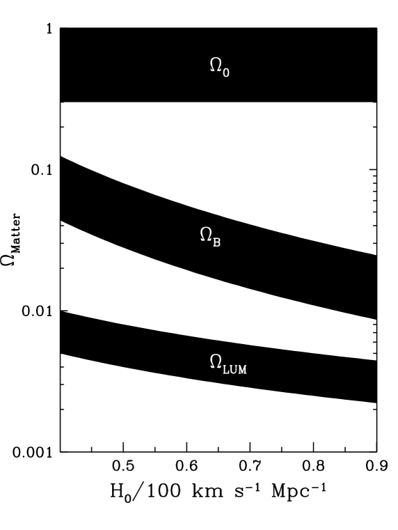
Figure 4: Summary of knowledge of $\Omega$. The lowest band is luminous matter, in the form of bright stars and related material; the middle band is the big-bang nucleosynthesis determination of the density of baryons; the upper region is the estimate of $\Omega_{\rm Matter}$ based upon the peculiar velocities of galaxies. The gaps between the bands illustrate the two dark matter problems: most of the ordinary matter is dark and most of the matter is nonbaryonic.

This idea has received indirect support from particle physics. Attempts to further our understanding of the particles and forces have led to the prediction of new, stable or long-lived particles that interact very feebly with ordinary matter. These particles, if they exist, should have been present in great numbers during the earliest moments and remain today in numbers sufficient to contribute the critical density.$\!{}^{{\bf?}}$ Two of the most attractive possibilities behave like cold dark matter: a neutralino of mass $10\,{\rm GeV}$ to $1000\,{\rm GeV}$, predicted in supersymmetric theories, and an axion of mass $10^{-6}{\,\rm eV}$ to $10^{-4}{\,\rm eV}$, needed to solve a subtle problem of the standard model of particle physics (strong-CP problem). The third interesting possibility is that one of the three neutrino species has a mass between $5{\,\rm eV}$ and $30{\,\rm eV}$; neutrinos move very fast and are referred to as hot dark matter.

According to cold dark matter theory CDM particles provide the cosmic infrastructure: It is their gravitational attraction that forms and holds cosmic structures together. Structure forms in a hierarchical manner, with galaxies forming first and successively larger objects forming thereafter.$\!{}^{{\bf?}}$ Quasars and other rare objects form at redshifts of up to five, with ordinary galaxies forming a short time later. Today, superclusters, objects made of several clusters of galaxies, are just becoming bound by the gravity of their CDM constituents. The formation of larger and larger objects continues. In the clustering process regions of space are left devoid of matter – and galaxies – leading to voids.

If the CDM theory is correct, CDM particles are the ubiquitous dark matter known only by its gravitational effects which accounts for most of the mass density in the Universe and holds galaxies, clusters of galaxies and even the Universe itself together.$\!{}^{{\bf?}}$

4.1 Standard Cold Dark Matter

When the cold dark matter scenario emerged more than a decade ago many referred to it as a no parameter theory because it was so specific compared to previous models for the formation of structure. This was an overstatement as there are cosmological quantities that must be known to determine the development of structure in detail. However, the data available did not require precise knowledge of these quantities to test the model.

Broadly speaking these parameters can be organized into two groups. First are the cosmological parameters: the Hubble constant, specified by $h$; the density of ordinary matter, specified by $\Omega_{B}h^{2}$; the power-law index $n$ and normalization $A$ that quantify the density perturbations; and the amplitude and spectral index $n_{T}$ that quantify the gravitational waves. The inflationary parameters fall into this category because there is no standard model of inflation. On the other hand, once determined they can be used to discriminate between models of inflation.

The other quantities specify the composition of invisible matter in the Universe: radiation, dark matter, and a possible cosmological constant. Radiation refers to relativistic particles: the photons in the CBR, three massless neutrino species (assuming none of the neutrino species has a mass), and possibly other undetected relativistic particles (some particle-physics theories predict the existence of additional massless particle species). At present relativistic particles contribute almost nothing to the energy density in the Universe, $\Omega_{R}\simeq 4.2\times 10^{-5}h^{-2}$; early on – when the Universe was smaller than about $10^{-5}$ of its present size – they dominated the energy content.

In addition to CDM particles, the dark matter could include other particle relics. For example, each neutrino species has a number density of $113{\,{\rm cm}^{-3}}$, and a neutrino species of mass $5{\,\rm eV}$ would account for about 20% of the critical density ($\Omega_{\nu}=m_{\nu}/90h^{2}{\,\rm eV}$). Predictions for neutrino masses range from $10^{-12}{\,\rm eV}$ to several MeV, and there is some experimental evidence that at least one of the neutrino species has a small mass.$\!{}^{{\bf?}}$

Finally, there is the cosmological constant. Both introduced and abandoned by Einstein, it is still with us. In the modern context it corresponds to an energy density associated with the quantum vacuum. At present, there is no reliable calculation of the value that the cosmological constant should take, and so its existence must be regarded as a logical possibility.

The original no parameter cold dark matter model, referred to as standard CDM, is characterized by: $h=0.5$, $\Omega_{B}=0.05$, $\Omega_{\rm CDM}=0.95$, $n=1$, no gravitational waves and standard radiation content. The overall normalization of the density perturbations was fixed by comparing the predicted level of inhomogeneity with that seen today in the distribution of bright galaxies. Specifically, the amplitude $A$ was determined by comparing the expected mass fluctuations in spheres of radius $8h^{-1}\,{\rm Mpc}$ (denoted by $\sigma_{8}$) to the galaxy-number fluctuations in spheres of the same size. The galaxy-number fluctuations on the scale $8h^{-1}\,{\rm Mpc}$ are unity; adjusting $A$ to achieve $\sigma_{8}=1$ corresponds to the assumption that light, in the form of bright galaxies, traces mass. Choosing $\sigma_{8}$ to be less than one means that light is more clustered than mass and is a biased tracer of mass. There is some evidence that bright galaxies are somewhat more clumped than mass with biasing factor $b\equiv 1/\sigma_{8}\simeq 1-2$.$\!{}^{{\bf?}}$

A dramatic change occurred with the detection of CBR anisotropy by COBE in 1992.$\!{}^{{\bf?}}$ The COBE measurement permitted a precise normalization of the amplitude of density perturbations on very large scales ($\lambda\sim 10^{4}h^{-1}\,{\rm Mpc}$) without regard to the issue of biasing. [CBR anisotropy on the angular scale $\theta$ arises primarily due to inhomogeneity on length scales $\lambda\sim 100h^{-1}\,{\rm Mpc}(\theta/{\rm deg})$.] For standard CDM, the COBE normalization leads to: $\sigma_{8}=1.2\pm 0.1$ or anti-bias since $b=1/\sigma_{8}\simeq 0.7$. The pre-COBE normalization ($\sigma_{8}=0.5$) led to too little power on scales of $30h^{-1}\,{\rm Mpc}$ to $300h^{-1}\,{\rm Mpc}$, as compared to what was indicated in redshift surveys, the angular correlations of galaxies on the sky and the peculiar velocities of galaxies. The COBE normalization leads to about the right amount of power on these scales, but appears to predict too much power on small scales ($\mathrel{\mathchoice{\lower 3.6pt\vbox{\halign{$\mathsurround=0pt\displaystyle\hfil#\hfil$\cr<\crcr\sim\crcr}}}{\lower 3.6pt\vbox{\halign{$\mathsurround=0pt\textstyle\hfil#\hfil$\cr<\crcr\sim\crcr}}}{\lower 3.6pt\vbox{\halign{$\mathsurround=0pt\scriptstyle\hfil#\hfil$\cr<\crcr\sim\crcr}}}{\lower 3.6pt\vbox{\halign{$\mathsurround=0pt\scriptscriptstyle\hfil#\hfil$\cr<\crcr\sim\crcr}}}}8h^{-1}\,{\rm Mpc}$); see Fig. 5.

While standard CDM is in general agreement with the observations, a consensus has developed that the conflict just mentioned is probably significant.$\!{}^{{\bf?}}$ This has led to a new look at the cosmological and invisible-matter parameters and to the realization that the problems of standard CDM are simply a poor choice for the standard parameters.

Figure 5: Measurements of the power spectrum, $P(k)=|\delta_{k}|^{2}$, and the predictions of different COBE-normalized CDM models. The points are from several redshift surveys as analyzed in Ref. 56; the models are: $\Lambda$CDM with $\Omega_{\Lambda}=0.6$ and $h=0.65$; standard CDM (sCDM), CDM with $h=0.35$; $\tau$CDM (with the energy equivalent of 12 massless neutrino species) and $\nu$CDM with $\Omega_{\nu}=0.2$ (unspecified parameters have their standard CDM values).

5 Flood of Data

5.1 Viable Models

Standard CDM has served well as an industry-wide standard that focused everyone’s attention – the DOS of cosmology. However, the quality and quantity of data have improved and knowledge of the cosmological and invisible-matter parameters has become important for serious testing of CDM and inflation. There are a variety of combinations of the parameters that lead to good agreement with the existing data on both large and small length scales – and thus can make a claim to being the new standard CDM model. Figure 6 shows the allowed values of the cosmological for several COBE-normalized CDM models.

More precisely, for a given CDM model – specified by the cosmological and invisible-matter parameters – the expected CBR anisotropy is computed and required to be consistent with the four-year COBE data set at the two-sigma level.$\!{}^{{\bf?}}$ The expected level of inhomogeneity in the Universe today and compare to three robust measurements of inhomogeneity: the shape of the power spectrum as inferred from surveys of the distribution of galaxies today;$\!{}^{{\bf?}}$ a determination of $\sigma_{8}$ based upon the abundance of rich, x-ray emitting clusters;$\!{}^{{\bf?}}$ and the abundance of hydrogen clouds at high redshift (which probes early structure formation).$\!{}^{{\bf?}}$

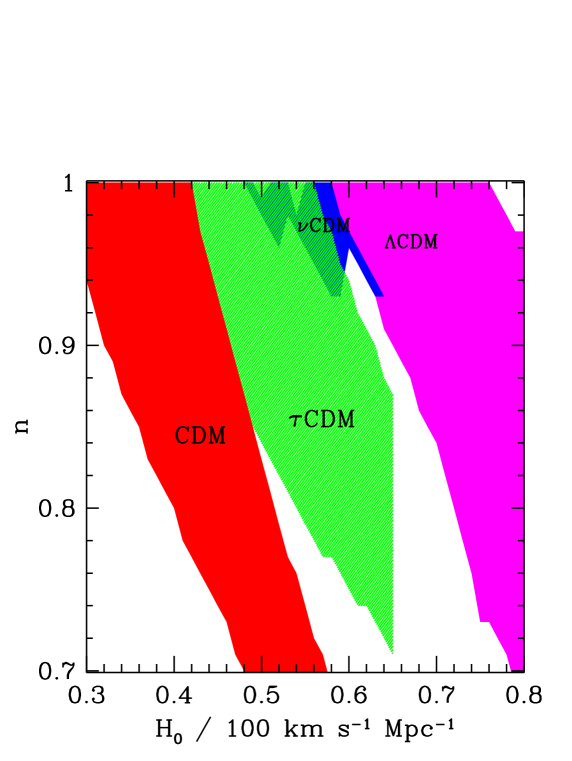
Figure 6: Acceptable values of the cosmological parameters $n$ and $h$ for CDM models with standard invisible-matter content (CDM), with 20% hot dark matter ($\nu$CDM), with additional relativistic particles (the energy equivalent of 12 massless neutrino species, denoted $\tau$CDM), and with a cosmological constant that accounts for 60% of the critical density ($\Lambda$CDM). Note that standard CDM ($n=1$ and $h=0.5$) is not viable.

Figure 6 summarizes the overall picture. The simplest CDM models – those with standard invisible-matter content – lie in a region that runs diagonally from smaller Hubble constant and larger $n$ to larger Hubble constant and smaller $n$. That is, higher values of the Hubble constant require more tilt (tilt referring to deviation from scale invariance). Note too that standard CDM is well outside of the allowed range. Current measurements of CBR anisotropy on the degree scale, as well as the COBE four-year anisotropy data, preclude $n$ less than about 0.7 (see Fig. 2). This implies that the largest Hubble constant consistent with the simplest CDM models is slightly less than $60\,{\rm km\,s^{-1}}\,{\rm Mpc}^{-1}$. If the invisible-matter content is nonstandard, higher values of the Hubble constant can be accommodated. In Fig. 6, $\Omega_{\nu}$ is taken to be 0.2; in fact, this is essentially the largest value allowed by measurements of the power spectrum.$\!{}^{{\bf?},{\bf?}}$ On the other hand, even $\Omega_{\nu}=0.05$ (around $1{\,\rm eV}$ worth of neutrinos) can have important consequences (e.g., accommodating a higher value of the Hubble constant or more nearly scale-invariant density perturbations).

Changes in the different parameters from their standard CDM values alleviate the excess power on small scales in different ways. Tilt has the effect of reducing power on small scales when power on very large scales is fixed by COBE. A small admixture of hot dark matter works because fast moving neutrinos suppress the growth of inhomogeneity on small scales by streaming from regions of higher density and to regions of lower density. (It was in fact this feature of hot dark matter that led to the demise of the hot dark matter model for structure formation.)

A low value of the Hubble constant, additional radiation or a cosmological constant all reduce power on small scales by lowering the ratio of matter to radiation. Since the critical density depends upon the square of the Hubble constant, $\rho_{\rm Critical}=3H_{0}^{2}/8\pi G$, a smaller value corresponds to a lower matter density since $\rho_{\rm Matter}=\rho_{\rm Critical}$ for a flat Universe without a cosmological constant. Shifting some of the critical density to vacuum energy also reduces the matter density since $\Omega_{\rm Matter}=1-\Omega_{\Lambda}$. Lowering the ratio of matter to radiation reduces the power on small scales in a subtle way. While the primeval fluctuations in the gravitational potential are nearly scale-invariant, density perturbations today are not because the Universe made a transition from an early radiation-dominated phase ($t\mathrel{\mathchoice{\lower 3.6pt\vbox{\halign{$\mathsurround=0pt\displaystyle\hfil#\hfil$\cr<\crcr\sim\crcr}}}{\lower 3.6pt\vbox{\halign{$\mathsurround=0pt\textstyle\hfil#\hfil$\cr<\crcr\sim\crcr}}}{\lower 3.6pt\vbox{\halign{$\mathsurround=0pt\scriptstyle\hfil#\hfil$\cr<\crcr\sim\crcr}}}{\lower 3.6pt\vbox{\halign{$\mathsurround=0pt\scriptscriptstyle\hfil#\hfil$\cr<\crcr\sim\crcr}}}}1000\,$yrs), where the growth of density perturbations is inhibited, to the matter-dominated phase, where growth proceeds unimpeded. This introduces a feature in the power spectrum today (see Fig. 5), whose location depends upon the relative amounts of matter and radiation. Lowering the ratio of matter to radiation shifts the feature to larger scales and with power on large scales fixed by COBE this leads to less power on small scales.

Some of the viable models have been discussed as singular solutions – cosmological constant,$\!{}^{{\bf?}}$ very low Hubble constant,$\!{}^{{\bf?}}$ tilt,$\!{}^{{\bf?}}$ tilt + low Hubble constant,$\!{}^{{\bf?}}$ extra radiation,$\!{}^{{\bf?}}$ an admixture of hot dark matter.$\!{}^{{\bf?}}$ There is actually a continuum of viable models, as can be seen in Fig. 6, which arises because of imprecise knowledge of cosmological parameters and the invisible-matter sector and not the inventiveness of theorists.

5.2 Other and Future Considerations

There are many other observations that bear on structure formation. However, with cosmological data systematic error and interpretational issues are important considerations. In fact, if all extant observations were taken at face value, there is no viable model for structure formation, cold dark matter or otherwise! With this as a preface, I now discuss some of the other existing data as well as future measurements that will more sharply test cold dark matter.

There is between measures of the age of the Universe and determinations of the Hubble constant.$\!{}^{{\bf?}}$ It arises because determinations of the ages of the oldest stars lie between $13\,{\rm Gyr}$ and $19\,{\rm Gyr}$$\!{}^{{\bf?}}$ and recent measurements of the Hubble constant favor values between $60\,{\rm km\,s^{-1}}\,{\rm Mpc}^{-1}$ and $80\,{\rm km\,s^{-1}}\,{\rm Mpc}^{-1}$,$\!{}^{{\bf?}}$ which, for $\Omega_{\rm Matter}=1$, leads to a time back to the bang of $11\,{\rm Gyr}$ or less (see Fig. 3). These age determinations receive additional support from estimates of the age of the galaxy based upon the decay of long-lived radioactive isotopes and the cooling of white-dwarf stars, and all methods taken together make a strong case for an absolute minimum age of $10\,{\rm Gyr}$.$\!{}^{{\bf?}}$ It should be noted that within the uncertainties there is no inconsistency, even for $\Omega_{\rm Matter}=1$.

While age is not a major issue for cold dark matter – large-scale structure favors an older Universe by virtue of a lower Hubble constant or cosmological constant (see Fig. 7) – the Hubble constant still has great leverage. If it is determined to be greater than about $60\,{\rm km\,s^{-1}}\,{\rm Mpc}^{-1}$, then only CDM models with nonstandard invisible-matter content – a cosmological constant or additional radiation – can be consistent with large-scale structure. If $H_{0}$ is greater than $65\,{\rm km\,s^{-1}}\,{\rm Mpc}^{-1}$, consideration of the age of the Universe leaves $\Lambda$CDM as the lone possibility. The issue of $H_{0}$ is not settled, but the use of Type Ia supernovae as standard candles, the study of Cepheid variable stars in Virgo-cluster galaxies using the Hubble Space Telescope, and other methods make it likely that it will be soon.

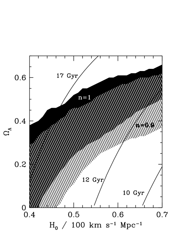
Figure 7: Acceptable values of $\Omega_{\Lambda}$ and $h$ for $n=0.9,1.0$. Note that large-scale structure considerations generally favor a more aged Universe – smaller $h$ or larger $\Omega_{\Lambda}$.

If CDM is correct, baryons make up a small fraction of matter in the Universe. Most of the baryons in galaxy clusters are in the hot, x-ray emitting intracluster gas and not the luminous galaxies. The measured x-ray flux fixes the mass in baryons, while the measured x-ray temperature fixes the total mass (through the virial theorem). The baryon-to-total-mass has been determined from x-ray measurements for more than ten clusters and is found to be $M_{\rm B}/M_{\rm TOT}\simeq(0.04-0.1)h^{-3/2}$.$\!{}^{{\bf?}}$ Because of their size, clusters should represent a fair sample of the cosmos and thus the baryon-to-total mass ratio should reflect its universal value, $\Omega_{B}/\Omega_{\rm Matter}\simeq(0.01-0.02)h^{-2}/\Omega_{\rm Matter}$. These two ratios are consistent for models with a very low Hubble constant, $h\sim 0.4$ and $\Omega_{\rm Matter}=1$, or with a cosmological constant and $\Omega_{\rm Matter}\sim 0.3$. However, important assumptions are made in this analysis – that the hot gas is unclumped and in virial equilibrium and that magnetic fields do not provide significant pressure support for the gas – if any one of them is not valid the actual baryon fraction would be smaller,$\!{}^{{\bf?}}$ allowing for consistency with a larger value of $H_{0}$ without recourse to a cosmological constant.

The halos of individual spiral galaxies like our own are not large enough to provide a fair sample of matter in the Universe – for example, much of the baryonic matter has undergone dissipation and condensed into the disk of the galaxy. Nonetheless, the content of halos is expected to be primarily CDM particles. This is consistent with the fact that visible stars, hot gas, dust, and even dark stars acting as microlenses (known as MACHOs) account for only a fraction of the mass of our own halo.$\!{}^{{\bf?},{\bf?}}$

Determining the mean mass density of the Universe would discriminate between models with and without a cosmological constant, as well as test the inflationary prediction of a flat Universe. A definitive determination is still lacking. The measurement that averages over the largest volume – and thus is potentially most useful – uses the peculiar velocities of galaxies. Peculiar velocities arise due to the inhomogeneous distribution of matter, and the mean matter density can be determined by relating the peculiar velocities to the observed distribution of galaxies. The results of this technique indicate that $\Omega_{\rm Matter}$ is at least 0.3 and perhaps as large as unity.$\!{}^{{\bf?},{\bf?}}$ Though not definitive, this provides strong evidence for the existence of nonbaryonic dark matter (see Fig. 4), a key aspect of cold dark matter.

A different approach to the mean density is through the deceleration parameter $q_{0}$, which quantifies the slowing of the expansion due to the gravitational attraction of matter in the Universe. Its value is given by $q_{0}={1\over 2}\Omega_{\rm Matter}-\Omega_{\Lambda}$ (vacuum energy actually leads to accelerated expansion) and can be determined by relating the distances and redshifts of distant objects. In all but the $\Lambda$CDM scenario, $q_{0}=0.5$; for $\Lambda$CDM, $q_{0}\sim-0.5$. Two groups are trying to measure $q_{0}$ by using high redshift ($z\sim 0.4-0.7$) Type Ia supernovae as standard candles; the preliminary results of one group suggest that $q_{0}$ is positive.$\!{}^{{\bf?}}$ More than a dozen distant Type Ia supernovae were discovered this year and both groups should soon have enough to measure $q_{0}$ with a precision of $\pm 0.2$.

Gravitational lensing of distant QSOs by intervening galaxies is another way to measure $q_{0}$, and the frequency of QSO lensing suggests that $q_{0}>-0.6$.$\!{}^{{\bf?}}$ The distance to a QSO of given redshift is larger for smaller $q_{0}$, and thus the probability for its being lensed by an intervening galaxy is greater.

The 10 m Keck Telescope and the Hubble Space Telescope are providing the deepest images of the Universe ever and are revealing details of galaxy formation as well as the formation and evolution of clusters of galaxies. The Keck has made the first detection of deuterium in high redshift hydrogen clouds.$\!{}^{{\bf?}}$ This is a new confirmation of big-bang nucleosynthesis and has the potential of pinning down the density of ordinary matter to a precision of 10%.

The level of inhomogeneity in the Universe today is determined largely from redshift surveys, the largest of which contain of order $10^{4}$ galaxies. A larger – a million galaxy redshifts – and more homogeneous survey, the Sloan Digital Sky Survey, is in progress.$\!{}^{{\bf?}}$ It will allow the power spectrum to be measured more precisely and out to large enough scales ($500h^{-1}\,{\rm Mpc}$) to connect with measurements from CBR anisotropy on angular scales of up to five degrees.

The most fundamental element of cold dark matter – the existence of the CDM particles themselves – is being tested. While the interaction of CDM particles with ordinary matter occurs through very feeble forces and makes their existence difficult to test, experiments with sufficient sensitivity to detect the CDM particles that hold our own galaxy together if they are in the form of axions of mass $10^{-6}{\,\rm eV}-10^{-4}{\,\rm eV}$$\!{}^{{\bf?}}$ or neutralinos of mass tens of GeV$\!{}^{{\bf?}}$ are now underway. Evidence for the existence of the neutralino could also come from particle accelerators searching for other supersymmetric particles. In addition, several experiments sensitive to neutrino masses are operating or are planned, ranging from accelerator-based neutrino oscillation experiments to the detection of solar neutrinos to the study of the tau neutrino at $e^{+}e^{-}$ colliders.

CBR anisotropy probes the power spectrum most cleanly as it is related directly to the distribution of matter when density perturbations were very small.$\!{}^{{\bf?}}$ Current measurements are beginning to test CDM and differentiate between the variants (see Fig. 2); e.g., a spectral index $n<0.7$ is strongly disfavored. More than ten groups are making measurements with instruments in space, on balloons and at the South Pole. Proposals have been made – three to NASA and one to ESA – for a satellite-borne experiment in the year 2000 that would map CBR anisotropy over the full sky with $0.2^{\circ}$ resolution, about 30 times better than COBE. The results from such a map could easily discriminate between the different variants of CDM (see Fig. 8).

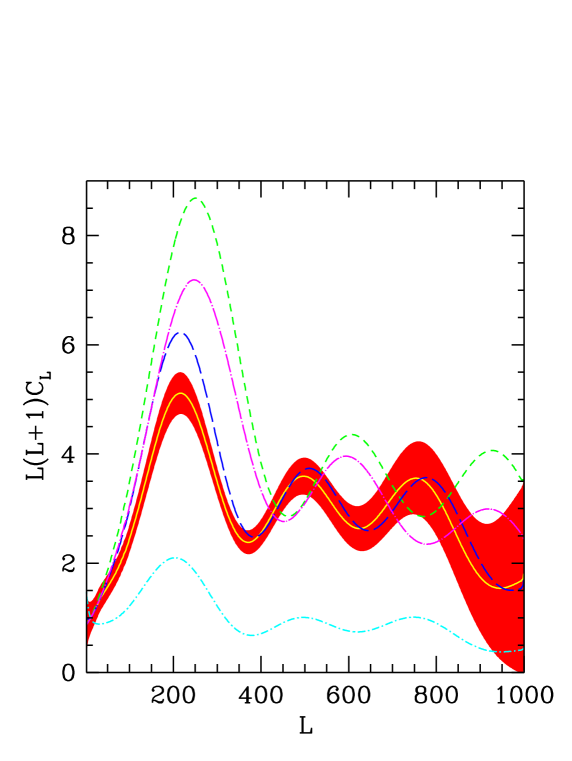
Figure 8: Predicted angular power spectra of CBR anisotropy for several viable CDM models (again in units of $7\times 10^{-10}$) and the anticipated uncertainty from a CBR satellite experiment with angular resolution of $0.3^{\circ}$. From top to bottom the models are: CDM with $h=0.35$, $\tau$CDM with the energy equivalent of 12 massless neutrino species, $\Lambda$CDM with $h=0.65$ and $\Omega_{\Lambda}=0.6$, $\nu$CDM with $\Omega_{\nu}=0.2$, and CDM with $n=0.7$ (unspecified parameters have their standard CDM values).

The first and most powerful test to emerge from these measurements will be the location of the first (Doppler) peak in the angular power spectrum (see Fig. 8).$\!{}^{{\bf?}}$ All variants of CDM predict the location of the first peak to lie in roughly the same place. On the other hand, in an open Universe (total energy density less than critical) the first peak occurs at a larger value of $l$ (much smaller angular scale). This will provide an important test of inflation. In addition, theoretical studies$\!{}^{{\bf?}}$ indicate that $n$ could be determined to a precision of a few percent, $\Omega_{\Lambda}$ to ten percent, and perhaps even $\Omega_{\nu}$ to enough precision to test $\nu$CDM.$\!{}^{{\bf?}}$

If all the current observations – from recent Hubble constant determinations to the cluster baryon fraction – are taken at face value, the cosmological constant + cold dark matter model is probably the best fit,$\!{}^{{\bf?}}$ though there may soon be a conflict with the measurement of $q_{0}$ with Type Ia supernovae. It raises a fundamental question – the origin of the implied vacuum energy, about $(10^{-2}{\,\rm eV})^{4}$ – since there is no known principle or mechanism that explains why it is less than $(300\,{\rm GeV})^{4}$, let alone $(10^{-2}{\,\rm eV})^{4}$.$\!{}^{{\bf?}}$ One possibility is that the Universe is in the midst of a mildly inflationary phase transition, in which case the nonzero vacuum-energy density is temporary.$\!{}^{{\bf?}}$

It would be imprudent to take all the observational data at face value because of important systematic and interpretational uncertainties. To paraphrase the biologist Francis Crick, a theory that fits all the data at any given time is probably wrong as some of the data are probably not correct.

5.3 Reconstruction

If inflation and the cold dark matter theory are shown to be correct, a window to the very early Universe ($t\sim 10^{-32}\,{\rm sec}$) will have been opened. While it is certainly premature to jump to this conclusion, I would like to illustrate one example of what one could hope to learn. The spectra and amplitudes of the the tensor and scalar metric perturbations predicted by inflation depend upon the underlying model, to be specific, the shape of the inflationary scalar-field potential. If one can measure the power-law index of the scalar spectrum and the amplitudes of the scalar and tensor spectra, one can recover the value of the potential and its first two derivatives around the point on the potential where inflation took place:$\!{}^{{\bf?}}$

$$V = 1.65T\,{m_{\rm Pl}}^{4},$$ (1)

$$V^{\prime} = \pm\sqrt{8\pi r\over 7}\,V/{m_{\rm Pl}},$$ (2)

$$V^{\prime\prime} = 4\pi\left[(n-1)+{3\over 7}r\right]\,V/{m_{\rm Pl}}^{2},$$ (3)

where $r\equiv T/S$ ($T$ is the contribution of tensor perturbations to the variance of the CBR quadrupole and $S$ is the same for scalar perturbations), prime indicates derivative with respect to $\phi$, ${m_{\rm Pl}}=1.22\times 10^{19}\,{\rm GeV}$ is the Planck energy, and the sign of $V^{\prime}$ is indeterminate. In addition, if the tensor spectral index can be measured a consistency relation, $n_{T}=-r/7$, can be used to further test inflation. Reconstruction of the inflationary scalar potential would shed light on the underlying physics of inflation as well as physics at energies of the order of $10^{15}\,{\rm GeV}$.

6 Concluding Remarks

The decade of the 1980s produced many bold and interesting speculations about the earliest history of the Universe, many involving the physics of the vacuum. Inflation and its cold dark matter theory of structure formation were so attractive that experimenters and observers paid them the highest praise possible – they took them seriously!

The decade of the 1990s is producing a flood of data that are testing inflation and cold dark matter. The stakes for both cosmology and fundamental physics are high: inflation and cold dark matter represent a major extension of the big bang and our understanding of the Universe, which would certainly shed light on fundamental physics at energies beyond the reach of terrestrial accelerators.

If inflation is correct, then vacuum energy played an important dynamical role in the evolution of the Universe at least once, and possibly twice, since the best fit cold dark matter model is one with a cosmological constant. Cosmology may soon have much to say about the physics of nothing.

References

- [1] G. ’t Hooft, Nucl. Phys. B 79, 276 (1974).
- [2] A. Polyakov, JETP Lett. 20, 194 (1974).
- [3] See e.g., A. Vilenkin, Phys. Rep. 121, 263 (1985); J. Preskill, Ann. Rev. Nucl. Part. Sci. 34, 461 (1984); E.J. Weinberg, ibid 42, 177 (1992).
- [4] N. Turok, Phys. Rev. Lett. 63, 2652 (1989); A. Gooding, D. Spergel, and N. Turok, Astrophys. J. 372, L5 (1991).
- [5] See e.g., T.D. Lee and Y. Pang, Phys. Rep. 221, 251 (1991).
- [6] D.A. Kirzhnits and A.D. Linde, Phys. Lett. B 42, 471 (1972).
- [7] A.H. Guth, Phys. Rev. D 23, 347 (1981).
- [8] See e.g., P.J.E. Peebles, D.N. Schramm, E. Turner, and R. Kron, Nature 352, 769 (1991); M.S. Turner, Science 262, 861 (1993).
- [9] See e.g., E.W. Kolb and M.S. Turner, The Early Universe (Addison-Wesley, Redwood City, CA, 1990).
- [10] A. Cohen, D. Kaplan, and A. Nelson, Annu. Rev. Nucl. Part. Sci. 43, 27 (1992).
- [11] See e.g., J. Huchra and M. Geller, Science 246, 897 (1989).
- [12] C. Copi, D.N. Schramm, and M.S. Turner, Science 267, 192 (1995).
- [13] M. White, D. Scott, and J. Silk, Science 268, 829 (1995).
- [14] A. Songaila et al., Nature 371, 43 (1994).
- [15] J.C. Mather et al., Astrophys. J. 420, 439 (1994); D.J. Fixsen et al., ibid, in press (1996).
- [16] A. Songaila et al., Nature 368, 599 (1994); R.F. Carswell et al., Mon. Not. R. astr. Soc. 268, L1 (1994); M. Rugers and C.J. Hogan, Astrophys. J. (Lett.), in press (1996) (astro-ph/9512004); D. Tytler, X.-M. Fan and S. Burles, astro-ph/9603069; S. Burles and D. Tytler, astro-ph/9603070; E.J. Wampler et al., Astron. Astrophys., in press (1996) (astro-ph/9512084); R.F. Carswell et al., Mon. Not. R. astron. Soc. 278, 506 (1996); M. Rugers and C.J. Hogan, astro-ph/9603084); L. Cowie and A. Songaila, in preparation (1996).
- [17] A. Reiss, R.P. Krishner, and W. Press, Astrophys. J. 438, L17 (1995); M. Hamuy et al, Astron. J. 109, 1 (1995); W. Freedman et al., Nature 371, 757 (1994).
- [18] M. Bolte and C.J. Hogan, Nature 376, 399 (1995).
- [19] C.B. Collins and S.W. Hawking, Astrophys. J. 180, 317 (1973).
- [20] Y. Hu, M.S. Turner, and E.J. Weinberg, Phys. Rev. D 49, 3830 (1994).
- [21] A. H. Guth and S.-Y. Pi, Phys. Rev. Lett. 49, 1110 (1982); S. W. Hawking, Phys. Lett. B 115, 295 (1982); A. A. Starobinskii, ibid 117, 175 (1982); J. M. Bardeen, P. J. Steinhardt, and M. S. Turner, Phys. Rev. D 28, 697 (1983).
- [22] V.A. Rubakov, M. Sazhin, and A. Veryaskin, Phys. Lett. B 115, 189 (1982); R. Fabbri and M. Pollock, ibid 125, 445 (1983); A.A. Starobinskii Sov. Astron. Lett. 9, 302 (1983); L. Abbott and M. Wise, Nucl. Phys. B 244, 541 (1984).
- [23] M.S. Turner and L.M. Widrow, Phys. Rev. Lett. 57, 2237 (1986); L. Jensen and J. Stein-Schabes, Phys. Rev. D 35, 1146 (1987); A.A. Starobinskii, JETP Lett. 37, 66 (1983).
- [24] A.D. Linde, Inflation and Quantum Cosmology (Academic Press, San Diego, CA, 1990).
- [25] A.D. Linde, Phys. Lett. B 108, 389 (1982).
- [26] A. Albrecht and P.J. Steinhardt, Phys. Rev. Lett. 48, 1220 (1982).
- [27] A.D. Linde, Phys. Lett. B 129, 177 (1983).
- [28] P.J. Steinhardt and M.S. Turner, Phys. Rev. D 29, 2162 (1984).
- [29] Q. Shafi and A. Vilenkin, Phys. Rev. Lett. 52, 691 (1984); S.-Y. Pi, ibid 52, 1725 (1984).
- [30] R. Holman, P. Ramond, and G.G. Ross, Phys. Lett. B 137, 343 (1984).
- [31] K. Olive, Phys. Repts. 190, 309 (1990).
- [32] H. Murayama et al., Phys. Rev. D(RC) 50, R2356 (1994).
- [33] L. Randall, M. Soljacic, and A.H. Guth, hep-ph/9601296.
- [34] M. Cvetic, T. Hubsch, J. Pati, and H. Stremnitzer, Phys. Rev. D 40, 1311 (1990).
- [35] E.J. Copeland et al., Phys. Rev. D 49, 6410 (1994).
- [36] See e.g., M. Gasperini and G. Veneziano, Phys. Rev. D 50, 2519 (1994); R. Brustein and G. Veneziano, Phys. Lett. B 329, 429 (1994); T. Banks et al., hep-th/9503114.
- [37] K. Freese, J.A. Frieman, and A. Olinto, Phys. Rev. Lett. 65, 3233 (1990).
- [38] L. Knox and M.S. Turner, Phys. Rev. Lett. 70, 371 (1993).
- [39] J. Silk and M.S. Turner, Phys. Rev. D 35, 419 (1986); L.A. Kofman, A.D. Linde, and J. Einsato, Nature 326, 48 (1987).
- [40] D. La and P.J. Steinhardt, Phys. Rev. Lett. 62, 376 (1991).
- [41] E.W. Kolb, Physica Scripta T36, 199 (1991).
- [42] M. Bucher A.S. Goldhaber, and N. Turok, Phys. Rev. D 52, 3314 (1995); M. Bucher and N. Turok, hep-ph/9503393.
- [43] M.S. Turner and F. Wilczek, Phys. Rev. Lett. 65, 3080 (1990); A. Kosowsky, M.S. Turner, and R. Watkins, ibid 69, 2026 (1992).
- [44] M.S. Turner and L.M. Widrow, Phys. Rev. D 37, 2743 (1988); B. Ratra, Astrophys. J. 391, L1 (1992).
- [45] L. Knox and M.S. Turner, Phys. Rev. Lett. 73, 3347 (1994).
- [46] M.S. Turner, J. Lidsey, and M. White, Phys. Rev. D 48, 4613 (1993).
- [47] See e.g., M.S. Turner, Physica Scripta T36, 167 (1991).
- [48] M. Fukugita, C.J. Hogan, and P.J.E. Peebles, Nature 366, 309 (1993); G. Jacoby et al, Proc. Astron. Soc. Pac. 104, 599 (1992).
- [49] S.D.M. White, C. Frenk and M. Davis, Astrophys. J. 274, L1 (1983).
- [50] A nice overview of the cold dark matter scenario is given by G. Blumenthal et al., Nature 311, 517 (1984).
- [51] See e.g., V. Trimble, Ann. Rev. Astron. Astrophys. 25, 425 (1987); M.S. Turner, Proc. Nat. Acad. Sci. (USA) 90, 4827 (1993).
- [52] See e.g., S. Parke, Phys. Rev. Lett. 74, 839 (1995); C. Athanassopoulos et al, ibid 75, 2650 (1995); J.E. Hill, ibid, 2654 (1995); K.S. Hirata et al, Phys. Lett. B 280, 146 (1992); Y. Fukuda et al, ibid 335, 237 (1994); R. Becker-Szendy et al, Phys. Rev. D 46, 3720 (1992).
- [53] H. Lin et al., Astrophys. J., in press (1996) (astro-ph/9602064).
- [54] G.F. Smoot et al., Astrophys. J. 396, L1 (1992).
- [55] J.P. Ostriker, Ann. Rev. Astron. Astrophys. 31, 689 (1993); A. Liddle and D. Lyth, Phys. Repts. 231, 1 (1993).
- [56] J. Peacock and S. Dodds, Mon. Not. R. astron. Soc. 267, 1020 (1994).
- [57] See e.g., P.J.E. Peebles and J.T. Yu, Astrophys. J. 162, 815 (1970); M.L. Wilson and J. Silk, Astrophys. J. 243, 14 (1981); J.R. Bond and G. Efstathiou, Astrophys. J. 285, L45 (1984); J. A. Holtzman, Astrophys. J. Suppl. 71, 1 (1989); A. van Dalen and R. K. Schaefer, Astrophys. J. 398, 33 (1992); N. Sugiyama and N. Gouda, Prog. Theor. Phys. 88, 803 (1992); S. Dodelson and J.M. Jubas, Phys. Rev. Lett. 70, 2224 (1993).
- [58] S. Dodelson, E.I. Gates, and M.S. Turner, astro-ph/9603081.
- [59] C.L. Bennett et al., Astrophys. J. (Lett.), in press (1996) (astro-ph/9601067); K.M. Gorski et al., Astrophys. J. (Lett.), in press (1996); M. White and E.F. Bunn, ibid 450, 477 (1995).
- [60] S.D.M. White, G. Efstathiou, and C.S. Frenk, Mon. Not. R. astron. Soc. 262, 1023 (1993).
- [61] K. Lanzetta, A.M. Wolfe, and D.A. Turnshek, Astrophys. J. 440, 435 (1995); L.J. Storrie-Lombardi, R.G. McMahon, M.J. Irwin, and C. Hazard, astro-ph/9503089.
- [62] C.-P. Ma and E. Bertschinger, Astrophys. J. 434, L5 (1994); A.R. Liddle et al., astro-ph/9511957.
- [63] M.S. Turner, G. Steigman, and L. Krauss, Phys. Rev. Lett. 52, 2090 (1984); M.S. Turner, Physica Scripta T36, 167 (1991); P.J.E. Peebles, Astrophys. J. 284, 439 (1984); G. Efstathiou et al., Nature 348, 705 (1990); L. Kofman and A.A. Starobinskii, Sov. Astron. Lett. 11, 271 (1985).
- [64] J. Bartlett et al., Science 267, 980 (1995).
- [65] R. Cen, N. Gnedin, L. Kofman, and J.P. Ostriker, ibid 399, L11 (1992); R. Davis et al., Phys. Rev. Lett. 69, 1856 (1992); F. Lucchin, S. Mattarese, and S. Mollerach, Astrophys. J. 401, L49 (1992); D. Salopek, Phys. Rev. Lett. 69, 3602 (1992); A. Liddle and D. Lyth, Phys. Lett. B 291, 391 (1992); J.E. Lidsey and P. Coles, Mon. Not. R. astron. Soc. 258, 57p (1992); T. Souradeep and V. Sahni, Mod. Phys. Lett. A 7, 3541 (1992); F. C.Adams, et al., Phys. Rev. D47, 426 (1993).
- [66] M. White, D. Scott, J. Silk, and M. Davis, Mon. Not. R. astron. Soc. 276, L69 (1995).
- [67] S. Dodelson, G. Gyuk, and M.S. Turner, Phys. Rev. Lett 72, 3578 (1994); J.R. Bond and G. Efstathiou, Phys. Lett. B 265, 245 (1991).
- [68] Q. Shafi and F. Stecker, Phys. Rev. Lett. 53, 1292 (1984); M. Davis, F. Summers, and D. Schlegel, Nature 359, 393 (1992); J. Primack et al., Phys. Rev. Lett. 74, 2160 (1995); D. Pogosyan and A.A. Starobinskii, astro-ph/9502019.
- [69] B. Chaboyer, P. Demarque, P.J. Kernan, and L.M. Krauss, Science bf 271, 957; M. Bolte and C.J. Hogan, Nature 376, 399 (1995).
- [70] J. Cowan, F. Thieleman, and J. Truran, Ann. Rev. Astron. Astrophys. 29, 447 (1991).
- [71] S.D.M. White et al., Nature 366, 429 (1993); U.G. Briel et al., Astron. Astrophys. 259, L31 (1992); D.A. White and A.C. Fabian, Mon. Not. R. astron. Soc. 273, 72 (1995).
- [72] A. Babul and N. Katz, Astrophys. J. 406, L51 (1993).
- [73] G.A. Luppino and N. Kaiser, astro-ph/9601194.
- [74] C. Alcock et al., Phys. Rev. Lett. 74, 2867 (1995); E. Gates, G. Gyuk, and M.S. Turner, ibid, 3724 (1995).
- [75] J. Bahcall et al., Astrophys. J. Lett. 435, L51 (1994); C. Flynn, A. Gould, and J. Bahcall, astro-ph/9603035.
- [76] M. Strauss and J. Willick, Phys. Repts. 261, 271 (1995).
- [77] A. Dekel, Ann. Rev. Astron. Astrophys. 32, 319 (1994).
- [78] S. Perlmutter et al., astro-ph/9602122.
- [79] See e.g., C.S. Kochanek, Astrophys. J., in press (1996) (astro-ph/9510077).
- [80] See e.g., J.E. Gunn and D.H. Weinberg, astro-ph 9412080 (1994).
- [81] L.J. Rosenberg, Particle World 4, 3 (1995).
- [82] D.O. Caldwell, in Particle and Nuclear Astrophysics in the Next Millennium, eds. E.W. Kolb and R.D. Peccei (World Scientific, Singapore, 1995), p. 38.
- [83] W. Hu and N. Sugiyama, Phys. Rev. D 51, 2599 (1995).
- [84] M. Kamionkowski, D.N. Spergel, and N. Sugiyama, Astrophysical J. 426, L57 (1994); G. Jungman, M. Kamionkowski, A. Kosowsky, and D. Spergel, Phys. Rev. Lett. 76, 1007 (1996); W. Hu and M. White, astro-ph/9602020.
- [85] L. Knox, Phys. Rev. D 52, 4307 (1995); G. Jungman, M. Kamionkowski, A. Kosowsky, and D. Spergel, Phys. Rev. D, in press (1996) (astro-ph/9512139).
- [86] S. Dodelson, E. Gates, and A.S. Stebbins, astro-ph/9509147 Astrophysical J., in press (1996).
- [87] L. Krauss and M.S. Turner, Gen. Rel. Grav. 27, 1137 (1995); J.P. Ostriker and P.J. Steinhardt, Nature 377, 600 (1995).
- [88] S. Weinberg, Rev. Mod. Phys. 61, 1 (1989).
- [89] C.T. Hill, J. Fry, and D.N. Schramm, Comments on Nuc. Part. Sci. 19, 25 (1991).
- [90] M.S. Turner, Phys. Rev. D 48, 3502 (1993); J. Lidsey et al., astro-ph/9508078.